High Mass Star Formation I: The Mass Distribution of Submillimeter Clumps in NGC 7538

Abstract

We present submillimeter continuum maps at 450 $\mu$m and 850 $\mu$m of a 12′$\times$8′ region of the NGC 7538 high-mass star-forming region, made using the Submillimeter Common-User Bolometer Array (SCUBA) on the James Clerk Maxwell Telescope. We used an automated clump-finding algorithm to identify 67 clumps in the 450 $\mu$m image and 77 in the 850 $\mu$m image. Contrary to previous studies, we find a positive correlation between high spectral index, $\alpha$, and high submillimeter flux, with the difference being accounted for by different treatments of the error beam. We interpret the higher spectral index at submillimeter peaks as a reflection of elevated dust temperature, particularly when there is an embedded infrared source, though it may also reflect changing dust properties. The clump mass-radius relationship is well-fit by a power law of the form M $\propto$ R^-x with $x$ = 1.5–2.1, consistent with theories of turbulently-supported clumps. According to our most reliable analysis, the high-mass end ($\sim$100–2700 M_⊙) of the submillimeter clump mass function in NGC 7538 follows a Salpeter-like power law with index $2.0\pm 0.3$. This result agrees well with similar studies of lower-mass regions $\rho$ Oph and Orion B. We interpret the apparent invariance of the shape of the clump mass function over a broad range of parent cloud masses as evidence for the self-similarity of the physical processes which determine it. This result is consistent with models which suggest that turbulent fragmentation, acting at early times, is sufficient to set the clump mass function.

1 Introduction

Although the form of the Galactic stellar initial mass function (IMF) has been accurately determined in the decades since Salpeter’s original paper on the subject, a definitive explanation of its origin is still lacking (Salpeter, 1955; Kroupa, 2002). Stars form from dense knots of dust and gas in the clumpy interstellar medium (ISM). Thus, to understand the origin of the stellar IMF, we must first understand the structure of the clumpy ISM and its origins. The relatively recent advent of sensitive submillimeter (submm) bolometer arrays has enabled us to begin studying the distribution of cold, dense, dusty molecular clumps in star-forming regions. Extensive studies of the submm clump distribution in low-mass star forming regions (e.g. Motte, André, & Neri 1998, Johnstone et al. 2000b, Motte et al. 2001) demonstrate that the mass function of pre-stellar clumps very closely resembles the Salpeter stellar IMF. This similarity implies that the stellar mass function is determined very early in the process of star formation, at least at low stellar masses. Turbulent fragmentation has been suggested as one process which might be able to account for the observed form of the clump mass function (Elmegreen & Falgarone, 1996; Elmegreen, 1997; Klessen, Burkert, & Bate, 1998; Padoan & Nordlund, 2002).

The structure of the cold, dusty ISM in regions of massive star formation remains relatively unexplored, though its study bears on several important problems in star formation. For example, it would be very helpful to know if the mass function of high-mass clumps is the same as that of low-mass clumps. Can turbulent fragmentation explain the origins of the clump mass function even at very high masses, or must some other mechanism, such as competitive accretion (Bonnell et al., 1997), be invoked? Because they contain clumps spanning several orders of magnitude in mass, massive star-forming regions bridge the gap between the scales on which individual stars form and the larger scales on which clusters form. Moreover, such studies have the potential to locate the cold, dense structures which may be the high-mass equivalents of the low-mass “Class 0” cores. Most previous studies of the structure of the dusty component of the ISM have concentrated on regions of low-mass, relatively non-turbulent star formation, such as $\rho$ Oph (Johnstone et al. 2000b, Motte, André, & Neri 1998). Comparatively little is known about the clump mass function in the turbulent, high-mass regime, partly due to observational challenges primarily arising from the large average distances of high-mass star-forming regions from the Sun. In this and a subsequent paper (Papers I and II), we use sensitive submm maps of two relatively nearby high-mass star-forming regions to measure the mass function of their cold, dusty clumps. In this paper, we present a 12′$\times$8′ (9$\times$6.5 pc) map of the Galactic star-forming region, NGC 7538, while Paper II presents a similar study of M17.

NGC 7538 is one of the nearest and youngest massive star-forming regions, whose proximity and relatively simple morphology make it an attractive candidate for this study. Located at a distance of 2.8 kpc (Crampton, Georgelin, & Georgelin 1978, but see also Moreno & Chavarria-K. 1986), NGC 7538 contains a prominent H II region centered on IRS 5 and surrounded by several highly active star-forming complexes. The brightest complex contains several very luminous infrared sources, IRS 1-3, each of which supports a young, compact H II region (Wynn-Williams, Becklin, & Neugebauer 1974, Rots et al. 1981). The IRS 9 and 11 regions show maser activity, while NGC 7538S, near IRS 11, contains a very young ($\lesssim 10^{4}$ yr) accreting “Class 0” high-mass protostar (Sandell, Wright, & Forster, 2003). All three of these complexes show significant CO outflow activity (Davis et al., 1998). NGC 7538 also contains several relatively quiescent, clumpy filaments trailing away from the more active centers, as seen in the NH₃ maps of Zheng et al. (2001). The apparent youth and relative proximity of NGC 7538 make it an excellent candidate for the study of the clump mass function in a high-mass star-forming region. Moreover, the quiescent regions at some distance from the H II region are promising locations for detecting the very cold, dense clumps which may represent the earliest stages of massive star formation.

Several other groups have mapped the large-scale structure of NGC 7538, in both spectral lines and continuum emission. Kramer et al. (1998) mapped an area of $\sim$21′$\times$24′ in ¹³CO (1$\rightarrow$0) and about half that area in C¹⁸O (1$\rightarrow$0); their data have a resolution of 50″ and are sensitive to the total column of gas, but have a smaller dynamic range than our continuum map. Zheng et al. (2001) used the VLA to map a slightly smaller region in NH₃ (1,1) and (2,2) with an 8″$\times$6″ beam. However, because the Zheng et al. (2001) map is interferometric, it is insensitive to structure on scales larger than $\sim 1$′. Sandell & Sievers (2004) mapped an 8′$\times$8′ region of NGC 7538 in 850 $\mu$m and 450 $\mu$m continuum with SCUBA. However, this early SCUBA map was made by chopping along the scan direction with a single chop throw, which can smear out structure along the scan direction. Also, the sensitivity of the map is relatively low (0.13 Jy beam^-1 at 850 $\mu$m and 0.9 Jy beam^-1 at 450 $\mu$m). The increased sensitivity and greater spatial coverage of our new SCUBA maps make them better suited to a study of the large-scale distribution of cold, dense clumps of NGC 7538.

Our analysis of the submillimeter clumps in the NGC 7538 region is divided into three sections. In section 2, we describe the acquisition, calibration, and reduction of the data. In section 3, we detail the methods used to determine the masses, temperatures, sizes, and other properties of the clumps. In section 4, we analyze and discuss the bulk properties of the clumps, including their mass-radius relationship and mass function. We summarize and conclude in section 5.

2 Observations and Data Reduction

The data were obtained on the nights of 2003 April 15, 16, 20, and June 16 using the Submillimeter Common-User Bolometer Array (SCUBA) at the James Clerk Maxwell Telescope (JCMT). The observed region is approximately 12′$\times$8′. The map was made with SCUBA in scan-mapping mode, using the standard chop throws of 30″, 44″, and 68″ in both RA and DEC. The total on-source integration time was approximately 7.5 hours. Pointing checks were performed once per hour and sky dips once every hour or two. The pointing accuracy varied from night to night, between 1.5″ and 3″, but was typically about 2″. The 850 $\mu$m and 450 $\mu$m sky opacities were calculated using polynomial fits to the combination of the JCMT skydips and the 225 GHz zenith optical depth measurements from the Caltech Submillimeter Observatory (CSO). The atmosphere was stable and fairly dry on all four nights, with mean 225 GHz zenith optical depths of 0.068, 0.063, 0.065, and 0.066, respectively. The mean residuals in the polynomial fits to the CSO optical depth translate into a systematic uncertainty in the fluxes of less than 1%.

The data were reduced using SURF, the standard SCUBA data reduction software (Jenness & Lightfoot, 1998). Map reconstruction from the six chop throws was done using the “Emerson2” method (Emerson, 1995; Jenness et al., 2000), with pixels 2″ on a side. The mean rms flux measured in emission-free regions of the maps is 0.021 Jy beam^-1 at 850 $\mu$m and 0.18 Jy beam^-1 at 450 $\mu$m. The half-power beam widths at 850 $\mu$m and 450 $\mu$m were measured to be 15.3″ and 8.1″, respectively. The maps were calibrated using both primary (Uranus and Mars) and secondary (CRL2688) calibrators. Making the conservative assumption that the night-to-night variations in the gains calibration are entirely due to measurement error, we determine the uncertainty due to the gains to be 12% at 450 $\mu$m and 4% at 850 $\mu$m.

As discussed by Johnstone et al. (2000a), reconstruction of a SCUBA scan map image from its component chop throws using the Emerson2 technique introduces artifacts that should be removed prior to further analysis. These artifacts take the form of spurious structure in the image on scales significantly larger than the largest chop throw (i.e. a few arcminutes, in the present case). Often, the presence of a very strong source, such as NGC 7538 IRS1, will introduce regions of negative flux (so-called “negative bowls”) in its vicinity. Because our chosen clump-finding algorithm, clfind2d (Williams, de Geus, & Blitz, 1994), functions best on images without such negative bowls, we have taken steps to suppress them. Johnstone et al. (2000b) showed that the simple addition of a constant flux to the map to eliminate bowls does not adequately address all of the sources of spurious long-wavelength structure in the image. We employ a method similar to that of Johnstone et al. (2000b) to suppress the bowls, namely convolving each map with a Gaussian twice the width of the largest chop throw and subtracting the result from the original image. Because the chop technique itself screens out all emission on scales much larger than the largest chop throw, this technique eliminates only the artificial long-wavelength modes. In order not to introduce new negative bowls in the image by smearing out and then subtracting bright sources, we masked out all pixels with $|S|>5\sigma$ before producing the smoothed image. This technique leaves the image rms unchanged and does not significantly change the height of a given peak with respect to its local surroundings, but it mostly removes the negative bowls. This greatly facilitates the process of clump-finding. Comparisons between matching clumps in the “flattened” and unflattened images shows a difference in their integrated fluxes of only a few percent, well below the level of the calibration uncertainties.

We used the 6 cm continuum map of Israel (1977) to correct our data for radio continuum emission. Using the Westerbork Synthesis Radio Telescope, Israel (1977) mapped the H II region and sources IRS1-3 in NGC7538 at 5 GHz. The synthesized beam of their map is $\sim 14$″, which nearly matches the 15″ resolution of our 850 $\mu$m map. We derived free-free corrections for each clump by comparing its peak fluxes at 850 $\mu$m and 6 cm and assuming a scaling law of $S_{\nu}\propto\nu^{-0.1}$ for the radio continuum emission. The worst contamination occurs in clump SMM34, which lies directly over the center of the optical H II region. We estimate the free-free contamination there to be $\sim 20$%. Similarly, we estimate the contamination of clump SMM48, which includes the compact H II regions of IRS 1-3, to be $\sim 8$%. Elsewhere, the free-free contamination is typically on the order of a few percent. Free-free corrections were found to be negligible at 450 $\mu$m.

Corrections for contamination of the 850 $\mu$m filter by CO(3$\rightarrow$2) line emission were derived according to the method of Seaquist et al. (2004). We used archival CO (3$\rightarrow$2) spectra of IRS 1 and IRS 9 to derive corrections to the 850 $\mu$m fluxes of $\sim 3$% and $\sim 10$%, respectively. The best available CO map of NGC 7538 is that of Davis et al. (1998), who used the JCMT to make a $\sim$ 7′$\times$5′ CO(2$\rightarrow$1) map of the central part of NGC 7538 (roughly 40% of the area of our map). Under the assumption that the CO(2$\rightarrow$1) traces the CO(3$\rightarrow$2) fairly closely, we derived corrections to the 850 $\mu$m fluxes for the clumps covered by the Davis et al. (1998) map. These are typically less than 15%, and are likely to be further reduced (by perhaps a factor of two or more) by the fact that our observations are chopped, whereas the CO(2$\rightarrow$1) map traces the total flux. Because these corrections are relatively small and only calculable for the roughly half of our clumps covered by the Davis et al. (1998) map, we have not applied any correction for CO contamination to the data.

A final correction must be made to account for the contribution of the error beam to the integrated flux of each clump, which is especially significant at 450 $\mu$m. The JCMT error beam can vary significantly on timescales as short as a few weeks, so we derived fits to the error beam at 850 $\mu$m and 450 $\mu$m using our own calibration observations of Uranus and CRL 2688. We produced azimuthally averaged intensity profiles for each calibrator and then fit them with two Gaussians each: a narrow Gaussian of high amplitude, corresponding to the primary beam, and a broad, low amplitude Gaussian, corresponding to the error beam. We attempted to fit a third, very low amplitude Gaussian, but were unsuccessful due to signal-to-noise limitations. Our estimates indicate that this third component contributes at most 4% of the flux within a 120″ aperture, and is therefore negligible. The results of our beam fits are shown in Table 1. The beam fits to Uranus and CRL 2688 agree within the errors and are very similar to those reported by Hogerheijde & Sandell (2000). Henceforth, we use the Uranus beam fits, which have smaller uncertainties. We correct the integrated flux of each clump for the contribution of the error beam within an aperture of radius equal to the clump’s effective radius. A clump’s effective radius is defined as the radius of a circle of equal area to the clump. The maximum error beam correction applied at 850 $\mu$m was 14%, and the typical correction was between 3 and 10%. Similarly, the largest correction applied at 450 $\mu$m was 19% and the typical value was between 5 and 15%. The uncertainty in the error beam correction itself was taken to be half the difference between the corrections due to the maximal and minimal error beams, which are defined by the uncertainty ranges in Table 1.

3 Properties of the NGC 7538 Clumps

3.1 The Filamentary Global Morphology of NGC 7538

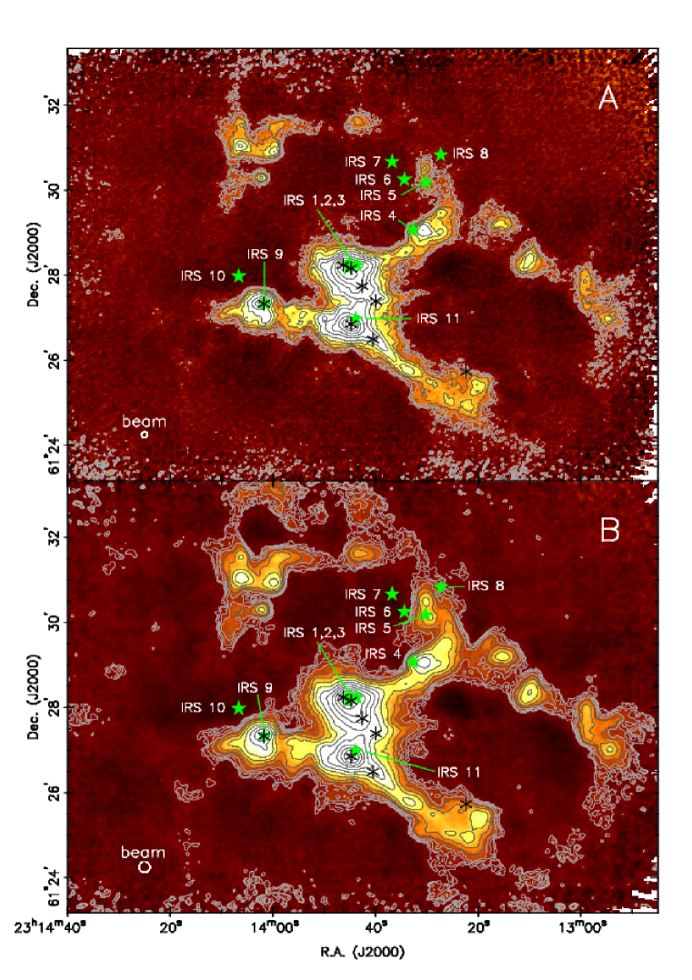
Figure 1: Submillimeter continuum images of NGC 7538 at 450 $\mu$m (A) and 850 $\mu$m (B), in greyscale with logarithmically spaced contours. The 450 $\mu$m contours begin at 3$\sigma$ (0.54 Jy beam^-1) and the 850 $\mu$m contours begin at 3$\sigma$ (0.063 Jy beam^-1); both increase by factors of 1.5. Stars represent the positions of IRS point sources (Wynn-Williams, Becklin, & Neugebauer 1974,Werner et al. 1979). Asterisks represent the positions of water masers from Kameya et al. (1990). For visual clarity, only a representative sample of the many masers in the IRS 1-3, 9, and 11 regions are shown.

NGC 7538 is an excellent example of a filamentary star-forming region, as can be seen in the maps of Sandell & Sievers (2004) and, to a larger extent, in Figure 1. Most of the larger clumps are located along filaments, although several smaller and apparently smooth filaments are also visible. The clumps associated with IRS 9 and 11 are connected in a single long filament which stretches several parsecs southwest of IRS 11. Another filament connects IRS 1-3, IRS 4, and IRS 5, then continues southwest of IRS 5. These two filaments may be joined in a bubble-like structure by a faint bridge in the southwest corner of the image.

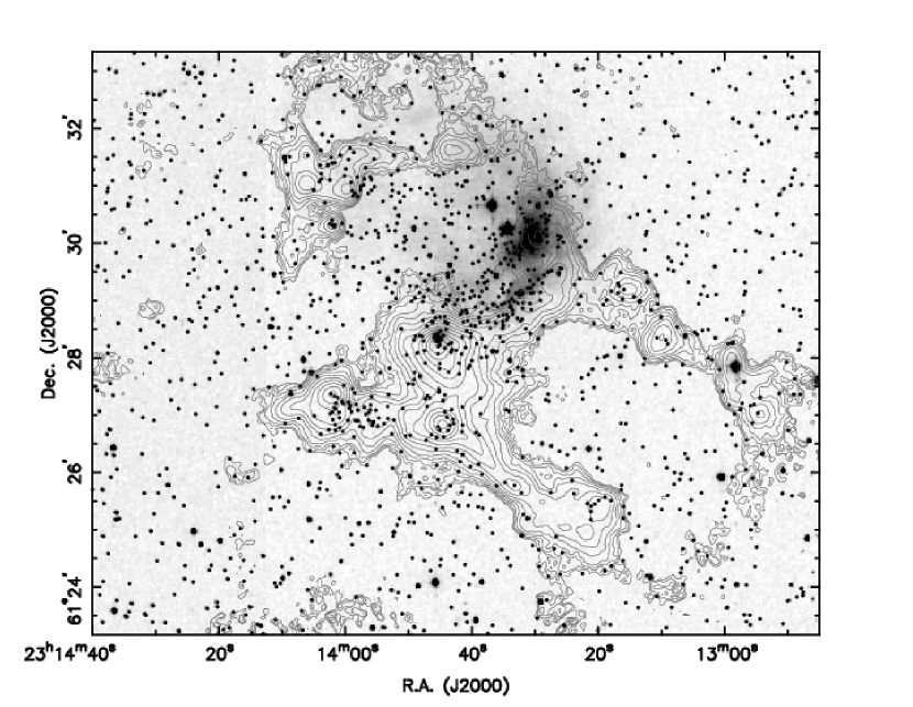
Figure 4: Comparison of 850 $\mu$m submm emission (contours, as in Fig. 1) with 2MASS J image (greyscale) and 2MASS point sources (black dots). The H II region is the diffuse feature filling the submm void to the north of the prominent IRS 1-3 group. Note the significant over-density of infrared point sources in the IRS 1-3, 9, and 11 regions. Of the 850 $\mu$m clumps, 69% show coincidence of a point source within their 0.5$S_{\rm peak}$ contour.

We see strong evidence of interaction between the optical H II region in NGC 7538, which is centered on IRS 5 (see Figure 4), and the submm-emitting material. Although IRS 5 itself is coincident with a submillimeter clump, most of the extended faint emission from the H II region sits in a submm void. The steep gradient in the submm walls of this void suggests compression by a wind originating in the H II region, which may have triggered much of the present star formation activity in surrounding clumps.

3.2 Clump Identification Using clfind2d

In order that our method of identifying clumps be both systematic and reproducible, we chose to use the popular clfind2d program (Williams, de Geus, & Blitz, 1994). The clfind2d algorithm typically works by contouring a map at three times the image rms, $\sigma$, and at intervals of 2$\sigma$ above that. We found that, to improve the performance of the algorithm in this region with considerable clustered substructure, it was necessary to set the contour interval to $1\sigma$ when processing the 850 $\mu$m image. Had we not done so, many closely-spaced clumps would have been merged into “plateaus” by clfind2d. We reprocessed the output of clfind2d to merge clumps whose peaks were separated by less than $2\sigma$, recovering a similar (but not identical) result to that generated by the algorithm in its default mode of operation. For the 450 $\mu$m map, which has higher spatial resolution, we found it sufficient to contour at the recommended $2\sigma$ level. In this way, we identify very similar structures in both maps.

We emphasize that the choice of clump-finding algorithm introduces biases into the clump properties. For example, because clfind2d attempts to assign all of the flux in an image to clumps, the masses and radii of the some clumps are likely to be overestimated, particularly in highly clustered regions.

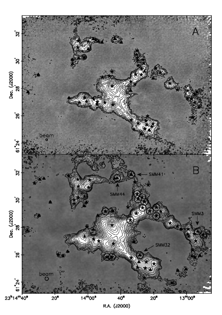
Figure 2: The positions of the detected clumps in NGC 7538 at 450 $\mu$m (A) and 850 $\mu$m (B). Contours are the same as in Figure 1. Symbols indicate the peak positions of identified clumps which do (stars) and do not (triangles) show coincidence with a 2MASS point source within their 0.5$S_{\rm peak}$ contour. Circled symbols in the 850 $\mu$m image indicate “cold” clumps (i.e. those with estimated dust temperatures, T${}_{\rm dust}\leq 30$ K). Thus, a circled triangle indicates a possible cold, starless clump; the four such clumps are labelled.

In all, 77 clumps were identified in the 850 $\mu$m image and 67 in the 450 $\mu$m image. These clumps and their derived properties are listed in Tables 2 and 3. The positions of the clump peaks are indicated in Figure 2. The differences in clump numbers and boundaries between the two images arise because of the higher signal-to-noise ratio (SNR) of the 850 $\mu$m image and the higher resolution of the 450 $\mu$m image. The angular resolution of the 450 $\mu$m image is nearly double that of the 850 $\mu$m image, so some of the 850 $\mu$m clumps resolve into two or more clumps in the 450 $\mu$m image. For example, the IRS 9 region, which appears as a single clump in the 850 $\mu$m image, is resolved into four separate clumps in the 450 $\mu$m image. The high SNR of the 850 $\mu$m image reveals several faint clumps not detected in the 450 $\mu$m image. It also helps to distinguish closely spaced clumps with similar peak fluxes, which may appear as a single elongated clump in the 450 $\mu$m image.

Comparison of the clump identifications from the 850 $\mu$m and 450 $\mu$m images reveals that 41 of the 850 $\mu$m clumps are spatially coincident with 450 $\mu$m clumps. Of these 41 clumps, only 16 resolve into more than one clump in the 450 $\mu$m image, which has nearly double the resolution. This comparison suggests that most of the clumps seen in the 850 $\mu$m image are coherent physical structures, rather than superpositions of unrelated smaller structures. Possible significant exceptions include the clumps surrounding IRS 1-3 (SMM48) and IRS 9 (SMM60). In both cases, the shapes of the contours near the clump peaks suggest partially-resolved substructure, but the flux differences among the sub-peaks are sufficiently small that the clfind2d algorithm groups them together. Sandell & Sievers (2004) used the CLEAN algorithm to improve the resolution of their continuum images of NGC 7538, achieving resolution of 7″ at 450 $\mu$m. Their maps show more substructure in the IRS 1-3 and IRS 9 regions, and may provide a clearer picture of the local source structure. We interpret their results cautiously, however, as their scan maps show evidence of spurious elongation of structures along the scan direction.

3.3 Clump Masses

If the dust emission is optically thin, the total mass of a clump can be calculated from

$${\rm M}_{\rm clump}=\frac{S^{\rm int}_{\lambda}d^{2}}{\kappa_{\lambda}B_{\lambda}({\rm T}_{\rm dust})}~{}~{},$$ (1)

where ${\rm M}_{\rm clump}$ is the mass of the clump, $S^{\rm int}_{\lambda}$ is the flux of the clump at wavelength $\lambda$ integrated over the boundary defined by clfind2d, $d$ is the distance to the clump, $\kappa_{\lambda}$ is the dust opacity per unit mass column density at wavelength $\lambda$, and $B_{\lambda}({\rm T}_{\rm dust})$ is the Planck function at wavelength $\lambda$ and dust temperature T_dust.

Because determining both the temperature and the dust opacity for each clump individually is usually not possible, a number of simplifying assumptions must be made. The simplest strategy is to assume that each clump can be represented by a single volume-averaged dust opacity and dust temperature, and that these values do not vary from clump to clump (e.g. Johnstone et al. 2000b). Another common strategy is to break clumps into categories and to assign a volume-averaged dust opacity and temperature to all of the clumps in each category (c.f. Motte, André, & Neri 1998, Johnstone et al. 2000b, Motte, Schilke, & Lis 2003). For this study, we assume that all clumps are represented by the same volume-averaged dust opacity. By fitting spectral energy distributions, Sandell & Sievers (2004) determined values of the dust emissivity index, $\beta$, of 1.2, 1.6, and 2 for the IRS 1, 11, and 9 clumps, respectively, although these values are considerably uncertain. For simplicity, we will assume $\beta=1.5$ for all clumps. Hence, assuming a gas-to-dust ratio of 100 and taking the prescription from Hildebrand (1983) that $\kappa_{\lambda}=0.1(250\mu\mbox{m}/\lambda)^{\beta}$ cm² g^-1, we obtain $\kappa_{850\mu{\rm m}}=0.0087$ cm² g^-1 and $\kappa_{450}=0.031$ cm² g^-1. This is the same prescription for the dust opacity used by Sandell & Sievers (2004). Our values are also similar to the dust opacities used by Motte et al. (2001), who used $\kappa_{850\mu{\rm m}}=0.01$ cm² g^-1 for starless clumps and $\kappa_{850\mu{\rm m}}=0.02$ cm² g^-1 for protostellar envelopes in Orion, and by Johnstone et al. (2000b), who used $\kappa_{850\mu{\rm m}}=0.01$ cm² g^-1 for all of their detected clumps in $\rho$ Oph.

The remaining free parameter in Equation 1 is the dust temperature. Again, the simplest approach is to assume that all clumps are isothermal and share the same temperature. In crowded massive star-forming regions, where each clump may contain one or more strong central heating sources, the assumptions of an isothermal equation of state and an invariant temperature are certainly approximate. Nonetheless, lacking suitable data for a more detailed analysis (and for ease of comparison with previous work), we adopt this approach. By performing SED fits, Sandell & Sievers (2004) found dust temperatures for the IRS 9 and IRS 11 regions of 35 K. To facilitate comparison of our results with theirs, we adopt 35 K as our universal dust temperature. The masses thus calculated are given in Tables 2 (850 $\mu$m clumps) and 3 (450 $\mu$m clumps). The 850 $\mu$m masses range from 1.4 to 2700 M_⊙ and the 450 $\mu$m masses range from 4 to 3000 M_⊙, straddling the regimes of stellar-mass objects and cluster-mass objects.

Our integrated fluxes and masses are considerably higher than those of Sandell & Sievers (2004). This likely due to a combination of the higher sensitivity of our maps and to differences between the two studies in the boundary definitions of highly clustered clumps. Because clfind2d attempts to assign all of the flux in a map to clumps, the higher sensitivity of our maps means that our integrated fluxes include more of the extended emission from each clump. In cases where there is a one-to-one correspondence between the 850 $\mu$m and 450 $\mu$m clumps and good agreement between the clfind2d-determined boundaries, the mean difference between the two mass estimates is 12%. For example, the masses we derive for the NGC 7538S/IRS11 clump (SMM46 and SMM46A, by our notation) are $2200\pm 300$ M_⊙ at 850 $\mu$m and $2300\pm 400$ M_⊙ at 450 $\mu$m. Similarly, for clumps SMM63 and SMM57 (the two adjoining bright clumps in the northeast corner of the image), we derive 850 $\mu$m masses of $140\pm 20$ M_⊙ and $110\pm 10$ M_⊙ respectively, compared to 450 $\mu$m masses of $140\pm 20$ M_⊙ and $100\pm 20$ M_⊙. Where the agreement between the clump boundaries is poor, the mean difference in masses rises to 33%.

3.4 Dust Properties: Spectral Index and Temperature

By dividing one of our maps by the other, we can produce a map of the spectral index variations within NGC 7538. The spectral index, $\alpha$, takes the form,

$$\alpha=\frac{\log(S_{450\mu{\rm m}}/S_{850\mu{\rm m}})}{\log(850/450)}~{}~{}.$$ (2)

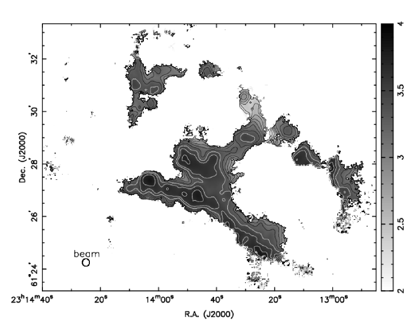
Figure 3: Map of the spectral index in NGC 7538, produced by convolving the 850 $\mu$m and 450 $\mu$m images with each others’ beams and dividing the two images. The effective beam size of the map is $\sim$17″. The contours are linearly spaced at intervals of $\alpha=0.15$; the lowest white contour is $\alpha=3.4$. Only pixels in which emission was detected at $>3\sigma$ in both filters are represented in the ratio map.

Before dividing one image by another, we must ensure that they have not only a common resolution, but a common beam structure. Because the error beams at 850 $\mu$m and 450 $\mu$m differ so much (see Table 1), it is not sufficient to simply match the main beam structure by convolving the 450 $\mu$m image to the same resolution as the 850 $\mu$m image. To produce 850 $\mu$m and 450 $\mu$m images with fully matched beams, we convolved each of the “flattened” images with the beam at the opposing wavelength. We then divided the convolved images and masked out all pixels which were not detected at $\geq 3\sigma$ in both original images. The result is a “ratio map” with spatial resolution of $\sim$ 17″(slightly coarser than the 850 $\mu$m image). The cross-convolutions alter the flux scaling in each map, so we must re-calibrate the ratio map. To derive the appropriate calibration factor, we applied the same set of convolutions to the Uranus images and compared the derived flux ratio with the one expected from tabulated fluxes for Uranus at the time of our observations. This gave a correction factor of 2.18, which we applied to the $S_{450\mu{\rm m}}/S_{850\mu{\rm m}}$ map. The flux ratio map was converted to a spectral index map using Equation 2; the result is shown in Figure 3.

We find a fairly consistent correlation between high submillimeter flux and high spectral index, particularly in the bright regions around IRS 1-3, 9, and 11. Notable exceptions to this trend include the large group of clumps in the southwest corner of Fig. 3 and the group at the western edge of the image. In both cases, there is a fairly smooth gradient in $\alpha$ which does not reflect the locally peaky nature of the submillimeter continuum emission (cf. Fig. 1). Both regions border the bubble-like structure which dominates the western half of the region.

Note that this correlation between high $\alpha$ and high continuum flux is the opposite trend to that found by Font, Mitchell, & Sandell (2001) in their SCUBA study of star-forming region NGC 7129. We believe the discrepancy can be explained by the different methods used to account for the error beam. Font, Mitchell, & Sandell (2001) account for the error beam by adding a constant level of 5% of the peak flux to the 450 $\mu$m map before convolving it to the same resolution as their 850 $\mu$m map and dividing. If we follow the same procedure with our data, we also find a consistent anti-correlation between submillimeter continuum flux and spectral index. However, this technique for constructing an $\alpha$ map does not account for the spatially-varying contribution of the 450 $\mu$m error beam, and hence results in comparison between images with mis-matched beams.

For a given pair of frequencies, the spectral index, $\alpha$, depends on the dust emissivity, $\beta$, and a temperature-dependent correction to the Rayleigh-Jeans form of the Planck function (see Eqs. 5 and 6 of Font, Mitchell, & Sandell 2001). An increase in $\alpha$ may arise due to an increase in either or both of T and $\beta$. For those clumps known to have embedded infrared point sources, such as IRS 1-3, 9, and 11, the observed increase in $\alpha$ toward the submillimeter peak may plausibly be ascribed to an increase in the dust temperature. Larger-scale gradients, such as those described above, may also reflect temperature gradients. Alternatively, they could be the result of changing dust properties (the formation of larger or smaller grains, for example).

In section 3.3, we assumed a spatially invariant dust emissivity index $\beta=1.5$. If we again make this simplifying assumption, we can use the ratio map to calculate the temperature of any submillimeter-emitting parcel of dust via (Mitchell et al., 2001):

$$\frac{S_{450_{\mu{\rm m}}}}{S_{850_{\mu{\rm m}}}}=\frac{e^{16.9/T}-1}{e^{32.0/T}-1}\left(\frac{850}{450}\right)^{3+\beta}~{}~{}.$$ (3)

For those 850 $\mu$m clumps with five or more pixels in the ratio map, we used Equation 3 to convert the mean flux ratio in these pixels to a mean dust temperature for the clump. (Due to the significant resolution mismatch between the 450 $\mu$m map and the ratio map, this technique is not applicable to the 450 $\mu$m clumps.) Equation 3 asymptotes to a maximum flux ratio for a given $\beta$ (approximately 9.3 for $\beta=1.5$). No temperatures were calculated for clumps with mean flux ratios above this value (the existence of such high flux ratios is likely a reflection of a spatially varying $\beta$). Subject to these constraints, we are able to estimate mean temperatures for 42 of the 77 original 850 $\mu$m clumps. These temperatures appear in Table 2. The range of estimated temperatures is 8–329 K, with a median of 35 K. Typical uncertainties on these temperatures, derived from the systematic errors in the gains, sky opacities, and error beam fits, are $\pm$5 K for T $\lesssim~{}20$ K and ${}^{+20}_{-10}$ K for 20 K$<$T$<$ 50 K. Above 50 K, all we can say with confidence is that the clump is hotter than $\sim$30 K. In this sense, our temperature estimates can be interpreted as lower limits on the real temperature of each clump. Clump masses derived using these estimated temperatures and Eq. 1 are also given in Table 2.

3.5 Evolutionary States: Correlations with Signposts of Massive Star Formation

The NGC 7538 region is known to contain several objects in the earliest stages of massive star formation. Sandell, Wright, & Forster (2003) give strong evidence from both continuum and line observations for the presence of a candidate “Class 0” massive protostar in the NGC 7538S region (near IRS 11). The object contains a Keplerian disk approximately 30,000 AU in extent with mass $\gtrsim 100$M_⊙, surrounding a central object of mass $\sim 40$M_⊙. This object powers a strong outflow whose dynamical age is estimated to be less than 10⁴ yr. Similarly, CS (2$\rightarrow$1) observations by Davis et al. (1998) reveal powerful outflows emanating from the IRS 1 and 9 regions, with dynamical ages of 1.5$\times 10^{4}$ yr and 4.2$\times 10^{4}$ yr, respectively. This evidence strongly suggests that NGC 7538 is a site of vigorous, ongoing massive star formation and motivates us to probe the evolutionary states of its cold, dusty clumps.

Maser surveys offer one tool for locating potential sites of massive star formation. In Figure 1, we have plotted the positions of 22 GHz H₂O masers detected by Kameya et al. (1990) in their survey of the central 8′$\times$8′ of NGC 7538. These H₂O masers trace all of the known sites of maser emission in NGC 7538 (including those in other transitions, such as methanol and OH), most of which are concentrated in the IRS 1-3, 9, and 11 regions. The notable exception is the maser which lies roughly 3′ southwest of IRS 11, which is the brightest H₂O maser in the region. It lies within the 850 $\mu$m clump SMM26 and the 450 $\mu$m clump SMM26B, though not at the peak of either. It may represent the location of an as-yet unidentified massive protostar. All of the other known sites of maser emission fall within the boundaries of the submillimeter clumps associated with IRS 1-3, 9, and 11.

We used the 2MASS maps of NGC 7538 (Fig. 4) to search for embedded infrared point sources, whose presence in a given clump would indicate past or ongoing star formation. Unfortunately, the absence of such point sources cannot be taken as counter-evidence of star formation; recent results from Spitzer show that, even for low-mass cores, some “starless” cores actually contain heavily-extincted infrared sources (Young et al., 2004). The highest-resolution infrared data available for the entire NGC 7538 region come from 2MASS (see Fig. 4). The 2MASS exposures are deep enough to locate some of the embedded sources, but are insufficiently deep to rule out definitively the presence of an embedded infrared source in any particular clump. In Tables 2 and 3, we specify the number of 2MASS point sources which lie within the 0.5S_peak contour of each clump. Associations between submillimeter clumps and IRS sources (Wynn-Williams, Becklin, & Neugebauer, 1974) are listed in Table 4. Overall, 69% of the 850 $\mu$m clumps contain one or more such point sources, compared to 32% of the 450 $\mu$m clumps; however, this result does not necessarily mean that 69% of the clumps have embedded protostars. The density of 2MASS point sources within the local field is about 60% of the density of such sources within the $>3\sigma$ submillimeter-emitting region, so many of the point sources coincident with submm clumps are certainly field stars. The exact fraction of “starless” clumps in our dataset is impossible to determine with the data at hand but, based on the above analysis, we estimate it to be around 50%.

We expect that the very youngest pre-stellar clumps will be those which are cold and which do not possess an embedded infrared point source. Examination of Table 2 reveals several objects which are cold (mean T$\leq 30$K) and contain no 2MASS point source within their 0.5$S_{\rm peak}$ contour (clumps SMM3, 32, 41, and 44). These would be logical candidates for infrared and high-resolution spectral line and continuum follow-up. There may be other cold, potentially starless clumps within the sample for which we were not able to calculate a temperature.

4 Clump Mass Distributions: Evidence for Turbulent Fragmentation

4.1 Clump Mass-Radius Relation

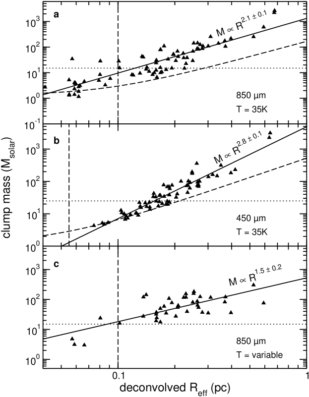
Figure 5: Mass vs. deconvolved radius for three ensembles of clumps, with masses calculated using the temperatures as indicated. Panels (a), (b), and (c) include 77, 67, and 42 clumps, respectively. Horizontal dashed lines indicate the estimated completeness thresholds of 15 M_⊙ at 850 $\mu$m and 25 M_⊙ at 450 $\mu$m. The curving dashed lines in panels (a) and (b) indicate the mass detection threshold as a function of deconvolved radius. Vertical dashed lines represent the beam radius; clumps to the left of this line are unresolved. Mass error bars are omitted for clarity, but are typically close to the size of the plotted points. The solid lines are least-squares fits to power laws of the form ${\rm M}\propto R^{x}$.

Assessing the completeness of a sample of clumps extracted from a submillimeter map is complicated by the fact that the clumps are not point sources. Hence, the detection limit is not an absolute cutoff in flux, but rather a limiting rms surface brightness. For example, a spatially-extended high-mass clump, even with a large integrated flux, can be more difficult to detect than a compact, low-mass object. Therefore, the mass detection threshold must be expressed as function of the effective clump radius. Figure 5 shows the mass-radius relation for the 850 $\mu$m and 450 $\mu$m clumps with constant-temperature masses, illustrating the dependence of the detection threshold on clump size. We define our smallest detectable clump as one with an area equal to at least half that of the beam, whose flux is everywhere $\geq 3\sigma$ and whose peak flux is $\geq 5\sigma$. As seen in Fig. 5, it is difficult to specify the mass above which the clump sample is complete. We estimate a lower completeness threshold of 15 M_⊙ at 850 $\mu$m and 25 M_⊙ at 450 $\mu$m, although we emphasize the considerable uncertainty in these estimates.

Least-squares fits of the mass-radius data to a power law of the form ${\rm M}\propto{\rm R}^{x}$ are shown in Figure 5. The 850 $\mu$m and 450 $\mu$m constant-temperature mass-radius relations are best fit by $x=2.1\pm 0.1$ and $2.8\pm 0.1$, respectively. A fit to the 42 clumps whose masses were calculated using the temperatures estimated from the ratio map gives $x=1.5\pm 0.2$ (Fig. 5c). None of the fits change substantially if we exclude the clumps below the estimated completeness threshold.

Previous studies of the mass-radius relationship of submillimeter clumps have concentrated on regions dominated by low-mass clumps, such as NGC2068/2071 and $\rho$ Oph. They have typically found $x\simeq 1$ (Motte et al., 2001). This is the expected result for an ensemble of thermally-supported Bonnor-Ebert spheres (Bonnor, 1956; Ebert, 1955). Similar studies of the mass-radius relationship of CO clumps, spanning the mass range $\sim 10^{-2}-10^{3}$ M_⊙ have typically found $x\simeq 2$ (Larson 1981, Elmegreen & Falgarone 1996). Note, however, that this result only emerges when the CO clumps from many regions are analyzed as an ensemble (Elmegreen & Falgarone, 1996); the power laws measured in each individual region have $x=2.3-3.7$, with values $>3$ being typical. A value of $x=2$ is consistent with the theoretical picture in which a turbulent molecular cloud fragments, producing a fractal distribution of clump masses and sizes (Elmegreen & Falgarone 1996, Elmegreen 1997). It is also the result predicted for an ensemble of turbulently supported clumps, such as the logotropic spheres of McLaughlin & Pudritz (1996).

We cannot rule out the possibility that the steep power law fit to the mass-radius relation of the 450 $\mu$m clumps in NGC 7538 may be significantly affected by incompleteness at the low-mass end, where the plotted data clearly intersect the detection threshold. With no way to confidently estimate the distribution of the points below the detection threshold, we exclude the 450 $\mu$m mass-radius relation from further consideration. The mass-radius relation for the 850 $\mu$m clumps with constant-temperature masses is consistent with $x=2$, which locates these clumps in the turbulently supported regime, as expected for more massive clumps. As seen in Fig. 5c, the mass-radius relationship changes somewhat if we consider only those clumps for which we are able to derive mean dust temperatures (i.e. those clumps with five or more $\geq 3\sigma$ pixels in both the 850 $\mu$m and 450 $\mu$m maps, and with relatively low mean spectral index). The best-fit slope of $x=1.5\pm 0.2$ in this case is steeper than would be expected for a population of Bonnor-Ebert spheres, but may be consistent with the interpretation of these cores as dense, pre-stellar objects with significant turbulent support. This issue will be examined further in a forthcoming paper, where we present high-resolution spectral line data. The uncertainties indicate that the differences between the fits in Figs. 5a and 5c are significant at the 2$\sigma$ level. The primary difference between the two data sets is that one attempts to account for variations in temperature (via the spectral index). This difference demonstrates that the assumption of a universal dust temperature can have a determining influence on conclusions about basic clump properties.

4.2 Clump Mass Function

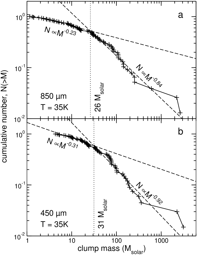
Figure 6: Cumulative mass functions for (a) the 77 clumps detected at 850 $\mu$m and (b) the 67 clumps detected at 450 $\mu$m (b), with masses calculated assuming T$=$35 K. The dashed lines represent fits to broken power laws, with slopes as labeled. The vertical dotted lines indicate the break points between the power laws.

To analyze the distribution of clump masses, we plot the cumulative number of clumps with masses greater than M, $N(>{\rm M})$, versus M. Figure 6 shows this cumulative mass function (CMF) for the 77 clumps detected at 850 $\mu$m and the 67 clumps detected at 450 $\mu$m, with masses calculated assuming a universal T${}_{\rm dust}=35$ K. We have not computed a mass function for the 850 $\mu$m clumps with variable-temperature masses due to concern that the omission of some clumps may introduce bias into the mass function, particularly if there is an intrinsic mass-temperature correlation not evident in our data. Omitting masses would be especially problematic in the case of the CMF, whose overall shape depends on the position of each individual clump. We fit each CMF with a broken power law, which takes the form $N(M)\propto M^{-\alpha}$ on either side of a break point (note that this $\alpha$ is not the same as the spectral index discussed earlier). The break point is also a parameter of the fit.

Both CMFs are well fit at the low-mass end by $\alpha\sim$ 0.2–0.3. At the high-mass end, where incompleteness should be less of a problem, both are well fit by $\alpha\sim$ 0.8–0.9. In both cases, the break point occurs above our estimated incompleteness thresholds of 15 M_⊙ and 25 M_⊙ in the 850 $\mu$m and 450 $\mu$m images, respectively, although we again emphasize the uncertainty in the positions of these thresholds. Both the degree of flattening at the low-mass end of the CMF and the position of the break point could be strongly influenced by incompleteness. Nonetheless, the existence of a break point above our estimated incompleteness thresholds suggests that the change in slope is a real property of the mass function of NGC 7538, not merely an artifact of incompleteness.

Both sections of the 450 $\mu$m CMF (Fig. 6b) are slightly steeper than their 850 $\mu$m counterparts (Fig. 6a). This may be a consequence of the fact that some of the 850 $\mu$m clumps resolve into two or more smaller, lower-mass clumps at 450 $\mu$m, shifting the distribution toward lower masses. The lower signal to noise ratio of the 450 $\mu$m map may also mean that it traces a smaller fraction of the mass of each clump, again biasing the mass function to lower masses. However, the flux calibrations are considerably less certain at 450 $\mu$m than at 850 $\mu$m, so it is difficult to be certain whether the difference in slopes between the 450 $\mu$m and 850 $\mu$m CMFs is real.

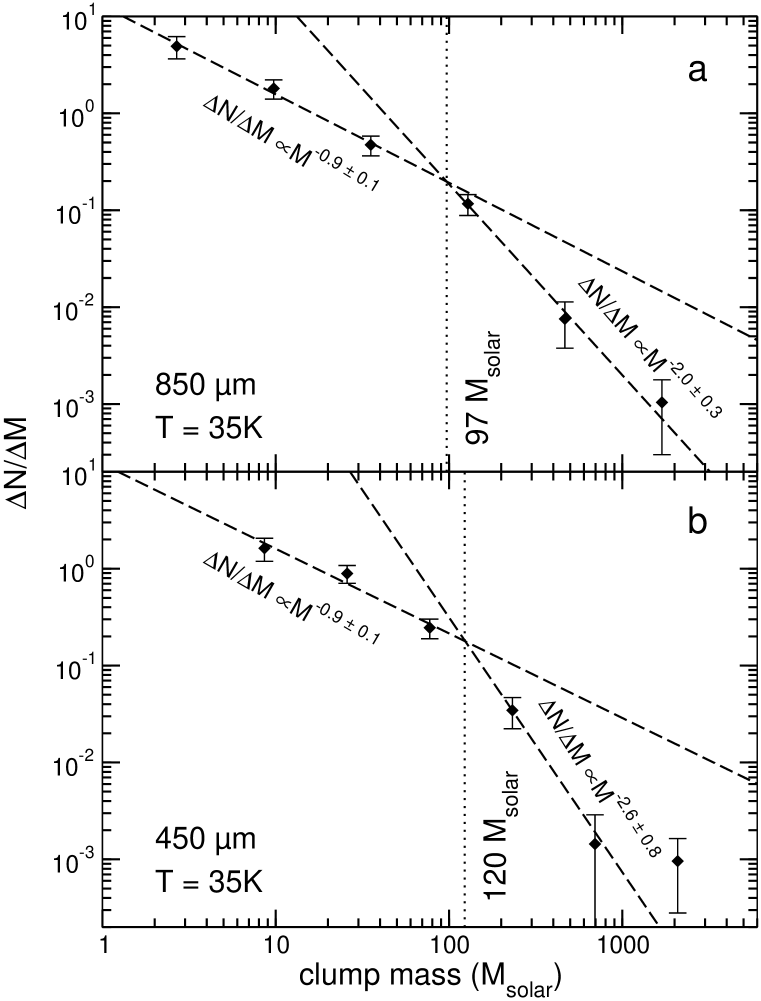
Figure 7: Differential mass functions for (a) the 77 clumps detected at 850 $\mu$m and (b) the 67 clumps detected at 450 $\mu$m, with masses calculated assuming T$=35$ K. The dashed lines represent fits to broken power laws, with slopes as labeled. The vertical dotted lines indicate the break points between the power laws.

A possible criticism of the cumulative mass function is that its shape is dependent on the position of each clump; there is no built-in averaging-out of uncertainties. With 77 clumps detected at 850 $\mu$m, we have enough objects to construct a differential mass function, $\Delta{\rm N}/\Delta{\rm M}$, where $\Delta$N is the number of clumps in the mass bin $\Delta{\rm M}$. Figure 7 plots such a function for the same sets of clumps as in Fig. 6. Again, we fit to two power laws of the form $\Delta{\rm N}/\Delta{\rm M}\propto{\rm M}^{-\gamma}$ on either side of a fitted break point, where $\gamma=\alpha+1$. At the low-mass end, we find $\gamma=0.9\pm 0.1$ for the clumps at both wavelengths. At the high-mass end, we find $\gamma=2.0\pm 0.3$ for the 850 $\mu$m clumps and $\gamma=2.6\pm 0.8$ for the 450 $\mu$m clumps. Again, the position of the break point should be viewed as considerably uncertain, particularly given how much higher it is for the differential mass functions than for the cumulative ones. Comparing the differential and cumulative mass functions of Figs. 6 and 7, we see that they all agree within the uncertainties at the high-mass end, where the data are most likely to be complete.

In all cases, lower incompleteness at higher clump masses means that the fit to the high-mass end of each mass function is more reliable than that to the low-mass end. The higher sensitivity and better calibration of the 850 $\mu$m data make the 850 $\mu$m clump mass estimates more reliable than the 450 $\mu$m ones. Finally, the straightforward interpretation of the uncertainties in the differential mass function leads us to trust it more than the cumulative mass function. Thus, our most reliable estimate of the power law exponent of the clump mass function in NGC 7538 is $\alpha=2.0\pm 0.3$, from the high-mass end of the 850 $\mu$m differential mass function.

4.3 Mass Functions and Turbulent Fragmentation

In Table High Mass Star Formation I: The Mass Distribution of Submillimeter Clumps in NGC 7538, we compare our results for NGC 7538 to similar mm and submm continuum studies of star-forming regions in which the mass function is fitted with a broken power law. All of these studies should be sensitive to the cold, dense dust and gas that forms the precursor structures to stars. The method of extracting the clumps and converting their integrated fluxes to masses is similar in all of the studies. Although both of the regions previously studied in this way ($\rho$ Oph and Orion B) have considerably lower average clump masses than NGC 7538, the shape of the mass function in all three regions is remarkably similar. In particular, the high-mass end of the mass function is well fit by an approximately Salpeter mass function ($\gamma=2.35$, Salpeter 1955). This agreement in the power-law exponents among the various clump mass functions suggests that the clump mass function is shaped by a common set of physical processes which operate self-similarly across a broad range of clump and parent cloud masses. This appears to be true despite the fact that the star-forming future of any given clump is usually not clear. In the low-mass regions, many of the clumps may form single stars, while others may form binaries and higher-order multiples. The NGC 7538 clumps span a range of masses, from those which may form only a single star, to those such as the IRS 1-3, 9, and 11 clumps, which will probably form small clusters of stars. Nevertheless, it appears that the Salpeter-like clump mass function may extend all the way from stellar-scale to cluster-scale submm clumps.

Turbulent theories of molecular cloud evolution suggest the mechanism by which this situation may come about. Hydrodynamic simulations of turbulent, self-gravitating gas have shown that, for a range of initial conditions corresponding to those typical of molecular clouds, the shape of the mass function is independent of the total mass of the cloud (Tilley & Pudritz, 2004). Taken together, the results of Table High Mass Star Formation I: The Mass Distribution of Submillimeter Clumps in NGC 7538 imply a shape for the clump mass function which does not vary substantially from cloud to cloud, and whose intrinsic scales (such as the position of the turnover) may be set by global properties of the parent molecular cloud, such as the total number of Jeans masses present.

In Table High Mass Star Formation I: The Mass Distribution of Submillimeter Clumps in NGC 7538, we also list those studies of the dust continuum clump mass function in Galactic star-forming regions in which the mass function was fitted with a single power law. In the case of Serpens, which is a nearby low-mass star forming region probed at small linear scales, the slope of the clump mass function is consistent with that of Salpeter. The remaining three regions (the Lagoon Nebula, KR 140, and RCW 106) are all more distant high-mass star-forming regions which were probed at spatial scales similar to or larger than those in our study of NGC 7538. The mass function in these regions is systematically more shallow than both the Salpeter mass function and those found in $\rho$ Oph, Orion B, and NGC 7538. Much of this discrepancy can be attributed to differences in analytical technique. If we fit the 850 $\mu$m clumps in NGC 7538, with a single power law, we find $\alpha=0.4\pm 0.2$, which is consistent with the results obtained in the other studies which used a single power law fit. However, as can be seen in Figures 6 and 7, none of our mass functions would be fit well by a single power law; there is a definite break point in the mass function, whether physical or an artifact of incompleteness. The mass functions of Tothill et al. (2002), Kerton et al. (2001), and Mookerjea et al. (2004) all show evidence of a similar break in the power law. If the mass functions for each of these regions were fit with a double power law, the derived exponent at the high mass end should increase and might then agree with the other studies given in Table High Mass Star Formation I: The Mass Distribution of Submillimeter Clumps in NGC 7538. Especially because the origin of the break is not well understood, we believe that a double power law whose break point is a fitted parameter is the most appropriate way to fit these mass functions. This issue will be examined further in Paper II.

Another common technique for measuring the clump mass function in star-forming regions is to extract the clumps from a CO spectral cube. Such studies typically find shallower mass functions than those which deal solely with the mm/submm clumps. Kramer et al. (1998) fitted single power law mass functions to the clumps extracted from ¹³CO (1$\rightarrow$0) and C¹⁸O (1$\rightarrow$0) maps of NGC 7538. In the two maps, they found $\gamma$ = 1.65 $\pm$ 0.05 and 1.79 $\pm$ 0.12, respectively, which agree within the uncertainties with our result of 2.0 $\pm$ 0.3 for the high-mass end of the 850 $\mu$m clump mass function. However, there appears to be statistically significant disagreement between the mass functions found in CO spectral line clump studies and mm/submm dust continuum studies generally. The mean slope of the high-mass end of the mm/submm mass functions fitted with two power laws (Table High Mass Star Formation I: The Mass Distribution of Submillimeter Clumps in NGC 7538) is $2.3\pm 0.1$, whereas the mean slope of the CO mass functions for the seven star-forming regions included in the study of Kramer et al. (1998) is $1.69\pm 0.02$. The CO and dust continuum studies span roughly the same range of clump masses: $\sim$10^-4–$10^{4}$ M_⊙ for the CO clumps and $\sim$10^-2–$10^{3}$ M_⊙ for the dust continuum studies. Thus, the discrepancy between the average slopes of the high mass ends of the CO and dust continuum mass functions appears to be real. An alternate interpretation is that the CO mass functions agree with the dust continuum mass functions of the Lagoon Nebula, KR 140, and RCW 106, which have a mean exponent of 1.6 $\pm$ 0.1. However, we note that, whereas the CO mass functions appear to be well fit by a single power law, the dust continuum mass functions are clearly not. If the high- and low-mass portions of the dust continuum mass functions in these regions were fitted separately, we believe the exponents of their high-mass power laws would be found to agree with those quoted in Table High Mass Star Formation I: The Mass Distribution of Submillimeter Clumps in NGC 7538 for $\rho$ Oph, Orion B, and NGC 7538, and to disagree with the exponents of the CO mass functions.

A possible explanation for the apparently real discrepancy between the CO spectral line and dust continuum mass functions is that the dust maps trace denser, more likely gravitationally bound clumps than the CO line maps, which may trace less dense, possibly transient structures (Motte et al. 2001, Tothill et al. 2002). This hypothesis could be tested by comparing CO and dust continuum maps of individual regions taken at similar resolutions and with sensitivity to structure on similar scales. Repeating this analysis at multiple resolutions and for a variety of regions would be very helpful. Freeze-out of CO in cooler and/or less massive clumps may also account for some of the discrepancy (Mitchell et al., 2001). Finally, some of the discrepancy may be attributable to the recovery of different types of structures from spectral cubes analyzed using algorithms like GAUSSCLUMPS (Stutzki & Güsten, 1990) or the 3D version of clumpfind, compared to those recovered from integrated intensity maps using algorithms like clfind2d, as here. To clfind2d, every integrated intensity peak represents a single clump, but the extra velocity information available in a spectral cube can allow GAUSSCLUMPS to decompose each peak into more than one clump along the line of sight, potentially producing systematically different mass functions.

What can we now conclude about the origin of the clump mass function and what that might imply for the origin of the stellar IMF? The five studies summarized in Table High Mass Star Formation I: The Mass Distribution of Submillimeter Clumps in NGC 7538 cover three different regions of star formation whose clump masses span five orders of magnitude, from $\sim$0.03 M_⊙ clumps in Johnstone et al. (2000b) to $\sim$3000 M_⊙ clumps in this work. In all cases, the high-mass end of the mass function, which is not strongly affected by incompleteness, is well-fit by a Salpeter-like power law with index $\sim$2.0–2.5. Similarly, the low-mass end of the mass function has a power law index of $\sim$0.9–1.5 in all cases. This agreement suggests that the processes which shape the clump mass function are self-similar, at least across five orders of magnitude in clump mass. In other words, the overall shape of the mass function is independent of the total mass of the molecular cloud, over the range of cloud masses studied. If there is an intrinsic scale in a cloud’s mass function, it appears to manifest as the position of the break point between the low and high mass ends. The results from the low-mass star-forming regions summarized in Table High Mass Star Formation I: The Mass Distribution of Submillimeter Clumps in NGC 7538 suggest that the break point may occur at $\sim$0.5–1.0 M_⊙, which roughly matches the break point in the stellar IMF (Kroupa, 2002). However, the appearance of a break point in the mass function of NGC 7538 suggests that this intrinsic scale of the clump mass function may scale with some global property of the parent cloud, such as its total mass or the number of Jeans masses present. If this is the case, then the mass function of clumps seen in high-mass regions may not simply be an extension of the high-mass end of the mass function seen in lower-mass regions. Instead, it may be a scaled-up version of the whole mass function seen in low-mass regions, including the break point. Indications of a similar high-mass break point can also be seen in the dust continuum clump mass functions of the Lagoon nebula (Tothill et al., 2002) and the molecular cloud complex RCW 106 (Mookerjea et al., 2004). However, in all of the dust continuum studies, the existence and/or the position of a break point could be a function of incompleteness. Continuum surveys at higher resolutions and sensitivities will be required to confirm the existence and position of the break point in the clump mass function.

Our observations of NGC 7538 are also consistent with theoretical and numerical studies of molecular clouds in which turbulent fragmentation sets the clump mass function, at least on large scales. In their simulations of several Jeans masses of self-gravitating, turbulent gas, Tilley & Pudritz (2004) found that turbulent fragmentation alone is sufficient to give rise to a Salpeter-like mass function with $\gamma=2.29$. A similar result was obtained by Gammie et al. (2003) for a magnetized, turbulent gas, who found $\gamma\simeq 2.3$ for both gravitationally bound and unbound clumps (and the ensemble of both). Padoan & Nordlund (2002) used an analytical approach to turbulent fragmentation to derive the same result ($\gamma=2.33$).

Our inability to estimate accurately the elapsed time since the onset of collapse in any given molecular cloud complicates this line of reasoning. For example, we cannot be entirely confident that the population of clumps in NGC 7538 is mostly unevolved; some coalescence of clumps may already have taken place, and some fraction of each clump’s mass may already have accreted onto one or more embedded protostars. The presence of a few very young, massive outflows in only the largest clumps and the absence of widespread maser activity suggests that star formation in NGC 7538 is in its very early stages, but only deep infrared surveys can address this issue adequately.

It is not yet clear what fraction of the clumps in NGC 7538 may form more than one star, and with what distribution of masses. This complicates any attempt to extrapolate a connection between stellar-mass clumps on linear scales of $\sim$ 0.02 pc and the clumps in our map, on scales of $\sim$ 0.2 pc. Nonetheless, we believe it is reasonable to interpret the early emergence of a Salpeter-like clump mass spectrum, on both large and small scales, as evidence that self-similar turbulent fragmentation may be sufficient to determine the final distribution of stellar masses, reducing the need to invoke other processes.

5 Summary

We have mapped the NGC 7538 massive star-forming region with high sensitivity at 850 $\mu$m and 450 $\mu$m. After processing the images to remove spurious large-scale structure, we used clfind2d to locate 77 clumps in the 850 $\mu$m image and 67 in the 450 $\mu$m image. Our calibrations take into account contamination from CO line emission, radio continuum emission, and the error beam at both wavelengths. Assuming a uniform dust temperature of 35 K, we find that the masses of the 850 $\mu$m and 450 $\mu$m clumps range from 1.2 to 2700 M_⊙ and 4 to 3100 M_⊙, respectively. We find a positive correlation between spectral index, $\alpha$, and submillimeter emission. This is the opposite result to that obtained by Font, Mitchell, & Sandell (2001), but the difference is entirely accounted for by differences in the techniques used to make the two maps. The positive correlation between high submm flux and high spectral index is likely due to the higher temperatures at the centers of massive cores, particularly those containing embedded protostars, but may also reflect spatial variations in the dust emissivity index, $\beta$. Using the spectral index map and the assumption of a constant dust emissivity index, $\beta$, we derive temperatures for 42 of the 77 clumps seen at 850 $\mu$m and use these in an alternative calculation of the clump masses.

Our most reliable analysis of the clump mass-radius relationship gives ${\rm M}\propto{\rm R}^{x}$ with $x\sim 1.5-2.1$. This result suggests that the clumps are characterized by a nearly constant column density, and that they probably have significant turbulent support. The similarity in the structures seen at 450 $\mu$m and 850 $\mu$m, which differ in resolution by a factor of two, suggests that the clumps we are seeing are coherent physical structures, and not superpositions of unrelated smaller objects.

We have derived the first set of mass functions for a large number of submm clumps in a single high-mass star-forming region. At the high-mass end where the data are not strongly affected by incompleteness, the mass function is approximately Salpeter. Our most reliable analysis gives an exponent of 2.0 $\pm$ 0.3 (compared to 2.35 for the Salpeter IMF) for the power law exponent of the high-mass end of the clump mass function, covering the range $\sim 100-3000$ M_⊙. The submm clump mass function of NGC 7538 agrees well with those found in $\rho$ Oph and Orion B, using similar analytical techniques. The range of clump masses covered by these studies plus our own spans five orders of magnitude. We find that the difference in the power law exponents of the CO and dust continuum clump mass functions is statistically significant. The dust continuum mass functions are typically steeper at the high-mass end than their CO counterparts, though a definitive explanation for this discrepancy is lacking. We interpret the similar shapes of the clump mass functions in both high-mass and low-mass star-forming regions as evidence for the self-similarity of the physical processes which set the clump mass function. We suggest that turbulent fragmentation may be the dominant process shaping the clump mass function in young star-forming regions. Finally, we interpret the early emergence of a Salpeter-like mass function in several young star-forming regions as evidence that late-stage processes such as competitive accretion and coalescence may not need to play a significant role in the generation of the stellar IMF.

Table 1: Two-Gaussian Beam Fits

		Primary Beam		First Error Beam
	Calibrator	Relative Amplitude	FWHM (arcsec)	Relative Amplitude	FWHM (arcsec)
850 $\mu$m	Uranus	0.95$\pm$0.08	14.2$\pm$0.5	0.05$\pm$0.03	30$\pm$5
	CRL 2688	0.9$\pm$0.1	15.1$\pm$0.9	0.04$\pm$0.04	40$\pm$10
450 $\mu$m	Uranus	0.9$\pm$0.1	8.5$\pm$0.6	0.06$\pm$0.03	27$\pm$4
	CRL 2688	0.9$\pm$0.2	9.2$\pm$0.7	0.08$\pm$0.04	30$\pm$5

Table 2: Properties of the 850 $\mu$m Clumps

Name	R.A.	Dec.	Reff	$S_{\rm peak}$	$S^{\rm int}_{850}$	$\langle{\alpha}\rangle$	$\langle{\rm T}_{d}\rangle$	M${}_{{\rm T}_{d}=35K}$	M${}_{{\rm T}_{d}}$	npsc
(NGC7538-)	(J2000)	(J2000)	(pc)	(Jy beam-1)	(Jy)		(K)	(M⊙)	(M⊙)
SMM1	23 12 49.8	+61 27 28	0.17	0.22$\pm$0.01	0.38$\pm$0.02	2.55	16	15.8$\pm$0.7	50$\pm$2	1
SMM2	23 12 52.1	+61 25 56	0.03	0.10$\pm$0.01	0.06$\pm$0.01	3.99	$\cdots$	2.4$\pm$0.5	$\cdots$	0
SMM3	23 12 53.2	+61 27 42	0.16	0.37$\pm$0.01	0.58$\pm$0.08	3.01	28	24$\pm$3	32$\pm$4	0
SMM4	23 12 54.6	+61 27 00	0.28	0.78$\pm$0.03	2.1$\pm$0.3	3.33	72	90$\pm$10	37$\pm$5	3
SMM5	23 12 55.1	+61 25 48	0.05	0.16$\pm$0.01	0.13$\pm$0.01	3.66	$\cdots$	5.2$\pm$0.5	$\cdots$	1
SMM6	23 12 55.4	+61 27 32	0.08	0.42$\pm$0.02	0.68$\pm$0.06	3.18	40	28$\pm$2	24$\pm$2	1
SMM7	23 12 56.2	+61 26 20	0.15	0.18$\pm$0.01	0.27$\pm$0.01	3.59	$\cdots$	11.2$\pm$0.5	$\cdots$	1
SMM8	23 12 56.8	+61 25 54	0.08	0.19$\pm$0.01	0.20$\pm$0.01	3.67	$\cdots$	8.4$\pm$0.3	$\cdots$	2
SMM9	23 12 58.7	+61 27 20	0.06	0.54$\pm$0.02	0.83$\pm$0.07	3.44	204	35$\pm$3	4.8$\pm$0.4	3
SMM10	23 12 59.0	+61 27 52	0.20	0.63$\pm$0.03	1.2$\pm$0.1	3.56	$\cdots$	51$\pm$6	$\cdots$	2
SMM11	23 12 59.3	+61 27 30	0.10	0.56$\pm$0.02	0.67$\pm$0.05	3.54	$\cdots$	28$\pm$2	$\cdots$	1
SMM12	23 13 00.4	+61 24 56	0.04	0.10$\pm$0.01	0.06$\pm$0.01	$\cdots$	$\cdots$	2.7$\pm$0.5	$\cdots$	0
SMM13	23 13 03.4	+61 27 52	0.12	0.17$\pm$0.01	0.20$\pm$0.04	3.50	$\cdots$	8$\pm$2	$\cdots$	0
SMM14	23 13 03.7	+61 24 28	0.12	0.16$\pm$0.01	0.19$\pm$0.04	$\cdots$	$\cdots$	8$\pm$2	$\cdots$	1
SMM15	23 13 05.4	+61 24 50	0.06	0.11$\pm$0.01	0.04$\pm$0.03	$\cdots$	$\cdots$	2$\pm$1	$\cdots$	0
SMM16	23 13 05.7	+61 28 04	0.14	0.25$\pm$0.01	0.39$\pm$0.01	3.45	219	16.2$\pm$0.6	2.09$\pm$0.07	1
SMM17	23 13 09.0	+61 23 56	0.13	0.17$\pm$0.01	0.23$\pm$0.01	3.78	$\cdots$	9.5$\pm$0.4	$\cdots$	0
SMM18	23 13 10.1	+61 28 18	0.34	1.09$\pm$0.04	3.3$\pm$0.5	3.49	$\cdots$	140$\pm$20	$\cdots$	3
SMM19	23 13 15.7	+61 29 10	0.26	0.85$\pm$0.03	2.1$\pm$0.3	3.13	35	90$\pm$10	90$\pm$10	7
SMM20	23 13 18.4	+61 29 28	0.16	0.39$\pm$0.02	0.73$\pm$0.03	3.06	30	31$\pm$1	37$\pm$1	1
SMM21	23 13 18.4	+61 28 50	0.25	0.25$\pm$0.01	0.70$\pm$0.03	2.64	17	29$\pm$1	81$\pm$4	2
SMM22	23 13 19.8	+61 25 20	0.27	1.05$\pm$0.04	3.0$\pm$0.4	3.13	35	120$\pm$20	120$\pm$20	6
SMM23	23 13 22.0	+61 24 54	0.28	0.84$\pm$0.03	2.6$\pm$0.3	3.53	$\cdots$	110$\pm$10	$\cdots$	0
SMM24	23 13 22.3	+61 29 12	0.22	0.32$\pm$0.01	0.91$\pm$0.04	2.57	16	38$\pm$2	116$\pm$6	3
SMM25	23 13 23.4	+61 31 06	0.06	0.12$\pm$0.01	0.09$\pm$0.01	$\cdots$	$\cdots$	3.7$\pm$0.3	$\cdots$	2
SMM26	23 13 24.5	+61 25 28	0.21	0.54$\pm$0.02	1.6$\pm$0.2	3.20	42	69$\pm$8	54$\pm$6	1
SMM27	23 13 25.1	+61 25 00	0.17	0.76$\pm$0.03	1.9$\pm$0.2	3.59	$\cdots$	81$\pm$8	$\cdots$	1
SMM28	23 13 25.6	+61 29 52	0.14	0.56$\pm$0.02	1.1$\pm$0.1	2.57	17	43$\pm$4	120$\pm$10	3
SMM29	23 13 25.6	+61 24 18	0.23	0.14$\pm$0.01	0.35$\pm$0.04	3.68	$\cdots$	15$\pm$1	$\cdots$	1
SMM30	23 13 26.8	+61 29 26	0.25	1.05$\pm$0.04	3.5$\pm$0.4	3.00	29	140$\pm$20	180$\pm$20	8
SMM31	23 13 27.0	+61 30 12	0.19	0.44$\pm$0.02	0.85$\pm$0.09	2.46	15	34$\pm$4	110$\pm$10	8
SMM32	23 13 28.4	+61 25 58	0.16	0.18$\pm$0.01	0.30$\pm$0.02	2.95	25	12.4$\pm$0.9	19$\pm$1	0
SMM33	23 13 29.0	+61 25 28	0.17	0.72$\pm$0.03	1.9$\pm$0.2	3.41	128	78$\pm$8	18$\pm$2	0
SMM34	23 13 29.5	+61 30 04	0.23	0.77$\pm$0.02	1.7$\pm$0.2	2.32	17	57$\pm$8	150$\pm$20	10
SMM35	23 13 29.8	+61 25 04	0.20	0.53$\pm$0.02	1.3$\pm$0.1	3.62	$\cdots$	53$\pm$6	$\cdots$	2
SMM36	23 13 30.1	+61 30 26	0.25	0.82$\pm$0.03	1.8$\pm$0.2	2.63	19	68$\pm$9	160$\pm$20	6
SMM37	23 13 30.6	+61 29 02	0.31	1.99$\pm$0.08	6.2$\pm$0.8	3.30	68	250$\pm$30	120$\pm$20	13
SMM38	23 13 31.5	+61 31 18	0.17	0.12$\pm$0.01	0.20$\pm$0.01	$\cdots$	$\cdots$	6.6$\pm$0.3	$\cdots$	1
SMM39	23 13 32.0	+61 26 56	0.16	0.15$\pm$0.01	0.24$\pm$0.01	$\cdots$	$\cdots$	9.9$\pm$0.2	$\cdots$	0
SMM40	23 13 33.7	+61 25 46	0.40	1.20$\pm$0.05	5.2$\pm$0.7	3.43	172	220$\pm$30	36$\pm$5	6
SMM41	23 13 33.7	+61 31 52	0.19	0.19$\pm$0.01	0.36$\pm$0.02	2.17	12	15.0$\pm$0.7	77$\pm$3	0
SMM42	23 13 34.2	+61 28 32	0.52	1.06$\pm$0.04	6.1$\pm$0.9	3.06	30	250$\pm$40	300$\pm$40	16
SMM43	23 13 35.6	+61 29 28	0.09	0.09$\pm$0.01	0.08$\pm$0.01	$\cdots$	$\cdots$	3.3$\pm$0.2	$\cdots$	3
SMM44	23 13 42.3	+61 31 36	0.21	0.54$\pm$0.02	1.0$\pm$0.1	2.97	26	43$\pm$5	63$\pm$7	0
SMM45	23 13 43.7	+61 31 34	0.23	0.54$\pm$0.02	0.9$\pm$0.1	3.11	34	38$\pm$5	39$\pm$5	0
SMM46	23 13 44.5	+61 26 48	0.67	14.1$\pm$0.6	53$\pm$8	3.50	$\cdots$	2200$\pm$300	$\cdots$	4
SMM47	23 13 44.8	+61 29 12	0.18	0.20$\pm$0.01	0.29$\pm$0.03	3.28	329	11$\pm$1	0.9$\pm$0.1	0
SMM48	23 13 45.3	+61 28 10	0.68	18.1$\pm$0.7	70$\pm$10	3.44	$\cdots$	2700$\pm$400	$\cdots$	8
SMM49	23 13 45.3	+61 25 50	0.14	0.21$\pm$0.01	0.33$\pm$0.01	1.48	8	13.6$\pm$0.4	143$\pm$4	1
SMM50	23 13 48.4	+61 25 50	0.23	0.20$\pm$0.01	0.54$\pm$0.01	2.16	12	22.5$\pm$0.5	118$\pm$2	3
SMM51	23 13 49.2	+61 29 10	0.18	0.16$\pm$0.01	0.31$\pm$0.08	2.66	17	13$\pm$4	35$\pm$9	4
SMM52	23 13 53.4	+61 27 00	0.37	0.96$\pm$0.04	4.2$\pm$0.6	3.31	66	180$\pm$20	80$\pm$10	9
SMM53	23 13 53.9	+61 28 52	0.06	0.10$\pm$0.01	0.03$\pm$0.01	$\cdots$	$\cdots$	1.4$\pm$0.3	$\cdots$	0
SMM54	23 13 56.4	+61 27 08	0.30	0.81$\pm$0.03	2.6$\pm$0.3	3.37	93	110$\pm$10	35$\pm$5	15
SMM55	23 13 56.7	+61 27 50	0.17	0.15$\pm$0.01	0.24$\pm$0.01	$\cdots$	$\cdots$	10.0$\pm$0.2	$\cdots$	0
SMM56	23 13 58.9	+61 31 28	0.37	0.68$\pm$0.03	2.6$\pm$0.4	3.08	32	110$\pm$10	120$\pm$20	5
SMM57	23 13 59.5	+61 30 54	0.18	1.25$\pm$0.05	2.6$\pm$0.3	3.29	59	110$\pm$10	59$\pm$7	3
SMM58	23 14 00.6	+61 28 02	0.06	0.11$\pm$0.01	0.07$\pm$0.01	$\cdots$	$\cdots$	2.8$\pm$0.3	$\cdots$	1
SMM59	23 14 00.9	+61 29 50	0.04	0.09$\pm$0.01	0.05$\pm$0.01	$\cdots$	$\cdots$	2.1$\pm$0.2	$\cdots$	0
SMM60	23 14 02.0	+61 27 20	0.59	3.9$\pm$0.2	14$\pm$2	3.45	225	600$\pm$90	80$\pm$10	4
SMM61	23 14 02.0	+61 30 16	0.14	0.81$\pm$0.03	1.0$\pm$0.1	3.24	48	41$\pm$4	27$\pm$3	4
SMM62	23 14 02.3	+61 29 34	0.06	0.12$\pm$0.01	0.10$\pm$0.01	$\cdots$	$\cdots$	4.0$\pm$0.2	$\cdots$	0
SMM63	23 14 05.9	+61 31 00	0.26	1.45$\pm$0.06	3.5$\pm$0.5	3.32	69	140$\pm$20	64$\pm$8	1
SMM64	23 14 05.9	+61 30 10	0.16	0.34$\pm$0.01	0.69$\pm$0.03	3.18	40	29$\pm$1	24.4$\pm$0.9	1
SMM65	23 14 06.2	+61 31 30	0.27	0.75$\pm$0.03	2.0$\pm$0.2	3.24	49	80$\pm$10	54$\pm$7	3
SMM66	23 14 08.4	+61 29 44	0.20	0.33$\pm$0.01	0.71$\pm$0.05	3.15	37	29$\pm$2	28$\pm$2	1
SMM67	23 14 08.4	+61 30 00	0.10	0.29$\pm$0.01	0.36$\pm$0.07	3.10	33	15$\pm$3	16$\pm$3	1
SMM68	23 14 11.7	+61 31 46	0.15	0.12$\pm$0.01	0.20$\pm$0.01	$\cdots$	$\cdots$	8.41$\pm$0.08	$\cdots$	2
SMM69	23 14 12.3	+61 26 14	0.06	0.09$\pm$0.01	0.03$\pm$0.01	$\cdots$	$\cdots$	1.4$\pm$0.3	$\cdots$	0
SMM70	23 14 15.0	+61 25 54	0.06	0.13$\pm$0.01	0.10$\pm$0.01	3.20	43	4.1$\pm$0.3	3.1$\pm$0.2	1
SMM71	23 14 18.1	+61 26 00	0.08	0.13$\pm$0.01	0.12$\pm$0.01	$\cdots$	$\cdots$	4.9$\pm$0.3	$\cdots$	1
SMM72	23 14 22.8	+61 29 50	0.06	0.11$\pm$0.01	0.03$\pm$0.01	$\cdots$	$\cdots$	1.2$\pm$0.2	$\cdots$	0
SMM73	23 14 26.7	+61 31 34	0.06	0.09$\pm$0.01	0.03$\pm$0.01	$\cdots$	$\cdots$	1.3$\pm$0.3	$\cdots$	0
SMM74	23 14 29.2	+61 31 30	0.06	0.11$\pm$0.01	0.08$\pm$0.01	$\cdots$	$\cdots$	3.13$\pm$0.07	$\cdots$	0
SMM75	23 14 29.7	+61 28 52	0.09	0.15$\pm$0.01	0.14$\pm$0.01	4.12	$\cdots$	5.9$\pm$0.1	$\cdots$	0
SMM76	23 14 32.5	+61 31 14	0.06	0.10$\pm$0.01	0.06$\pm$0.01	$\cdots$	$\cdots$	2.3$\pm$0.6	$\cdots$	2
SMM77	23 14 36.7	+61 27 46	0.07	0.13$\pm$0.01	0.11$\pm$0.01	3.24	49	4.5$\pm$0.2	3.0$\pm$0.1	0

Table 3: Properties of the 450 $\mu$m Clumps

Name	R.A.	Dec.	Reff	$S_{\rm peak}$	$S^{\rm int}_{450}$	M${}_{{\rm T}_{d}=35K}$	npsc
(NGC7538-)	(J2000)	(J2000)	(pc)	Jy beam-1	(Jy)	(M⊙)
SMM4A	23 12 52.6	+61 26 36	0.13	1.7$\pm$0.2	3.7$\pm$0.3	15$\pm$1	0
SMM3A	23 12 53.7	+61 27 44	0.10	1.5$\pm$0.2	2.6$\pm$0.3	11$\pm$1	0
SMM4B	23 12 55.1	+61 26 58	0.24	3.6$\pm$0.4	22$\pm$2	93$\pm$7	2
SMM6A	23 12 55.1	+61 27 34	0.14	2.0$\pm$0.2	5$\pm$1	22$\pm$6	1
SMM8A	23 12 56.2	+61 25 52	0.12	1.2$\pm$0.1	2.28$\pm$0.01	9.49$\pm$0.05	1
SMM9A	23 12 57.1	+61 27 14	0.17	2.3$\pm$0.3	8.8$\pm$0.4	37$\pm$2	3
SMM10A	23 12 59.3	+61 27 50	0.27	3.2$\pm$0.4	19$\pm$3	80$\pm$10	1
SMM9B	23 12 59.3	+61 27 16	0.16	2.5$\pm$0.3	8$\pm$1	33$\pm$5	2
SMM16A	23 13 05.7	+61 27 54	0.18	1.2$\pm$0.1	4.7$\pm$0.4	19$\pm$2	1
SMM18A	23 13 10.1	+61 28 22	0.34	5.7$\pm$0.7	35$\pm$6	150$\pm$30	2
SMM19A	23 13 15.9	+61 29 10	0.26	4.0$\pm$0.5	18$\pm$3	70$\pm$10	4
SMM20A	23 13 18.7	+61 29 28	0.20	1.8$\pm$0.2	7.7$\pm$0.7	32$\pm$3	1
SMM22B	23 13 20.4	+61 25 24	0.23	4.5$\pm$0.5	18$\pm$3	80$\pm$10	5
SMM21A	23 13 20.4	+61 28 44	0.13	1.1$\pm$0.1	2.46$\pm$0.01	10.24$\pm$0.04	0
SMM22A	23 13 21.2	+61 25 12	0.19	3.7$\pm$0.4	14$\pm$2	59$\pm$8	1
SMM23A	23 13 22.6	+61 24 56	0.19	3.7$\pm$0.4	17$\pm$2	69$\pm$9	0
SMM26C	23 13 23.7	+61 25 58	0.07	1.0$\pm$0.1	1.0$\pm$0.4	4$\pm$2	1
SMM26A	23 13 24.3	+61 25 20	0.15	2.5$\pm$0.3	10$\pm$2	40$\pm$10	0
SMM26B	23 13 24.8	+61 25 38	0.21	2.2$\pm$0.3	9.8$\pm$0.4	41$\pm$2	1
SMM27B	23 13 25.4	+61 25 02	0.19	3.4$\pm$0.4	18$\pm$2	80$\pm$10	1
SMM30A	23 13 25.6	+61 29 14	0.18	2.5$\pm$0.3	8$\pm$1	34$\pm$4	0
SMM28A	23 13 26.2	+61 29 50	0.17	1.5$\pm$0.2	5.7$\pm$0.8	24$\pm$3	1
SMM28B	23 13 26.5	+61 30 06	0.17	1.6$\pm$0.2	5.0$\pm$0.3	21$\pm$1	6
SMM30B	23 13 27.3	+61 29 26	0.18	4.4$\pm$0.5	16$\pm$2	68$\pm$9	5
SMM37A	23 13 27.6	+61 29 00	0.22	5.0$\pm$0.6	24$\pm$4	100$\pm$20	2
SMM27A	23 13 27.6	+61 24 40	0.14	1.5$\pm$0.2	4.0$\pm$0.6	17$\pm$2	0
SMM33A	23 13 29.5	+61 25 26	0.26	3.4$\pm$0.4	23$\pm$4	90$\pm$20	0
SMM34B	23 13 29.5	+61 30 04	0.15	2.3$\pm$0.3	5$\pm$2	23$\pm$7	4
SMM34A	23 13 29.5	+61 29 40	0.09	0.9$\pm$0.1	1.29$\pm$0.03	5.4$\pm$0.1	1
SMM34C	23 13 30.1	+61 30 14	0.13	1.9$\pm$0.2	4$\pm$1	17$\pm$5	4
SMM36B	23 13 30.1	+61 30 46	0.08	0.9$\pm$0.1	1.14$\pm$0.02	4.73$\pm$0.07	2
SMM36A	23 13 30.4	+61 30 28	0.15	3.3$\pm$0.4	8$\pm$1	34$\pm$4	3
SMM37B	23 13 30.9	+61 29 02	0.25	10$\pm$1	47$\pm$8	200$\pm$30	5
SMM42B	23 13 31.5	+61 28 18	0.16	1.8$\pm$0.2	5.9$\pm$0.5	24$\pm$2	1
SMM35A	23 13 32.0	+61 25 00	0.19	2.1$\pm$0.3	9.2$\pm$0.7	38$\pm$3	3
SMM40A	23 13 33.7	+61 25 42	0.42	5.9$\pm$0.7	60$\pm$10	230$\pm$40	4
SMM42C	23 13 34.0	+61 28 30	0.40	4.5$\pm$0.5	44$\pm$8	180$\pm$30	13
SMM42A	23 13 34.0	+61 27 50	0.13	0.9$\pm$0.1	2.16$\pm$0.03	9.0$\pm$0.1	0
SMM44A	23 13 39.8	+61 31 22	0.11	0.8$\pm$0.1	1.8$\pm$0.2	7.3$\pm$0.8	0
SMM45A	23 13 43.7	+61 31 38	0.23	2.4$\pm$0.3	10.9$\pm$0.6	45$\pm$2	0
SMM46A	23 13 44.8	+61 26 48	0.63	80$\pm$10	500$\pm$100	2300$\pm$400	2
SMM48A	23 13 45.3	+61 28 10	0.64	73$\pm$8	800$\pm$100	3000$\pm$600	6
SMM47A	23 13 45.3	+61 29 14	0.11	1.0$\pm$0.1	2.04$\pm$0.03	8.5$\pm$0.1	1
SMM48C	23 13 47.0	+61 28 54	0.16	1.3$\pm$0.2	4.2$\pm$0.7	17$\pm$3	3
SMM46B	23 13 49.8	+61 26 58	0.35	11$\pm$1	80$\pm$10	310$\pm$60	1
SMM48B	23 13 51.2	+61 28 48	0.18	1.2$\pm$0.1	4.70$\pm$0.02	19.53$\pm$0.08	1
SMM56A	23 13 51.4	+61 31 22	0.08	0.9$\pm$0.1	1.2$\pm$0.5	5$\pm$2	0
SMM56C	23 13 53.7	+61 31 26	0.11	1.3$\pm$0.2	2.39$\pm$0.04	9.9$\pm$0.2	0
SMM52B	23 13 54.2	+61 27 00	0.17	5.1$\pm$0.6	19$\pm$3	80$\pm$10	4
SMM52A	23 13 54.5	+61 26 50	0.27	4.9$\pm$0.6	24$\pm$4	100$\pm$20	7
SMM56D	23 13 55.1	+61 31 32	0.10	1.6$\pm$0.2	3.06$\pm$0.02	12.75$\pm$0.07	1
SMM54A	23 13 56.4	+61 27 12	0.23	4.2$\pm$0.5	18$\pm$3	70$\pm$10	11
SMM56E	23 13 56.7	+61 31 36	0.13	2.4$\pm$0.3	5$\pm$1	22$\pm$5	0
SMM57A	23 13 59.8	+61 30 52	0.24	6.6$\pm$0.8	25$\pm$4	100$\pm$20	0
SMM56B	23 13 59.8	+61 31 26	0.24	2.8$\pm$0.3	15$\pm$1	62$\pm$4	5
SMM60B	23 14 00.9	+61 27 02	0.25	8$\pm$1	42$\pm$7	180$\pm$30	10
SMM60D	23 14 02.0	+61 27 20	0.26	27$\pm$3	90$\pm$10	360$\pm$60	2
SMM61A	23 14 02.3	+61 30 16	0.17	4.6$\pm$0.6	9$\pm$1	37$\pm$5	2
SMM60A	23 14 05.0	+61 26 58	0.32	6.5$\pm$0.8	39$\pm$7	160$\pm$30	1
SMM64A	23 14 05.6	+61 30 12	0.18	1.7$\pm$0.2	5.9$\pm$0.4	24$\pm$2	0
SMM65A	23 14 05.9	+61 31 28	0.27	3.3$\pm$0.4	17$\pm$3	70$\pm$10	1
SMM63A	23 14 06.2	+61 31 00	0.30	7.1$\pm$0.9	33$\pm$6	140$\pm$20	1
SMM66A	23 14 09.2	+61 29 48	0.15	1.3$\pm$0.2	3.88$\pm$0.03	16.1$\pm$0.1	0
SMM67A	23 14 09.5	+61 30 06	0.19	1.2$\pm$0.1	5.57$\pm$0.06	23.1$\pm$0.2	0
SMM60C	23 14 11.4	+61 27 18	0.15	1.2$\pm$0.1	3.3$\pm$0.2	13.6$\pm$0.9	0
SMM75A	23 14 30.0	+61 29 00	0.12	1.2$\pm$0.1	2.5$\pm$0.4	11$\pm$2	0
SMM77A	23 14 36.4	+61 27 44	0.11	0.9$\pm$0.1	1.6$\pm$0.2	6.7$\pm$0.8	0

Table 4: Submm Clumps Associated with IRS Sources

IRS Source	Associated
Number	Submm Clump
1, 2, & 3	SMM48
4	SMM37
5	SMM34
9	SMM60
11	SMM46

Table 5: Power Law Fits to (Sub)Millimeter Clump Mass Functions

	$\lambda$	HPBW	Fitted Mass		Mbreak	CMF Exponents		DMF Exponents
Region	($\mu{\rm m}$)	(pc)	Range (M⊙)	Nfit	(M⊙)	$\alpha_{\rm low}$	$\alpha_{\rm high}$	$\gamma_{\rm low}$	$\gamma_{\rm high}$	Ref.
Double Power Law Fits
NGC 7538	850	0.21	1.2–2700	77	26, 97	0.23	0.84	0.9 $\pm$ 0.1	2.0 $\pm$ 0.3	1
NGC 7538	450	0.11	4–3100	67	31, 120	0.31	0.92	0.9 $\pm$ 0.1	2.6 $\pm$ 0.8	1
$\rho$Oph	1300	0.0085	0.05–3.2	58	0.5	0.5	1.5	1.5	2.5	2
$\rho$Oph	850	$\sim$0.025	0.02–6.3	55	0.6	0.5	1.0-1.5	1.5	2.0-2.5	3
NGC 2068/2071	850	0.02	$\sim$ 0.3–5	70	0.7	0.5	1.1	1.5	2.1	4
Orion B	850	0.03	0.06–30.3	75	$\sim 1.0$	0.5	1.5	1.5	2.5	5
Single Power Law Fits
Serpens	3000	$\sim$0.0075	$\sim$ 0.4–32	26	$\cdots$	$\cdots$	1.1	$\cdots$	2.1	6
Lagoon (M8)	450 & 850	0.13	6.3–43	$\sim$ 50	$\cdots$	$\cdots$	0.7 $\pm$ 0.6	$\cdots$	1.7 $\pm$ 0.6	7
KR 140	850	0.22	0.7–130	25	$\cdots$	$\cdots$	0.49 $\pm$ 0.04	$\cdots$	1.49 $\pm$ 0.04	8
RCW 106	1200	0.42	$\sim$ 40–104	95	$\cdots$	$\cdots$	0.6 $\pm$ 0.3	$\cdots$	1.6 $\pm$ 0.3	9

References. — (1) This paper; (2) Motte, André, & Neri (1998); (3) Johnstone et al. (2000b); (4) Motte et al. (2001); (5) Johnstone et al. (2001); (6) Testi & Sargent (1998); (7) Tothill et al. (2002); (8) Kerton et al. (2001); (9) Mookerjea et al. (2004)

References

- Bonnell et al. (1997) Bonnell, I. A., Bate, M. R., Clarke, C. J., & Pringle, J. E. 1997, MNRAS, 285, 201
- Bonnor (1956) Bonnor, W. G. 1956, MNRAS, 116, 351
- Crampton, Georgelin, & Georgelin (1978) Crampton, D., Georgelin, Y. M., & Georgelin, Y. P. 1978, A&A, 66, 1
- Davis et al. (1998) Davis, C. J., Moriarty-Schieven, G., Eislöffel, J., Hoare, M. G., & Ray, T. P. 1998, AJ, 115, 1118
- Ebert (1955) Ebert, R. 1955, Z. Astrophys., 37, 217
- Elmegreen & Falgarone (1996) Elmegreen, B. G. & Falgarone, E. 1996, ApJ, 471, 816
- Elmegreen (1997) Elmegreen, B. G. 1997, ApJ, 486, 944
- Emerson (1995) Emerson, D. T. 1995, in ASP Conf. Ser. 75, Multi-Feed Systems for Radio Telescopes, ed. D. T. Emerson & J. M. Payne (San Francisco: ASP), 309
- Font, Mitchell, & Sandell (2001) Font, A. S., Mitchell, G. F., Sandell, G. 2001, ApJ, 555, 950
- Gammie et al. (2003) Gammie, C. F., Lin, Y., Stone, J. M., & Ostriker, E. C. 2003, ApJ, 592, 203
- Hildebrand (1983) Hildebrand, R. H. 1983, QJRAS, 24, 267
- Hogerheijde & Sandell (2000) Hogerheijde, M. R. & Sandell, G. 2000, ApJ, 534, 880
- Israel (1977) Israel, F. P. 1977, A&A, 59, 27
- Jenness et al. (2000) Jenness, T., Holland, W. S., Chapin, E., Lightfoot, J. F., & Duncan, W. D. 2000, in ASP Conf. Ser. 216, Astronomical Data Analysis Software and Systems IX, ed. N. Manset, C. Veillet, & D. Crabtree (San Francisco: ASP), 559
- Jenness & Lightfoot (1998) Jenness, T., & Lightfoot,J. F. 1998, in ASP Conf. Ser. 145, Astronomical Data Analysis Software and Systems VII, ed. R. Albrecht, R. N. Hook, & H. A. Bushouse (San Francisco: ASP), 216
- Johnstone et al. (2000a) Johnstone, D. J., Wilson, C. D., Moriarty-Schieven, G., Creighton, J. G., & Gregersen, E. 2000a, ApJS, 131, 505
- Johnstone et al. (2000b) Johnstone, D. J., Wilson, C. D., Moriarty-Schieven, G., Joncas, G., Smith, G., Gregersen, E., & Fich, M. 2000b, ApJ, 545, 327
- Johnstone et al. (2001) Johnstone, D. J., Fich, M., Mitchell, G. F., Moriarty-Schieven, G. 2001, ApJ, 559, 307
- Kameya et al. (1990) Kameya, O., Morita, K.-I., Kawabe, R., & Ishiguro, M. 1990, ApJ, 355, 562
- Kerton et al. (2001) Kerton, C. R., Martin, P. G., Johnstone, D., & Ballantyne, D. R. 2001, ApJ, 552, 601
- Klessen, Burkert, & Bate (1998) Klessen, R. S., Burkert, A., & Bate. M. R. 1998, ApJ, 501, L205
- Kramer et al. (1998) Kramer, C., Stutzki, J., Röhrig, R., & Corneliussen, U. 1998, A&A, 329, 249
- Kroupa (2002) Kroupa, P. 2002, Science, 295, 82
- Larson (1981) Larson, R. B. 1981, MNRAS, 194, 809
- McLaughlin & Pudritz (1996) McLaughlin, D. E. & Pudritz, R. E. 1996, ApJ, 469, 194
- Mitchell et al. (2001) Mitchell, G. F., Johnstone, D., Moriarty-Schieven, G., Fich, M., Tothill, N. F. H. 2001, ApJ, 556, 215
- Mookerjea et al. (2004) Mookerjea, B., Kramer, C., Nielbock, M., & Nyman, L.-Å. 2004, A&A, 426, 119
- Moreno & Chavarria-K. (1986) Moreno, M. A., Chavarria-K., C. 1986, A&A, 161, 130
- Motte et al. (2001) Motte, F., André, P., Ward-Thompson, D., Bontemps, S. 2001, A&A, 372, L41
- Motte, André, & Neri (1998) Motte, F., André, P., & Neri, R. 1998, A&A, 336, 150
- Motte, Schilke, & Lis (2003) Motte, F., Schilke, P., & Lis, D.C. 2003, ApJ, 582, 277
- Padoan & Nordlund (2002) Padoan, P. & Nordlund, Å. 2002, ApJ, 576, 870
- Rots et al. (1981) Rots, A. H., Dickel, H. R., Forster, J. R., & Goss, W. M. 1981, ApJ, 245, L15
- Salpeter (1955) Salpeter, E. E. 1955, ApJ, 121, 161
- Sandell, Wright, & Forster (2003) Sandell, G., Wright, M., & Forster, J. R. 2003, ApJ, 590, L45
- Sandell & Sievers (2004) Sandell, G., & Sievers, A. 2004, ApJ, 600, 269
- Seaquist et al. (2004) Seaquist, E., Yao, L., Dunne, L., & Cameron, H. 2004, MNRAS, 349, 1428
- Stutzki & Güsten (1990) Stutzki, J. & Güsten, R. 1990, ApJ, 356, 513
- Testi & Sargent (1998) Testi, L. & Sargent, A. I. 1998, ApJ, 508, L91
- Tilley & Pudritz (2004) Tilley, D. A. & Pudritz, R. E. 2004, MNRAS, 353, 769
- Tothill et al. (2002) Tothill, N. F. H., White, G. J., Matthews, H. E., McCutcheon, W. H., McCaughrean, M. J., Kenworthy, M. A. 2002, ApJ, 580, 285
- Werner et al. (1979) Werner, M. W., Becklin, E. E., Gatley, I., Matthews, K., Neugebauer, G., & Wynn-Williams, C. G. 1979, MNRAS, 188, 463
- Williams, de Geus, & Blitz (1994) Williams, J. P., de Geus, E. J., & Blitz, L. 1994, ApJ, 428, 693
- Wynn-Williams, Becklin, & Neugebauer (1974) Wynn-Williams, C. G., Becklin, E. E., & Neugebauer, G. 1974, ApJ, 187, 473
- Young et al. (2004) Young, C. H., et al. 2004, ApJS, 154, 396
- Zheng et al. (2001) Zheng, X.-W., Zhang, Q., Ho. P. T. P., & Pratap, P. 2001, ApJ, 550, 301