MCG–6-30-15: Long Timescale X-Ray Variability, Black Hole Mass and AGN High States

Abstract

We present a detailed study of the long-timescale X-ray variability of the Narrow Line Seyfert 1 Galaxy (NLS1) MCG–6-30-15, based on eight years of frequent monitoring observations with the Rossi X-ray Timing Explorer. When combined with the published short timescale XMM-Newton observations, we derive the powerspectral density (PSD) covering 6 decades of frequency from $\sim 10^{-8}$ to $\sim 10^{-2}$Hz. As with NGC4051, another NLS1, we find that the PSD of MCG–6-30-15 is a close analogue of the PSD of a Galactic Black Hole X-ray binary system (GBH) in a ‘high’ rather than a ‘low’ state. As with NGC4051 and the GBH Cygnus X-1 in its high state, a smoothly bending model is a better fit to the PSD of MCG–6-30-15, giving a derived break frequency of $7.6^{+10}_{-3}\times 10^{-5}$ Hz. Assuming linear scaling of break frequency with black hole mass, we estimate the black hole mass in MCG–6-30-15 to be $\sim 2.9^{+1.8}_{-1.6}\times 10^{6}$$M_{\odot}$.

Although, in the X-ray band, it is one of the best observed Seyfert galaxies, there has as yet been no accurate determination of the mass of the black hole in MCG–6-30-15. Here we present a mass determination using the velocity dispersion ($M_{\rm BH}-\sigma_{*}$) technique and compare it with estimates based on the width of the $\rm H\alpha$ line. Depending on the calibration relationship assumed for the $M_{\rm BH}-\sigma_{*}$ relationship, we derive a mass between 3.6 and 6 $\times 10^{6}$$M_{\odot}$, consistent with the mass derived from the PSD.

Using the newly derived mass and break timescale, and revised reverberation masses for other AGN from Peterson et al. (2004), we update the black hole mass/break timescale diagram. The observations are still generally consistent with narrow line Seyfert 1 galaxies having shorter break timescales, for a given mass, than broad line AGN, probably reflecting a higher accretion rate. However the revised, generally higher, masses (but unchanged break timescales) are also consistent with perhaps all of the X-ray bright AGN studied so far being high state objects. This result may simply be a selection effect, based on their selection from high-flux X-ray all sky catalogues, and their consequent typically high X-ray/radio ratios, which indicate high state systems.

1 Introduction

It is now reasonably well established that the X-ray powerspectral densities (PSDs) of AGN are broadly similar to those of galactic black hole X-ray binary systems (GBHs) (M^cHardy, 1988; Edelson & Nandra, 1999; Uttley et al., 2002; Markowitz et al., 2003; M^cHardy et al., 2004). The PSDs are described by powerlaws of the form $P(\nu)\propto\nu^{\alpha}$, where $P(\nu)$ is the power at frequency $\nu$, but $\alpha$ varies with frequency (see Section 3.2.1 for details). At high frequencies the PSDs of both AGN and GBHs are steep (slope, $\alpha,\sim-2$) but below a break frequency, $\nu_{B}$, typically at a few Hz for GBHs, they flatten to a slope of $\alpha\sim-1$. To first order, the break timescale scales linearly with the black hole mass but there is still considerable uncertainty in the mass/break timescale relationship and hence in our understanding of the physical similarities between AGN and GBHs.

The uncertainty arises largely because GBHs occur in several distinct states (e.g. see McClintock & Remillard, 2003). Most commonly they are found in the so-called ‘low’ state where their X-ray fluxes are low and their medium energy (2-10 keV) X-ray spectra are hard. The second most common state is the ‘high’ state where their fluxes are high and their 2-10 keV spectra are soft. The PSDs of GBHs in these two states are quite different. In the low state, there is a second break, about a decade below the high frequency break (Nowak et al., 1999). Below the lower frequency break the PSD flattens further to a slope of zero. In the high state there is no second break and the PSD continues with slope $\sim-1$ to very low frequencies (Cui et al., 1997). In addition the break from slope $\sim-2$ to slope $\sim-1$ occurs at a higher frequency in the high state than in the low state ($\sim 15$Hz cf $\sim 3$Hz in the best studied GBH Cyg X-1). Before comparing AGN with GBHs it is therefore important to know whether the AGN is a high or low state system.

Based on their 2-10 keV X-ray spectra, it has generally been assumed that AGN are the equivalent of low state GBHs. However, although the high frequency ($\nu>10^{-6}$Hz) parts of many AGN PSDs are now reasonably well determined, the lower frequencies are, in general, not well determined and so it is not usually possible to be sure whether AGN are the analogues of low or high state GBHs. In general it is not possible to determine whether there is a second, lower frequency, break or not. The difficulty in determining the low frequency shape of AGN PSDs has been in obtaining well sampled lightcurves stretching over sufficiently long timescales. For an assumed linear scaling of break timescale with mass, we require well sampled lightcurves of a few years duration to detect the second, lower, break in a black hole of mass $\sim 10^{6}$ $M_{\odot}$.

Prior to the launch of RXTE in November 1995 it was not possible to obtain long timescale lightcurves of sufficient quality but, since early 1996 we (M^cHardy et al., 1998; Uttley et al., 2002; M^cHardy et al., 2004), and others (Edelson & Nandra, 1999; Markowitz et al., 2003), have been monitoring a small sample of AGN, typically observing each AGN once every 2 days, and so are able to determine the shape of the low frequency PSD to high precision. Using these observations we (M^cHardy et al., 2004) recently showed that the PSD of the narrow line Seyfert 1 (NLS1) galaxy NGC 4051 was, in fact, identical to that of a high, rather than low state GBH and so provided the first definite confirmation of a high state AGN. Markowitz et al. (2003) plotted the black hole mass against the timescales associated with well measured PSD breaks, some from slope $\sim-2$ to $\sim-1$ and some from slope $\sim-1$ to $\sim 0$. They claimed that there was a linear relationship between the two parameters. With a somewhat larger sample we (M^cHardy et al., 2004) plotted the black hole mass against the timescale associated with the specific PSD break from slope $\sim-2$ to $\sim-1$ for a sample of AGN. We found that the best fit to all of the AGN together had a slope flatter than unity and did not extrapolate to either the high or low state break timescales of Cyg X-1. However we noted that the break timescales associated with broad line Seyfert 1 galaxies were, for a given black hole mass, generally longer than those for those objects usually classed as NLS1s. NLS1s are probably not a distinct class of object but, more likely, just lie at one end of a spectrum of AGN properties, characterised perhaps by a higher accretion rate. However taking the crude broad/narrow line distinction which is commonly used in the literature, we note that a linear BH-mass/break-timescale relationship fits broad line AGN and Cyg X-1 in the low state, and a displaced linear relationship fits the NLS1s and Cyg X-1 in the high state. We therefore suggested that there is no fixed break timescale/mass relationship which fits all AGN but that the break timescale/mass relationship may actually vary in response to one or more other factors, which might be accretion rate or black hole spin.

In order to test and clarify the above hypothesis, it is necessary to place AGN on the break timescale/mass plane with high precision and to determine whether they are high or low state analogues. There are very few AGN for which the X-ray observations are extensive enough to make the latter determination possible and a particularly important object is therefore the Seyfert galaxy MCG–6-30-15. Although MCG–6-30-15 is not always described as an NLS1, it has many of the properties commonly associated with NLS1s, ie rapid X-ray variability and relatively narrow permitted emission lines (FWHM 1700 km $\rm s^{-1}$ (Pineda et al., 1980) c.f. the 2000 km $\rm s^{-1}$ limit which is usually quoted for NLS1s). In this paper we therefore class MCG–6-30-15 as a NLS1, like NGC4051.

Figure 1: Long Term RXTE 2-10 keV lightcurve of MCG–6-30-15. Each data point represents an observation of $\sim 1$ ks.

MCG–6-30-15 is one of the best studied X-ray bright Seyfert galaxies. It was the galaxy in which the first detection of a relativistically broadened X-ray iron line was made, providing direct evidence for the existence of a massive black hole (Tanaka et al., 1995). We have monitored it extensively with the Rossi X-ray Timing Explorer (RXTE) and have presented its long timescale PSD (Uttley et al., 2002), based on 3 years of observations (1996-1999). From that early, limited, dataset Uttley et al. (2002) were able to show that a simple unbroken powerlaw was not a good fit to the PSD (at greater than 99 percent rejection confidence) but that a broken powerlaw did provide a good fit (rejection confidence 33 percent). However it was not possible to determine, with any accuracy, the low frequency PSD slope. If they assumed a powerlaw of slope -1, Uttley et al. were able to derive a break frequency in the PSD at $\sim$few $\times 10^{-5}$Hz and to estimate the high frequency powerlaw slope ($\sim-2$). Thus Uttley et al. were unable to distinguish a high from a low state system, or measure the break timescale with high precision, although they preferred the high state interpretation as a low state interpretation implied a luminosity close to the Eddington limit. Vaughan et al. (2003) have subsequently published a detailed study of the short timescale X-ray variability of MCG–6-30-15 using observations from XMM-Newton. These observations are insufficient, on their own, to determine the low frequency PSD slope but, by also assuming a low frequency PSD slope of -1, they have determined the break frequency to be $\sim 1\times 10^{-4}$Hz.

In this paper (Section 2) we present our full RXTE observations, of 8 years duration, and consisting of over 800 separate observations, compared to 100 in Uttley et al. (2002). In Section 3 we combine these RXTE observations with the published XMM-Newton observations and derive a PSD of excellent quality covering over 6 decades of frequency from $<10^{-8}$ to $>10^{-2}$Hz. We determine accurately the shape of the PSD below the $\sim 10^{-4}$Hz break and we thereby show that MCG–6-30-15 is, like NGC4051 (M^cHardy et al., 2004), the analogue of a high state GBH. Using our improved determination of the low frequency PSD shape, we slightly refine the break timescale.

The most widely accepted method of determining black hole masses in Seyfert galaxies is that of reverberation mapping (e.g. Peterson, 2001) but this technique has not yet been applied to MCG–6-30-15. The best current estimate of the BH mass in MCG–6-30-15 is $\sim 1\times 10^{6}\rm M_{\odot}$ (Uttley et al., 2002).

That mass is based on an estimated bulge mass of $3\times 10^{9}\rm M_{\odot}$ (Reynolds, 2000) and on the correlation between black hole mass and galactic bulge mass presented by Wandel (1999), where he claims that Seyfert galaxies have a lower black hole mass, for a given bulge mass, than was claimed in the original relationship of Magorrian et al. (1998). In a later paper Wandel (2002) revises the black hole mass/bulge ratio to 0.0015 and shows that Seyfert galaxies fit the same relationship as normal galaxies. Using the revised ratio, and the estimated bulge mass from Reynolds (2000), the revised black hole mass would be $4.5\times 10^{6}\rm M_{\odot}$.

An upper limit to the black hole mass of $10^{7}$$M_{\odot}$has been derived by Morales & Fabian (2002), using a method based on balancing the radiative and gravitational forces acting on outflowing warm absorber clouds. However it has recently become clear that the successful technique of determining black hole masses from the central velocity dispersion of the galaxy bulge can be applied to active, as well as quiescent, galaxies by observing the width of the Caii triplet in the far red, where the AGN continuum is not dominant (Ferrarese et al., 2001). In Section 4 we report the determination of the black hole mass in MCG–6-30-15 from central velocity dispersion measurements. For comparison (Section 5) we also estimate the BH mass from the width of the $\rm H\beta$ emission line and the continuum flux at 5100Å, using empirical relations from Kaspi et al. (2000). With greater error, we also estimate (Section 6) the BH mass using the ‘photoionisation’ method (Wandel et al., 1999).

In Section 7 we discuss the implications of our results for the comparison of AGN and GBHs.

2 X-RAY OBSERVATIONS AND DATA REDUCTION

2.1 RXTE

The RXTE observations discussed here consist of our own monitoring observations, which have continued since 1996, and two ‘long looks’ in August 1997 and July 1999 which we have obtained from the RXTE archive. The monitoring observations cover timescales from less than a day to $\sim$few years and the long looks cover timescales from $\sim$days to $\sim$minutes.

2.1.1 Monitoring Observations

The RXTE monitoring observations, of typically $\sim$1 ks duration, were made and analysed in exactly the same way as for NGC4051 (M^cHardy et al., 2004). Prior to 2000, we used a quasi-logarithmic sampling pattern, covering all timescales, but in order to improve the S/N on our resulting PSDs, we then increased our coverage. From 2000 onwards, our typical observation frequency has been once every two days. In addition, to sample properly the higher frequencies, we observed once every 6 hours for 2 months in 2000. Each observation, of $\sim 1$ksec duration, contributes one flux point to the monitoring lightcurve. We do not attempt to split the monitoring data into higher time resolution bins.

The observations were made with the Proportional Counter Array (PCA) which consists of 5 Xenon-filled proportional counter units (PCUs). We extracted the Xenon 1 (top) layer data from all PCUs that were switched on during the observation as layer 1 provides the highest S/N for photons in the energy range 2-20 keV where the flux from AGN is strongest. We used FTOOLS v4.2 for the reduction of the PCA data. We used standard ‘good time’ data selection criteria, i.e. target elevation $>10^{\circ}$, pointing offset $<0.01^{\circ}$, time since passage through the South Atlantic Anomaly of $>30$min and standard threshold for electron contamination. We calculated the model background in the PCA with the tool PCABACKEST v2.1 using the L7 model for faint sources. PCA response matrices were calculated individually for each observation using PCARSP V2.37, taking into account temporal variations of the detector gain and the changing number of detectors used. Fluxes in the 2-10 keV band were then determined using XSPEC, fitting a simple powerlaw with variable slope but with absorption fixed at the Galactic level of $4.06\times 10^{20}$ cm^-2 (Elvis et al., 1989). The errors in the flux are scaled directly from the observed errors in the measured count rate.

As with NGC4051, we produce a lightcurve in flux units, rather than raw observed counts/sec, so that we may use together data from periods when the number, and gain, of the PCUs changes. The resulting lightcurve, from 1996 to 2004, is presented in Fig. 1.

From the monitoring observations we make three lightcurves. The 6-hr sampled lightcurve consists of the 2 months of observations 4 times per day. The 2-d sampled lightcurve consists of the period from 2000 onwards where sampling is once every 2 days. The total lightcurve consists of all of the observations since 1996, but when used in the PSD analysis it is always heavily binned to 28 or 56-d resolution.

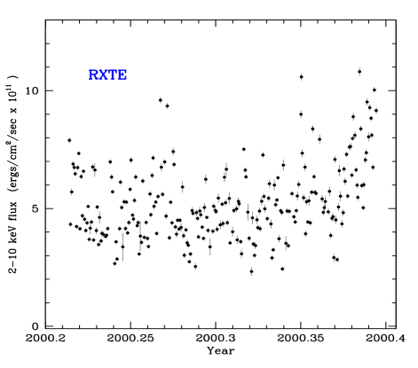
Figure 2: The 2-10 keV RXTE lightcurve of MCG–6-30-15 covering the two-month period of four observations per day. Each data point again represents an observation of $\sim 1$ ks.

2.1.2 Long Looks

There have been two long looks with RXTE , one in August 1997 and the other in July 1999. The total duration of each observation was about 9 days, consisting of continuous segments of $\sim 3$ksec, separated by gaps of approximately equal length caused by earth occultation. The August 1997 observations have been published by Lee et al. (2000) who have carried out a preliminary analysis of their variability properties. Lee et al. (2000) claim a break in the powerspectrum at $\sim 4-5\times 10^{-6}$Hz. Nowak & Chiang (2000) have analysed the same dataset, together with ASCA observations, and claim that the resultant PSD resembles that of a GBH in a low state. The claim that the PSD is flat below $10^{-5}$Hz, has a slope of approximately -1 from $10^{-5}$Hz to $\sim 10^{-4}$Hz and, above $\sim 10^{-4}$Hz it steepens to a slope of -2. Neither Lee et al. or Nowak and Chiang carry out simulations to determine the validity of their PSDs. Uttley et al. (2002) do carry out simulations and conclude that that although there is a break in the PSD of MCG–6-30-15, the model of Nowak and Chiang can be rejected at 99 percent confidence and that there is significant power in the PSD below $10^{-5}$Hz. A time-series analysis of the July 1999 observations has not yet been published.

The two long looks were analysed in exactly the same way as the monitoring observations, except that we retained 16s time resolution. As the July 1999 lightcurve has not previously been published, we include it here (Fig. 3) and, for the convenience of the reader, we also include the August 1997 lightcurve which has previously been published by Lee et al.

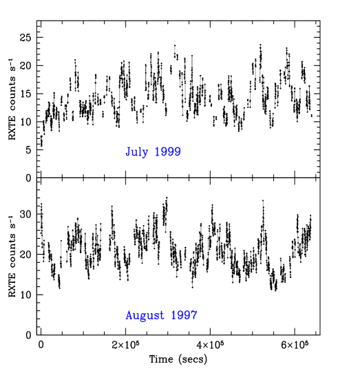
Figure 3: RXTE background-subtracted lightcurve of MCG–6-30-15 in the 2-10 keV energy band, with 128s time bins. The lightcurves are shown as histogram segments. Gaps are left where there are no data. Bottom panel is the August 1997 observation and top panel is the July 1999 observation. In both cases the time is measured since the start of the observation.

2.2 XMM-Newton

The XMM-Newton timing observations of MCG–6-30-15 have been discussed extensively by Vaughan et al. (2003) to which we refer readers for a detailed discussion. For the convenience of readers, we reproduce their lightcurve here (Fig 4).

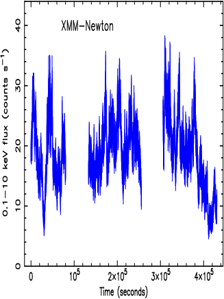
Figure 4: XMM-Newton background-subtracted lightcurve of MCG–6-30-15 in the 0.1-10 keV energy band, with 20s time bins, using data from the PN CCDs.

3 PSD Determination

The method used to determine the PSD is the same Monte Carlo simulation-based modelling technique (Uttley et al., 2002), psresp, which we employed in the analysis of the combined XMM-Newton and RXTE observations of NGC4051 (M^cHardy et al., 2004). This method is able to take account of non-uniform sampling and gaps in the data.

3.1 Long Timescale PSD

A variety of datasets are available for determination of the overall PSD but the RXTE monitoring observations provide the only information on timescales longer than $\sim$days. We therefore begin by fitting a simple power law to the PSD from the combined 6-hr, 2-d and total RXTE lightcurves. We retain the intrinsic 6-hr and 2-d resolution for the first two lightcurves but bin the total lightcurve up to 28-d resolution.

The resulting PSD is well fitted (fit probability = 68 percent) by a slope of $0.9\pm 0.15$ (90 percent confidence intervals are used throughout this paper). In Uttley et al. (2002) we describe how we determine the goodness of fit from the simulations. A fit probability of 68 percent means that the model is rejected at 32 percent confidence. The fit is shown in Fig. 5. For a GBH in the low-hard state, we do not expect the region of slope $\sim-1$ to extend for more than one or 1.5 decades, before flattening to a slope near zero. Although this fit would not be very sensitive to breaks near to the end of the frequency spectral range covered, nonetheless the fit to a simple power law, of slope close to $-1$ over approximately three decades, from $\sim 10^{-8}$ to $\sim 10^{-5}$ Hz, suggests that MCG–6-30-15 is the analogue of an XRB in a high-soft state rather than in a low-hard state.

Figure 5: Long timescale RXTE PSD of MCG–6-30-15. The PSD is well fitted (P=68 percent) by a simple powerlaw of slope $0.9\pm 0.25$ over three decades. The underlying undistorted model PSD is shown by the smooth continuous line. The distorted model for each of the three datasets, together with its errors, is shown by the individual points. The observed dirty PSD is given by the jagged lines.

3.2 Combined Long and Short Timescale PSD

3.2.1 RXTE monitoring observations and XMM-Newton 4-10 keV observations

In order to determine properly the overall long and short timescale PSD, and hence measure any break frequency and high frequency PSD slope, and refine measurements of the low frequency PSD slope, we must combine the RXTE monitoring observations with observations which sample shorter timescales.

Both the RXTE long looks and the XMM-Newton long observations provide information on shorter timescales. The RXTE long looks provide a good determination of the PSD on timescales shorter than the length of the individual segments ($\sim 3000$s). However on timescales between $\sim 3000$s and $\sim$few days, the PSD is distorted by the many gaps in the datasets. Our psresp analysis software is able to cope with those gaps, but they do give the software considerable work to do as the dirty PSD differs a good deal from any likely underlying true PSD. Thus the errors are larger than if there are fewer gaps. The XMM-Newton data are continuous and so the XMM-Newton PSD suffers negligibly from distortion. However the sensitivity of XMM-Newton is less than that of RXTE in the 2-10 keV range, which is the only energy band in which the long timescale PSD is determined. Nonetheless, the long XMM-Newton observations of MCG–6-30-15, which total approximately three times as long as those of NGC4051, do allow a reasonable determination of the high frequency PSD.

As discussed in M^cHardy et al. (2004), the mean photon energy of the 4-10 keV XMM-Newton band is approximately the same as that of the RXTE 2-10 keV band. In order to derive a PSD of uniform energy at all frequencies we have therefore included the 4-10 keV XMM-Newton PSD with the RXTE monitoring datasets described above in our PSD simulation process. The high-soft state PSD of Cyg X-1 is better described by a bending powerlaw model than a sharply broken powerlaw model, and the PSD of NGC4051 is also slightly better fit by the bending powerlaw model

$$P(\nu)=A\nu^{\alpha_{L}}\,\left(1+\left(\frac{\nu}{\nu_{b}}\right)^{(-\alpha_{H}+\alpha_{L})}\right)^{-1}\,$$

where $\alpha_{L}$ and $\alpha_{H}$ are the low and high frequency powerlaw slopes respectively and $\nu_{b}$ is the bend, or break, frequency. As stated in the Introduction, here we use the convention that a slope decreasing towards high frequencies will be defined by $P(\nu)\propto\nu^{\alpha}$ where $\alpha$ is a negative number, eg $\alpha=-2$.

We fit this model to the combined RXTE and XMM-Newton observations and the result is shown in Figs. 6 and  7. In Fig. 6 we plot the log of power vs. the log of frequency, as in Fig. 5. In both of these figures the observed dirty PSDs from the various constituent lightcurves are given by the jagged lines. The model, distorted by the effects of sampling, red noise leak and aliasing, is given by the points with errorbars, and the underlying, undistorted, model is given by the smooth dashed line. In Fig. 7 we unfold the observed dirty PSD from the distorting effect of the sampling in order to produce the closest approximation that we can to the true underlying PSD. Thus displacements of the observed PSD from the model distorted PSD are translated into displacements from the best-fit underlying model PSD. The technique is identical to that used to deconvolve energy spectra from count rate (ie instrumental) spectra in standard X-ray spectral fitting. In this case the error is translated onto the observed datapoints and the underlying best-fit model is shown as a continuous line. As in standard X-ray spectral fitting, the position of the datapoints does depend on the shape of the assumed, best-fitting, model. Note that in Fig. 7 we plot frequency $\times$power so that a horizontal line would represent $Power(\nu)\propto\nu^{-1}$ and equal power in each decade. Similar plots for NGC4051, NGC3516 and Cyg X-1 are shown in Fig.18 of M^cHardy et al. (2004).

The combined PSD is well fitted (P=45 percent) by this model with low frequency slope $\alpha_{L}=-0.8^{+0.4}_{-0.16}$, high frequency slope $\alpha_{H}=-1.98^{+0.32}_{-0.40}$ and break frequency $\nu_{B}=6.0^{+10}_{-5}\times 10^{-5}$Hz. A sharply broken powerlaw, although tolerable, is not such a good fit (P=14 percent) but the best fit parameters are similar to those of the smoothly bending model ($\alpha_{L}=-0.8$, $\alpha_{H}=-1.74$ and $\nu_{B}=3.2\times 10^{-5}$Hz). As is often the case, the break frequency is slightly lower for the sharply bending model than for the smoothly bending model but, in this case, the errors are not well determined. (Note that our software performs a simple grid search so the values given here are those of the minimum point on the grid and so may differ very slightly from the optimum values which may lie slightly off any particular grid point.) The confidence contours for these parameters are shown in Figs. 8, 9 and 10.

The break frequency for Cyg X-1, assuming a high state, bending powerlaw model, is $22.9\pm 1.5$Hz (M^cHardy et al., 2004) (or $13.9\pm 0.8$Hz for a sharply breaking high state model). Assuming linear scaling of black hole mass with frequency, and a black hole mass of 10$M_{\odot}$for Cyg X-1  (Herrero et al., 1995), we derive a black hole mass for MCG–6-30-15 of $3.6^{+18}_{-2}\times 10^{6}$$M_{\odot}$.

Figure 6: Combined 2-10 keV RXTE and 4-10 keV XMM-Newton PSD of MCG–6-30-15. The lines and datapoints are as described in Fig. 5.

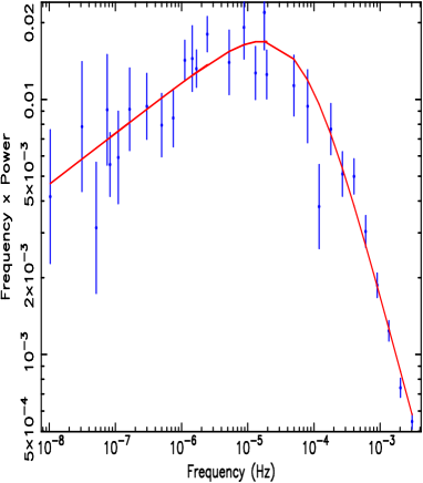
Figure 7: Unfolded combined 2-10 keV RXTE and 4-10 keV XMM-Newton PSD of MCG–6-30-15. Here the errors have been translated onto the datapoints and the continous line represents the best-fit underlying PSD. Note that here we plot frequency $\times$Power. See text for details.

Figure 8: 68 percent, 90 percent and 99 percent confidence contours for high frequency slope, $\alpha_{H}$, and break frequency, $\nu_{B}$, for bending powerlaw fit to the combined RXTE and XMM-Newton 4-10 keV PSD shown in Fig. 6. Note we plot $-\alpha_{H}$.

Figure 9: 68 percent, 90 percent and 99 percent confidence contours for low frequency slope, $\alpha_{L}$, and break frequency, $\nu_{B}$, for bending powerlaw fit to the combined RXTE and XMM-Newton 4-10 keV PSD shown in Fig. 6. Note we plot $-\alpha_{L}$

Figure 10: 68 percent, 90 percent and 99 percent confidence contours for low and high frequency slopes, $\alpha_{L}$ and $\alpha_{H}$ respectively for bending powerlaw fit to the combined RXTE and XMM-Newton 4-10 keV PSD shown in Fig. 6. Note we again plot $-\alpha_{L}$ and $-\alpha_{H}$.

We note that, although consistent within the errors with the break frequency derived by Vaughan et al. (2003) using purely XMM-Newton observations, our break frequency is slightly lower. The reason for the difference is that Vaughan et al. were unable to measure the PSD slope below the break and so assumed a value of -1. However our data show that the slope is actually slightly flatter, which leads to a lower break frequency.

3.2.2 RXTE monitoring observations and low energy XMM-Newton observations

In M^cHardy et al. (2004) we refined our determination of the break frequency in NGC4051 by combining RXTE monitoring observations with continuous XMM-Newton observations in the 0.1-2 keV band, where the break is better defined. We assumed that the break frequency was independent of energy. We have carried out the same procedure here (again taking proper account of the different PSD normalisations between the 0.1-2 and 2-10 keV bands) and find that $\alpha_{L}=-0.8^{+0.2}_{-0.1}$, $\alpha_{H}=-2.5^{+0.3}_{-0.4}$ and $\nu_{B}=7.6^{+10}_{-3}\times 10^{-5}$Hz. The fit probability is 67 percent. Apart from the steeper high energy slope which is well known at low energies (Vaughan et al., 2003; M^cHardy et al., 2004), the other fit parameters are very similar to those obtained when using the RXTE and XMM-Newton 4-10 keV observations. Thus within the errors, we find no evidence for a change of break frequency with photon energy. The implied black hole mass is more tightly constrained by the smaller errors on the break frequency and is $2.9^{+1.8}_{-1.6}\times 10^{6}$$M_{\odot}$.

We fitted a sharply breaking powerlaw model to the combined RXTE and XMM-Newton 0.1-2 keV data. As with the combined RXTE and 4-10 keV XMM-Newton data, the fit parameters are almost exactly the same as for the bending powerlaw model, but the fit probability is worse (19 percent). The fact that a bending powerlaw is a better fit than a sharply bending powerlaw to the PSD of MCG–6-30-15, as it is to the PSD of Cyg X-1in its high state, strengthens our conclusion that MCG–6-30-15 is the analogue of a GBH in the high, rather than low, state.

3.2.3 RXTE monitoring observations and RXTE long looks

We have also determined the overall PSD shape by including the RXTE long looks binned up to 128s time resolution with the RXTE monitoring observations, and also including a very high frequency PSD ($>10^{-3}$Hz) made from the individual segments of the RXTE long looks. The fit parameters are approximately the same as in the combined RXTE and XMM-Newton fit ($\alpha_{L}=-0.8^{+0.5}_{-0.15}$, $\alpha_{H}=-2.1^{+0.4}_{-0.6}$ and $\nu_{B}=5.0^{+8}_{-4}\times 10^{-5}$Hz). The fit is formally good (P=74 percent) but the errors are rather large because of the difficulty of coping with the many gaps in the RXTE long look lightcurves.

3.3 Search for a second, lower frequency, break

We searched for a second, lower frequency break, using the RXTE and XMM-Newton 4-10 keV data. We assumed a low state PSD model, fixing the slope below the lower break at 0, and the slope between the lower and upper breaks at -0.8, i.e. the value we measure in the same frequency range assuming a high state model. We allowed the two break frequencies and the slope above the upper break to vary. The best fit frequency for the higher break and for the slope above the higher break was the same as in our high state fit and the best fit for the lower break frequency ($6\times 10^{-9}$Hz) was almost at the end of the fitting range. The fit probability was 43 percent. In Fig. 11 we show the 68 percent, 90 percent and 99 percent confidence ranges for the two break frequencies. As the typical ratio of the two break frequencies for a low state GBH is between 10 and 30, we plot, as dashed straight lines, the limits corresponding to a ratios of 10 and of 100. The best fit ratio is over 1000, but a ratio of 100 is just within the edge of the 90 percent confidence region.

We repeated the above analysis after fixing the intermediate slope at $-1.0$ and obtained almost identical frequency ratios although the high break frequency was then about half a decade higher in frequency.

On the basis of its PSD, the above analysis strongly suggest that MCG–6-30-15 is the analogue of a high state GBH, although a low state cannot be entirely ruled out.

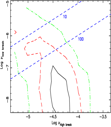
Figure 11: Confidence contours for the high and possible low break frequencies. The 68 percent contour is solid, the 90 percent contour is dashed and the 99 percent contour is dot-dashed. The straight dashed lines, with labels of 10 and 100 respectively, indicate those ratios between the high and possible low break frequencies. The fits assume a break below the low frequency break of 0 and an intermediate slope between the low and high frequency breaks of 0.8. Both break frequencies were allowed to vary, as was the slope above the upper break, which was measured at $1.95\pm 0.3$.

4 Mass Determination: Absorption Line Velocity Dispersion

As discussed in the Introduction, the mass of the black hole in MCG–6-30-15 is not well determined. In particular there have been no reverberation mapping observations, and no measurement of the stellar velocity dispersion, the two techniques widely regarded as giving the most reliable measurement of black hole masses. However a reliable measurement of the mass in MCG–6-30-15 is important for any discussion of mass/timescale scalings in AGN and for any discussions of whether AGN are in low or high states. In this section we therefore present stellar velocity dispersion measurements from which we estimate the black hole mass. In subsequent sections (Sec 5 and Sec 6) we present secondary determinations of the black hole mass, based on the width of the $\rm H\beta$ emission line and on photoionisation calculations. We find that all these optically based mass determination methods give consistent answers.

4.1 Observations

The observations of MCG–6-30-15 described here were taken by the service programme of the 3.6m Anglo-Australian Telescope on 2002 June 5. The RGO Spectrograph was used, with the 25cm camera plus the 1200R grating (blazed at 7500 Å). The detector is an EEV2 CCD, windowed to $600\times 4096$ pixels for the science observations and $150\times 4096$ pixels for the standard stars. A slit width of $1^{\prime\prime}$ (0.15mm) was chosen, resulting in a spectrum of resolution R $\sim 9500$ covering a wavelength range of 1000 Å. The slit was placed along the major axis of the galaxy, at a position angle of $116^{\circ}$.

The measured widths of the Caii triplet lines are used to estimate the black hole mass. At the redshift of MCG–6-30-15, $z=0.00775$, the Caii lines are shifted to $\lambda\lambda 8566,8610$ and $8731$ Å, and therefore the central wavelength was chosen to be $8620$ Å. The total wavelength coverage of 1000 Å, spanning the wavelength range $8120-9120$ Å, allows accurate determination of the continuum on either side of the lines, and therefore correct measurement of the line widths.

Observations of late-type giant stars, which have very narrow lines, and which dominate the stellar light of nearby galaxy bulges, were performed in order to measure the instrumental broadening and provide templates for the cross-correlation analysis. The K0 iii standard stars HD 117927 and HD 118131 were observed, with the same set-up and wavelength coverage as MCG–6-30-15, since the rest wavelength of the Caii triplet ($\lambda\lambda 8498,8542,8662$Å) lies within the wavelength range covered.

Dedicated flat field exposures were taken before and after the science and standard star observations, for accurate de-fringing, and argon and neon arc spectra were taken for the wavelength calibration.

4.2 Data Reduction

The raw data were reduced with IRAF using standard bias subtraction, flat fielding and cosmic ray removal techniques. At the red wavelengths observed here, the EEV2 CCD suffers from fringing at a level of $\sim 5$ percent. A comparison of the extracted science spectra with equivalent spectra taken from the flat field frames showed that the fringes were efficiently removed from the science frames, and did not contribute any spurious features. Curvature in the spatial direction was rectified using bright night sky lines in the object frames. The narrow window used for the standard star observations meant that in this case, rectification was unnecessary. The continua of MCG–6-30-15  and the standard stars were sufficiently bright that curvature of the spectra in the dispersion direction could be traced and rectified. The total exposure time for MCG–6-30-15  was 1 hr, broken into two 30min integrations. Wavelength calibration was performed using the arc exposures bracketing each science frame. This calibration was checked by measuring the resulting wavelength of night sky emission lines, and no further correction was required.

The nuclear spectrum of MCG–6-30-15  was extracted from the central 5.6 pixels of the trace, which corresponds to a $2.4^{\prime\prime}\times 1^{\prime\prime}$ aperture. To be compatible with the $M_{\rm BH}-\sigma_{*}$ relation defined by Ferrarese & Merritt (2000), the length of this aperture was chosen to correspond to $r_{e}/8$, where $r_{e}$ is the effective radius of the galaxy, measured from the profile of the spectral data, compressed along the dispersion direction. We note however that the choice of extraction aperture has only a very small effect on the results obtained (Ho, private communication). Sky subtraction was performed using regions either side of the galaxy, 50 pixels ($21.5^{\prime\prime}$) wide, at a distance of 50 pixels ($21.5^{\prime\prime}$) from the centre of the galaxy. The resulting spectrum is shown in Fig. 12, normalised by a spline fit to the continuum to emphasize the emission and absorption features.

Figure 12: Normalised spectra of MCG–6-30-15 (top panel) and a template star (bottom), with the position of the calcium triplet feature and broad Oi $\lambda 8446$ emission line marked.

In a similar analysis, Filippenko & Ho (2003) detect Paschen emission lines in the spectrum of NGC 4395, adjacent to each of the calcium absorption features. For MCG–6-30-15, there is perhaps a suggestion of a broad Paschen 15 line at $\sim 8615$Å, but it is not conclusive. Even if present, the strength of such a line is very small compared to those detected in NGC 4395, and as such, would not significantly affect our results.

4.3 Data Analysis

The calcium absorption features in a galaxy spectrum are broadened compared to those of an individual star due to the bulk motion of the stars in the galaxy. The extent of this Doppler broadening is related to the mass of the central black hole, giving rise to the observed tight relationship between the two quantities. The region of the galaxy spectrum of MCG–6-30-15  containing the calcium triplet is therefore cross-correlated with the equivalent region of the K0iii stellar templates using the IRAF task fxcor. The task fits a spline function to the continuum of each input spectrum, and cross-correlates the resulting features, giving as output a velocity measurement, due to the redshift of MCG–6-30-15, and a velocity width, due to the Doppler effect of the motion of stars in the galaxy caused by the gravitational influence of the black hole.

The width of the cross-correlation peak function calculated by fxcor measures the combined Doppler and instrumental broadening, therefore in order to ascertain the Doppler broadening alone, the stellar templates themselves were broadened using a Gaussian of various widths, and cross-correlated with the unbroadened templates. The width of the Gaussian which gave rise to a cross-correlation peak width equal to that of MCG–6-30-15  provides our measurement of the true velocity dispersion of the galaxy. We found that broadening the stellar templates by 11 pixels gave the best match to the cross-correlation peak width of MCG–6-30-15. The velocity dispersion of the spectra is $8.5\,{\rm km\,s}^{-1}\,{\rm pix}^{-1}$, giving a velocity dispersion for MCG–6-30-15 of $\sigma=93.5\,{\rm km\,s}^{-1}$.

The statistical errors on this measurement are very small, and therefore do not provide a realistic estimate of the true errors involved. Ferrarese et al. (2001) estimate that the systematic uncertainties involved in making such measurements are of order 15 percent. We therefore undertook a number of tests in order to ascertain the likely error in our result. First, since we have three standard star observations (two of HD 117927 and one of HD 118131), each spectrum was broadened in turn and cross-correlated with the two unbroadened stellar templates to estimate the variation due to the use of differing standards. The results usually varied by less than one percent, and never more than two percent. Secondly, to assess the possible impact of the proximity of the Oi line to the first feature in the calcium triplet, we restrict the region of the spectra used in the cross-correlation analysis to that containing only two of the three calcium absorption lines. By changing the wavelength range over which the cross-correlation analysis is performed, a maximum variation of $\pm 4$ percent in the peak width was measured. Thirdly, we vary the amount of smoothing of the stellar templates required to match the result from MCG–6-30-15, and find that all the results of the above tests are easily bracketed by taking a Gaussian width of $11\pm 1$ pixels, which is equivalent to $\sigma=93.5\pm 8.5\,{\rm km\,s}^{-1}$ ($\pm 9.1$ percent). We therefore take this as our conservative estimate of the error in our measurement, and note that this is small compared to the uncertainty in the relationship between this quantity and the inferred black hole mass, as described in the following section.

4.4 Black Hole Mass Estimate

The largest source of error in estimating the mass of the black hole from the width of the absorption lines is not uncertainty in the measurement of the width but uncertainty in the $M_{\rm BH}-\sigma$ relation itself. The two main groups concerned with deriving the relationship use slightly different observational methods and fit slightly different relationships to the resultant data (see Merritt & Ferrarese, 2001; Tremaine et al., 2002, for full discussions). Recently Greene et al. (2004) have shown that AGN with very low black hole masses (down to $\sim 10^{4}$$M_{\odot}$) fit reasonably well onto the relationship given by Tremaine et al. (2002), i.e.,

$$M_{\rm BH}=1.35^{+0.20}_{-0.18}\times 10^{8}M_{\odot}\left(\frac{\sigma}{200\,{\rm km\,s}^{-1}}\right)^{4.02(\pm 0.32)}.$$

Our observations then imply $M_{\rm BH}=6.3^{+3.0}_{-2.0}\times 10^{6}M_{\odot}$. As can be seen from Fig. 4 of Greene et al. (2004), the spread in the datapoints implies an uncertainty in the derived mass of at least 50 per cent.

An alternative version of this relationship has been given by Merritt & Ferrarese (2001). Using the most recent version of this alternative relationship (Ferrarese, 2002) i.e.

$$M_{\rm BH}=1.66(\pm 0.32)\times 10^{8}M_{\odot}\left(\frac{\sigma}{200\,{\rm km\,s}^{-1}}\right)^{4.58(\pm 0.52)},$$

we derive $M_{\rm BH}=5.1^{+3.8}_{-2.4}\times 10^{6}M_{\odot}$, which is entirely consistent with the mass derived using the relationship of Tremaine et al. (2002).

5 Mass Determination: Emission Line Width

An alternative estimate for $M_{\rm BH}$ can be obtained using the empirical relationships found by Kaspi et al. (2000) in reverberation studies of nearby Seyfert 1 galaxies and quasars between $M_{\rm BH}$, the velocity dispersion of the broad emission-line gas, $V_{\rm FWHM},$ and the effective size, $R_{\rm BLR}$, of the broad line emitting region, i.e.:

$$M_{\rm BH}=1.464\times 10^{5}\left(\frac{R_{\rm BLR}}{\rm{lt-days}}\right)\left(\frac{V_{\rm FWHM}}{10^{3}~{}{\rm km~{}s}^{-1}}\right)^{2}M_{\odot}\,.$$

$R_{\rm BLR}$ is determined from the measured delay between the continuum and emission-line variations and is related to the galaxy subtracted continuum luminosity at $\lambda$5100Å by

$$R_{\rm BLR}=32.9^{+2}_{-1.9}\left(\frac{\lambda L_{\lambda}(5100{\rm\AA})}{10^{44}\,{\rm erg~{}s}^{-1}}\right)^{0.7}\,.$$

Figure 13: HST/STIS spectrum of MCG–6-30-15, showing broad and narrow $\rm H\beta$ components, and [Oiii] $\lambda\lambda\,4959,5007$Å  emission lines.

Reynolds et al. (1997) discuss in detail the optical spectrum of MCG–6-30-15 and, in their Fig. 4, derive an estimate of the intrinsic non-stellar optical flux (ie $\nu F_{\nu}$, or $\lambda F_{\lambda}$) at 5100Åof $\sim 6\times 10^{-11}$ ergs cm^-2 s^-1. Assuming the standard flat cosmology of $H_{\rm 0}=75$ km s^-1 Mpc^-1 and $\Lambda_{matter}=0.3$, with $z=0.007749$, this flux equates to a rest-frame luminosity of $\lambda L_{\lambda}=7.2\times 10^{42}$ erg s^-1 and yields $R_{\rm BLR}=5.2$ lt-day.

We note that there is considerable scatter in the relationship between $R_{\rm BLR}$ and $\lambda F_{\lambda}$ at 5100Å. Vestergaard (2002) repeated the empirical study of Kaspi et al. (2000) using the linear regression techniques of Akritas & Bershady (1996) and obtained a slightly different relationship. However the derived value of $R_{\rm BLR}$, ie 5.36 lt-day is, within the errors, identical to the value derived using the relationship of Kaspi et al. (2000). Vestergaard (2002) derives the relationship using only broad line Seyfert 1 galaxies. The narrow line Seyfert galaxy, NGC4051, is an outlier and is not used in deriving the relationship, although it is used by Kaspi et al. (2000).

Using archival HST/STIS data for MCG–6-30-15 (Fig. 13) we have measured (rest frame) $V_{\rm FWHM}=32.9\pm 1.9$Å ($\equiv 2020\pm 120$ km s^-1) which, together with $R_{\rm BLR}$, gives a virial mass for the black hole in MCG–6-30-15 of $3\times 10^{6}$$M_{\odot}$.

6 Mass Determination: Photoionisation

The size of the BLR may also be found from photoionization calculations, but with relatively large uncertainty. The calculated BLR size, combined with the velocity at FWHM of the $\rm H\beta$ line profile can then be used to provide an estimate for the virial mass of the central black hole. From a sample of 17 Seyfert 1 galaxies and 2 quasars, Wandel et al. (1999) found an approximately linear relationship between photoionization mass estimates and reverberation mass estimates, suggesting that photoionization calculations might providing a route for mass determinations in systems with only single epoch spectral observations. The empirical relationship derived by Wandel et al. (1999) is:

$$M_{\rm BH}=2.8\times 10^{6}f\left(\frac{L_{\rm 44}}{Un_{10}}\right)^{1/2}\left(\frac{V_{\rm FWHM}}{10^{3}~{}{\rm km~{}s}^{-1}}\right)^{2}M_{\odot}\,.$$

Here $U$ is the ionization parameter (the dimensionless ratio of photon to gas density), $n_{10}$ is the electron density in units of $10^{10}$ cm^-3, and $f$ is the product $f_{k}f_{L}^{1/2}\overline{E}^{-1/2}$, where $f_{k}$ is a factor relating the effective velocity dispersion to the projected velocity dispersion, $f_{L}$ relates the observed luminosity $L$ to the ionizing luminosity, and $\overline{E}=\overline{E}/1~{}\rm{ryd}$. If we assume a BLR ionization parameter and gas density typical for nearby Seyfert 1 galaxies ($U=0.1$, $n_{10}=10$), and a weighted $f$-value $\sim 1.45$ Wandel et al. (1999) we derive a black hole mass of $4.5\times 10^{6}$$M_{\odot}$.

7 Discussion

7.1 Summary of Mass Determinations For MCG–6-30-15

Although considerable systematic uncertainties and large assumptions (eg in $n_{10}$ and $U$) are involved in their derivations, the various optical measurements of the black hole mass in MCG–6-30-15, including the revised estimate based on the bulge mass, are in reasonable agreement. All values lie between $\sim 3$ and $\sim 6\times 10^{6}$$M_{\odot}$. We cannot tell which measurement is correct and so, as a working value, we take the middle of the range, ie $\sim 4.5\times 10^{6}$$M_{\odot}$and adopt an error equal to the spread in the measurements (ie $3\times 10^{6}$$M_{\odot}$). We note that although there are again large uncertainties in the mass derived from the PSD, the most tightly constrained mass, ie that derived from a combination of RXTE and low energy XMM-Newton observations and assuming linear scaling of break timescale with mass from Cyg X-1 in the high state, ie $\sim 2.9^{+1.8}_{-1.6}\times 10^{6}$$M_{\odot}$, is in good agreement with the mass as determined by optical methods.

The average 2-10 keV X-ray flux of MCG–6-30-15 from our RXTE monitoring is $5.9\times 10^{-11}$ ergs cm^-2 s^-1 , which corresponds to a luminosity of $\sim 7\times 10^{42}$ ergs s^-1. For an assumed X-ray/bolometric correction of 27 (Padovani & Rafanelli, 1988; Elvis et al., 1994), the bolometric luminosity is $1.9\times 10^{44}$ ergs s^-1, implying that, for a mass of $\sim 4.5\times 10^{6}$$M_{\odot}$, MCG–6-30-15 is radiating at $\sim 40$ percent of its Eddington luminosity. For narrow line Seyfert galaxies, the bolometric correction should probably be less than 27 but probably still greater than 10, so MCG–6-30-15 is almost certainly radiating at $>10$ percent of its Eddington luminosity. A low state interpretation of the PSD which, although very unlikely, cannot be ruled out entirely, implies a black hole mass of $\sim 5\times 10^{5}$$M_{\odot}$, thus requiring a super-Eddington luminosity.

7.2 X-ray Selected AGN and High State PSDs

Using our newly derived black hole mass, and slightly refined break timescale, we plot (Fig. 14) MCG–6-30-15 on a revised version of the break timescale/black hole mass diagram which we presented in M^cHardy et al. (2004). Although bending, rather than sharply breaking, powerlaws fit the PSDs best, we still use timescales derived from sharp breaks in this diagram as we do not yet have timescales derived from bending powerlaw fits to all of the AGN. Like NGC4051, MCG–6-30-15 also sits above the high state line. The break timescales are taken from the compilation in M^cHardy et al. (2004) with the addition of NGC4395 from Vaughan et al. (2005), with mass estimate from Filippenko & Ho (2003). Kraemer et al. (1999) present UV and optical spectral of NGC4395 and show broad, although rather weak, wings to $H\beta$. They estimate FWHM$\sim$1500 km s^-1, but do not give an error. We are therefore unsure whether to class it as a broad or narrow line Seyfert galaxy and so mark it by an open triangle in Fig. 14. We also include NGC3227 from Uttley and M^cHardy (in preparation). Uttley and M^cHardy also discuss NGC5506 in considerable detail but we do not include it here as its mass is highly uncertain.

Where available (ie Fairall9, NGC3227, NGC3783, NGC4051, NGC4151, NGC5548) we use reverberation masses from the compilation of Peterson et al. (2004). No reverberation masses are available for the other AGN, ie the narrow line Seyfert 1s, and so masses are derived from stellar velocity dispersion measurements. For some objects alternative masses are available from the emission line width (eg $6.3\times 10^{5}$$M_{\odot}$ for Mkn766 from Botte et al. 2005) but to reduce the number of variables we restrict ourselves to the velocity dispersion mass ($3.5\times 10^{6}$$M_{\odot}$ for Mkn766, using the calibration of Tremaine et al. 2002). Current work (e.g. Ferrarese et al., 2001; Peterson et al., 2004) shows that masses derived from reverberation mapping and velocity dispersion are consistent. An exception is Akn564. As in some other NLS1s, the Caii triplet lines in Akn564 are in emission (van Groningen, 1993), rather than absorption, and so cannot be used to determine the black hole mass. In this case the width of the [O III] 5007 emission line is used as a substitute for the width of the stellar absorption lines in order to estimate the black hole mass (Botte et al., 2004). The width of the [O III] 5007 emission line does correlate, although with considerable scatter (Boroson, 2003), with the width of the Caii triple stellar absorption lines. However it has been noted (Botte et al., 2005) that the [O III] lines tend to be wider than the Ca absorption lines. Therefore, assuming that the Ca absorption lines represent the black hole mass more accurately, the [O III] line will typically give an overestimate of the black hole mass, hence the upper limit on Akn564 in Fig. 14.

Due to recalibration to better fit the $M_{\rm BH}-\sigma_{*}$ relationship, masses in the sample of Peterson et al. (2004) have generally increased from the earlier estimates used in M^cHardy et al. (2004). Also, the black hole mass estimate for NGC4051 from Peterson et al. (2004) is higher than the estimate from Shemmer et al. (2003) which we used in M^cHardy et al. (2004). Here, for consistency, we use the black hole mass values from Peterson et al. (2004) wherever available. Thus all AGN from the Peterson et al. (2004) sample have moved further away from the low-state line and towards the high state line. With the exception of NGC4151, all AGN now lie above the low state line. Although the ‘broad line’ Seyfert galaxies are, in general, closer to the low state line than the ‘narrow line’ Seyfert 1s, it is possible that all AGN considered here might be high state systems. Thus although $\dot{m}$ may well have an important effect on determining the break timescale, the accretion rate in all AGN studied here may be high enough to make them ‘high state’ systems. Indeed Peterson et al. (2004) show that the average accretion rate for the current sample of AGN is roughly 10 percent of the Eddington rate, which exceeds the $\sim 2$ percent rate which typifies the transition to the high state in galactic X-ray binary systems (Maccarone, 2003). For completeness we also include the break timescale of NGC3227 from Uttley and M^cHardy (2005, in preparation). NGC3227 is an interesting galaxy, having broad permitted lines, a hard X-ray spectrum, and a high state PSD. It is discussed in detail by Uttley and M^cHardy (2005, in preparation).

An additional indicator of the ‘state’ of an accreting black hole is given by the ratio of its X-ray to radio luminosity (e.g. Gallo et al., 2003; Fender, 2001, 2003). For Galactic black hole systems, a high X-ray/radio ratio signifies a high accretion rate and a ‘high’ state system. A low X-ray/radio ratio signifies a low accretion rate and a jet-dominated ‘low’ state system. The core radio flux of MCG–6-30-15 is very low, $\sim 1$mJy at 5GHz (Ulvestad & Wilson, 1984), and very similar to that of NGC4051 (M^cHardy et al, in preparation). The X-ray fluxes, and hence the X-ray/radio ratios, of both galaxies are high, again indicating ‘high’ state systems.

7.2.1 A Possible Selection Effect

It is interesting to note that the few AGN with sufficiently good PSDs to distinguish between high and low states (NGC4051, MCG–6-30-15, NGC3227), all have high state PSDs. The AGN which we, and others (e.g. Markowitz et al., 2003), have been monitoring are mainly taken from the X-ray bright AGN which are visible in the bright-flux limit, all-sky, X-ray catalogues (e.g. McHardy et al., 1981). As X-ray flux rather than, eg, radio flux, is the only selection criterion in such surveys, there is a strong selection effect towards selecting high state AGN.

AGN with low state X-ray PSDs are likely to be found amongst those AGN which have relatively more luminous radio emission (cf Merloni et al., 2003). As X-ray emission will not be the only parameter on which we select such AGN, we may expect them to be, in general, fainter in X-rays than those studied presently. Such AGN should be present in, eg, the sample of radio and X-ray bright objects selected from the ROSAT and VLA FIRST all-sky catalogues (Brinkmann et al., 2000).

The observations from RXTE presented here, and elsewhere (e.g. Markowitz et al., 2003; M^cHardy et al., 2004), demonstrate the tremendous importance of long timescale (years/decades) X-ray monitoring observations for our understanding of AGN. RXTE has revolutionised our understanding and opened up many new exciting areas of study, and hopefully it will continue to operate for many years to come. However, in the longer term, it is crucial that a sensitive ($\leq$mCrab in a few hours) all sky X-ray monitor, with a long lifetime ($\sim$decade) is launched to carry on this exciting work, otherwise this newly emerging field will die with RXTE .

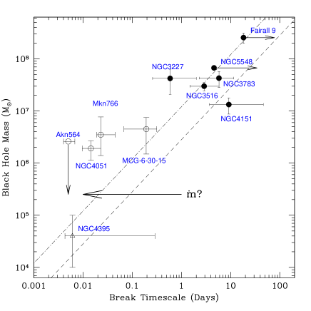
Figure 14: Black hole mass vs. PSD Break Timescale. Broad line Seyfert galaxies are shown as filled circles, narrow line Seyfert galaxies are shown as open circles and NGC4395 is shown as an open triangle. The dashed line to the right represents linear scaling of break timescale with mass from Cyg X-1 in its low state. The dot-dash line, on the left, represents linear scaling of break timescale with mass from Cyg X-1 in its high state. NGC4395 is plotted as an open triangle (see text). The arrow labelled with $\dot{m}$ indicates the way in which the relationship of break timescale vs. mass might move with increasing accretion rate.

References

- Akritas & Bershady (1996) Akritas M. G., Bershady M. A., 1996, ApJ, 470, 706
- Boroson (2003) Boroson T. A., 2003, ApJ, 585, 647
- Botte et al. (2005) Botte V., Ciroi S., di Mille F., Rafanelli P., Romano A., 2005, MNRAS, 356, 789
- Botte et al. (2004) Botte V., Ciroi S., Rafanelli P., Di Mille F., 2004, AJ, 127, 3168
- Brinkmann et al. (2000) Brinkmann W., Laurent-Muehleisen S. A., Voges W., Siebert J., Becker R. H., Brotherton M. S., White R. L., Gregg M. D., 2000, A&A, 356, 445
- Cui et al. (1997) Cui W., Heindl W. A., Rothschild R. E., Zhang S. N., Jahoda K., Focke W., 1997, ApJL, 474, L57
- Edelson & Nandra (1999) Edelson R., Nandra K., 1999, ApJ, 514, 682
- Elvis et al. (1994) Elvis M., Matsuoka M., Siemiginowska A., Fiore F., Mihara T., Brinkmann W., 1994, ApJL, 436, L55
- Elvis et al. (1989) Elvis M., Wilkes B. J., Lockman F. J., 1989, AJ, 97, 777
- Fender (2001) Fender R. P., 2001, in Black Holes in Binaries and Galactic Nuclei, p. 193
- Fender (2003) Fender R. P., 2003, Jets from X-ray binaries. Cambridge University Press, eds. W.H.G.Lewin and M. van der Klis (astro-ph/0303339)
- Ferrarese (2002) Ferrarese L., 2002, in Current high-energy emission around black holes, eds Lee, C.H and Chang, H.Y., Singapore, World Scientific, p. 3
- Ferrarese & Merritt (2000) Ferrarese L., Merritt D., 2000, ApJL, 539, L9
- Ferrarese et al. (2001) Ferrarese L., Pogge R. W., Peterson B. M., Merritt D., Wandel A., Joseph C. L., 2001, ApJL, 555, L79
- Filippenko & Ho (2003) Filippenko A. V., Ho L. C., 2003, ApJL, 588, L13
- Gallo et al. (2003) Gallo E., Fender R. P., Pooley G. G., 2003, MNRAS, 344, 60
- Greene et al. (2004) Greene J. E., Ho L. C., Barth A. J., 2004, in ”The Interplay among Black Holes, Stars and ISM in Galactic Nuclei”. Proceedings of IAU Symposium 222, astro-ph/0406047
- Herrero et al. (1995) Herrero A., Kudritzki R. P., Gabler R., Vilchez J. M., Gabler A., 1995, A&A, 297, 556
- Kaspi et al. (2000) Kaspi S., Smith P. S., Netzer H., Maoz D., Jannuzi B. T., Giveon U., 2000, ApJ, 533, 631
- Kraemer et al. (1999) Kraemer S. B., Ho L. C., Crenshaw D. M., Shields J. C., Filippenko A. V., 1999, ApJ, 520, 564
- Lee et al. (2000) Lee J. C., Fabian A. C., Reynolds C. S., Brandt W. N., Iwasawa K., 2000, MNRAS, 318, 857
- Maccarone (2003) Maccarone T. J., 2003, A&A, 409, 697
- Magorrian et al. (1998) Magorrian J. et al., 1998, AJ, 115, 2285
- Markowitz et al. (2003) Markowitz A. et al., 2003, ApJ, 593, 96
- McClintock & Remillard (2003) McClintock J. E., Remillard R. A., 2003, Compact Stellar X-ray Sources. Cambridge University Press, eds. W.H.G.Lewin and M. van der Klis (astro-ph/0306213)
- McHardy et al. (1981) McHardy I. M., Lawrence A., Pye J. P., Pounds K. A., 1981, MNRAS, 197, 893
- Merloni et al. (2003) Merloni A., Heinz S., di Matteo T., 2003, MNRAS, 345, 1057
- Merritt & Ferrarese (2001) Merritt D., Ferrarese L., 2001, ApJ, 547, 140
- Morales & Fabian (2002) Morales R., Fabian A. C., 2002, MNRAS, 329, 209
- McHardy (1988) McHardy I. M., 1988, Memorie della Societa Astronomica Italiana, 59, 239
- McHardy et al. (1998) McHardy I. M., Papadakis I. E., Uttley P., 1998, in The Active X-ray Sky: Results from BeppoSAX and RXTE, p. 509
- McHardy et al. (2004) McHardy I. M., Papadakis I. E., Uttley P., Page M. J., Mason K. O., 2004, MNRAS, 348, 783
- Nowak & Chiang (2000) Nowak M. A., Chiang J., 2000, ApJL, 531, L13
- Nowak et al. (1999) Nowak M. A., Vaughan B. A., Wilms J., Dove J. B., Begelman M. C., 1999, ApJ, 510, 874
- Padovani & Rafanelli (1988) Padovani P., Rafanelli P., 1988, A&A, 205, 53
- Peterson (2001) Peterson B. M., 2001, in ASP Conf. Ser. 224: Probing the Physics of Active Galactic Nuclei, p. 1
- Peterson et al. (2004) Peterson B. M. et al., 2004, ApJ, 613, 682
- Pineda et al. (1980) Pineda F. J., Delvaille J. P., Schnopper H. W., Grindlay J. E., 1980, ApJ, 237, 414
- Reynolds (2000) Reynolds C. S., 2000, ApJ, 533, 811
- Reynolds et al. (1997) Reynolds C. S., Ward M. J., Fabian A. C., Celotti A., 1997, MNRAS, 291, 403
- Shemmer et al. (2003) Shemmer O., Uttley P., Netzer H., McHardy I. M., 2003, MNRAS, 343, 1341
- Tanaka et al. (1995) Tanaka Y. et al., 1995, Nat, 375, 659
- Tremaine et al. (2002) Tremaine S. et al., 2002, ApJ, 574, 740
- Ulvestad & Wilson (1984) Ulvestad J. S., Wilson A. S., 1984, ApJ, 285, 439
- Uttley et al. (2002) Uttley P., McHardy I. M., Papadakis I. E., 2002, MNRAS, 332, 231
- van Groningen (1993) van Groningen E., 1993, A&A, 272, 25
- Vaughan et al. (2003) Vaughan S., Fabian A. C., Nandra K., 2003, MNRAS, 339, 1237
- Vaughan et al. (2005) Vaughan S., Iwasawa K., Fabian A. C., Hayashida K., 2005, MNRAS, 356, 524
- Vestergaard (2002) Vestergaard M., 2002, ApJ, 571, 733
- Wandel (1999) Wandel A., 1999, ApJL, 519, L39
- Wandel (2002) Wandel A., 2002, ApJ, 565, 762
- Wandel et al. (1999) Wandel A., Peterson B. M., Malkan M. A., 1999, ApJ, 526, 579
Acknowledgments
This work was supported by grant PPA/G/S/1999/00102 to IMcH from the UK Particle Physics and Astronomy Research Council (PPARC). IMcH also acknowledges the support of a PPARC Senior Research Fellowship. We thank Raylee Stathakis and the Service Programme of the Anglo Australian Telescope for carrying out the observations very efficiently. We thank Brad Peterson, Mike Merrifield and Andy Newsam for useful discussions.