The uBVI Photometric System. I. Motivation, Implementation, and Calibration

Abstract

This paper describes the design principles for a CCD-based photometric system that is highly optimized for ground-based measurement of the size of the Balmer jump in stellar energy distributions. It is shown that, among ultraviolet filters in common use, the Thuan-Gunn $u$ filter is the most efficient for this purpose. This filter is combined with the standard Johnson-Kron-Cousins $B$, $V$, and $I$ bandpasses to constitute the uBVI photometric system.

Model stellar atmospheres are used to calibrate color-color diagrams for the uBVI system in terms of the fundamental stellar parameters of effective temperature, surface gravity, and metallicity. The $u-B$ index is very sensitive to $\log g$, but also to ${\rm[Fe/H]}$. It is shown that an analog of the Strömgren $c_{1}$ index, defined as $(u-B)-(B-V)$, is much less metallicity dependent, but still sensitive to $\log g$. The effect of interstellar reddening on $u-B$ is determined through synthetic photometric calculations, and practical advice is given on dealing with flat fields, atmospheric extinction, the red leak in the $u$ filter, and photometric reductions.

The uBVI system offers a wide range of applicability in detecting stars of high luminosity in both young (yellow supergiants) and old (post-AGB stars) populations, using stars of both types as standard candles to measure extragalactic distances with high efficiency, and in exploring the horizontal branch in globular clusters. In many stellar applications, it can profitably replace the classical uBVI system.

Paper II in this series will present a network of well-calibrated standard stars for the uBVI system.

1 Introduction and Motivation

Stars of high intrinsic brightness are essential in a variety of astronomical applications, including their use as standard candles for measuring extragalactic distances, and as luminous tracers of stellar populations in external galaxies. In the future, such objects will serve as dynamical and chemical probes, through measurements of radial velocities and determinations of chemical abundances with spectrographs on large telescopes, and through space-based microarcsecond astrometry.

The visually brightest non-transient stars are Population I supergiants of A, F, and early G spectral types, hereafter called “yellow supergiants.” The rarest and most luminous of these stars attain visual absolute magnitudes as bright as $M_{V}\simeq-10$ (Humphreys 1983).

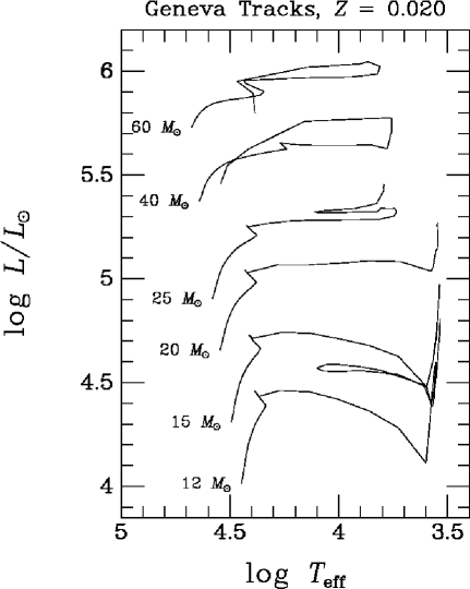
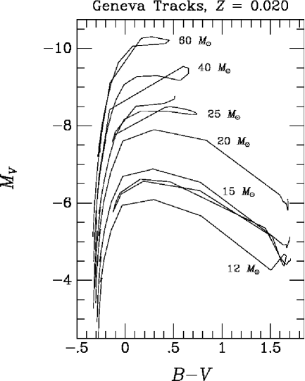
Figure 1: Left: Theoretical evolutionary tracks from the Geneva group (Meynet et al. 1994) in the standard theoretical coordinates, for stars of initial masses of 12–60 $M_{\odot}$. Right: Same tracks transformed to observational coordinates of absolute visual magnitude vs. $B-V$ color. This plot shows that yellow supergiants, with $B-V$ colors of about 0 to 0.5, are the visually brightest non-transient stars in galaxies, because of the behavior of the bolometric correction.

Yellow supergiants are the optically brightest stars because of the behavior of the bolometric correction, which is smallest at these spectral types but becomes quite large for blue and red supergiants. Fig. 1 illustrates this point. On the left are plotted evolutionary tracks for massive stars (Meynet et al. 1994), in the usual theoretical coordinates of $\log L/L_{\odot}$ vs. $\log T_{\rm eff}$. The plotted tracks are for solar metallicity ($Z=0.02$ by mass), and the models include mass loss. Each track is labelled with the star’s initial main-sequence mass. Following an initial rise off the main sequence, the stars evolve to cooler effective temperatures at roughly constant luminosity (with the more massive stars eventually turning back toward higher temperatures near the ends of their lives, and the less massive rising to very high luminosities as red supergiants).

On the right side of Fig. 1, these tracks have been converted to the observational quantities $M_{V}$ vs. $B-V$, using the formulae of Flower (1996). Now we see the dramatic fashion in which the observational tracks peak in brightness around types A and F (i.e., between $B-V\simeq 0$ and 0.5). The sharp peaking is due to the strong dependence of the bolometric correction upon $T_{\rm eff}$, which overwhelms the evolutionary variations in bolometric luminosity.

Likewise, the brightest stars of Population II are of spectral types A and F, but in this case they are low-mass post-asymptotic-giant-branch (PAGB) stars evolving off the tip of the AGB and passing through these spectral types on their way to the top of the white-dwarf cooling sequence. PAGB stars of these spectral types show great promise as Population II standard candles and as luminous tracers of old populations (Bond 1997; Alves, Bond, & Onken 2001).

In addition to their high optical luminosities, yellow supergiants and PAGB stars have the advantage of being easily detected through multicolor photometry. The reason is that, because of their very low surface gravities, their spectral energy distributions show extremely large Balmer discontinuities in the optical UV region. No other stellar objects have such large Balmer jumps, giving these stars a unique photometric signature that can be detected at low spectral resolution even at faint apparent magnitudes. Moreover, this signature can be detected in a single observation, unlike the time-series photometry needed to detect the subset of cooler and fainter yellow supergiants that are Cepheid variables.

The problem, however, is that historically there has not been a widely used photometric system that is fully optimized for the detection of faint stars with large Balmer jumps. The classical Johnson-Kron-Cousins $UBVRI$ system has been in use for nearly five decades, and extensive calibrations and networks of standard stars have been established through the heroic work of Landolt (1992) and many others. However, the $U$ filter of this system straddles the Balmer jump, and is thus far from optimum for measuring its size. (In fact, it is highly undesirable to straddle the jump, since when the size of the discontinuity increases due to lowering of the surface gravity, much of the extra absorbed flux is redistributed to wavelengths just longward of the jump.) By contrast, the $u$ filter of the $uvby$ system (Strömgren 1963) was specifically optimized to measure the Balmer jump by placing all of its transmission below $\sim$3650 Å; however, all four filters of this system have intermediate-width bandpasses, making the throughput undesirably low for efficient observations of faint stars in external galaxies. The intermediate-band $uvgr$ system introduced by Thuan & Gunn (1976) has the advantage of a $u$ filter lying almost entirely below the Balmer jump, but did not, at the time the work reported here was planned, have the wide usage and extensive calibration work of the $UBVRI$ and Strömgren systems for stellar photometry, especially in the southern hemisphere. The Thuan-Gunn system was modified to the wide-band $u^{\prime}g^{\prime}r^{\prime}i^{\prime}z^{\prime}$ filters for the Sloan Digital Sky Survey (Fukugita et al. 1996), but unfortunately (in the present context), in order to increase its throughput for work on faint extragalactic objects, the designers of this system adopted a $u^{\prime}$ filter with significant transmission above the Balmer discontinuity.

The purpose of the present paper is to describe a new CCD-based “uBVI” photometric system, which is highly optimized for detection of faint stars with large Balmer jumps, has high throughput for all four filters, and whose $BVI$ filters can be readily calibrated against the large body of existing stellar photometry that has accumulated over the past decades. Because of the wide use of the $UBVRI$ system for stellar work, including its extensive use for measurements of extragalactic standard candles, and its broad bandpasses, the writer quickly decided that, above the Balmer jump, one should simply adopt the standard $B$, $V$, and $I$ filters of the Johnson-Kron-Cousins system. The $I$ band was included because of its low sensitivity to interstellar extinction, and because $V-I$ provides a color index less sensitive to metallicity than $B-V$; moreover, the $I$ measurement provides an elegant means for dealing with the red leak of the chosen $u$ filter (see below). (For the sake of efficiency, it was felt that the $R$ filter would not provide sufficient additional information to justify its addition to the system.)

The following sections describe the selection of a UV filter to be added to $B$, $V$, and $I$; the calibration of the uBVI system based on model stellar atmospheres; determination of the interstellar extinction coefficients; and a discussion of some practical considerations in implementing this new photometric system. Paper II in this series (Siegel & Bond 2005) will describe our establishment of a network of equatorial standard stars for our uBVI system.

2 Selection of an Optimal UV filter

What is the optimum choice for a UV filter to measure the size of the Balmer jump? A narrow-bandpass filter lying entirely below the jump would have high sensitivity to the size of the discontinuity, but low observing efficiency. At the other extreme, a wide filter extending somewhat above the jump would transmit more photons, but would be less sensitive to the size of the discontinuity, especially because of the flux-redistribution effect described above. In typical applications, about 3/4 of the total observing time goes into the $u$-band exposures, so it is crucial to choose the most efficient filter if one plans to observe faint stars.

To make this efficiency assessment, I calculated a “figure of merit” for measuring the Balmer jump as follows. I consider an idealized experiment in which two solar-metallicity stars of the same apparent angular radius, both having $T_{\rm eff}=7000$ K (near the effective temperature at which the size of the jump is largest), are observed separately, one of surface gravity $\log g=4.5$ (main-sequence star) and the other with $\log g=1.0$ (typical of a Population I yellow supergiant or Population II PAGB star). Both stars are to be observed through the $u$ and $B$ filters, and the change in the instrumental $u-B$ color index is the measure of the change in the Balmer jump. The figure of merit then becomes the total exposure time (summed over the $u$ and $B$ observations of both stars) needed to measure the change in $u-B$ color index, $\Delta(u-B)$, to a given accuracy, say 1% of $\Delta(u-B)$. The optimum observing procedure would be to spread the error budget evenly over all 4 exposures, i.e., detect the same number of photons in each of the 4 exposures. In this idealization, I neglect such factors as sky background, and simply take the measurement errors to be proportional to the inverse square root of the number of detected photons.

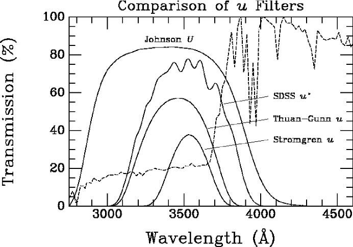
Figure 2: Comparison of the transmission curves (solid lines) for four candidate UV filters. Sources for the curves are given in the notes to Table 1. Note that these curves do not include the atmospheric transmission function, which will truncate the curves on the short-wavelength side, nor any instrumental or detector throughput factors. The dashed line plots the flux curve of a model atmosphere with $(T_{\rm eff},\log g,{\rm[Fe/H]})=(7000,1,0)$ in order to show the location of the Balmer jump. As discussed in the text and shown in Table 1, the Thuan-Gunn $u$ filter offers the best combination of sensitivity to the Balmer jump plus high throughput.

Calculations were made using the computational technique and model stellar atmospheres described in detail below, assuming unreddened stars and an airmass of 1.2. The detector sensitivity of the Cerro Tololo 0.9-m CCD camera, also described below, was adopted. The actual Johnson $B$ filter used in this camera was assumed, and four different candidate UV filters were considered: Thuan-Gunn $u$, Strömgren $u$, SDSS $u^{\prime}$, and Johnson $U$. Figure 2 plots the transmission curves of these four filters. In order to show the location of the Balmer jump, the flux distribution of a model atmosphere with $T_{\rm eff}=7000$ K, $\log g=1$, and ${\rm[Fe/H]}=0$, taken from Lejeune, Cuisinier, & Buser (1997, hereafter LCB97), is also plotted. Results of the calculations are presented in Table 1. The notes at the end of Table 1 give the sources for the filter transmission curves used in the calculations.

The table shows that the Thuan-Gunn $u$ filter is the best choice by a considerable margin. Although Strömgren $u$ is more sensitive to surface gravity [that is, it has the largest $\Delta(u-B)$, because it transmits essentially no flux above 3650 Å], it is not the most efficient, because of its relatively low throughput. The $u^{\prime}$ and $U$ filters have higher throughput, but lower sensitivity to $\log g$ because they have significant transmission above the Balmer jump, and are thus likewise sub-optimal.

I therefore chose to adopt the Thuan-Gunn $u$ as the ultraviolet filter. Details of the Thuan-Gunn $u$ filter (hereafter called simply “$u$” when there is no ambiguity), including the recipe for constructing it, and a measured transmission curve, are given in Appendix A.

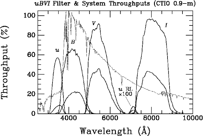
Figure 3: Filter transmission curves for the uBVI filters (upper solid lines) and system throughput curves for the Cerro Tololo 0.9-m telescope/CCD camera combined with the atmospheric transmission at airmass 1.2 (lower solid lines). The red-leak transmission and system throughput of the Thuan-Gunn $u$ filter is also plotted, scaled up by a factor of 100. Also plotted is the flux distribution for a model atmosphere with $(T_{\rm eff},\log g,{\rm[Fe/H]})=(7000,1,0)$ (light dashed curve), taken from Lejeune et al. 1997.

Figure 3 plots the transmission curves for the uBVI filters alone, and the total system throughput curves, for the Cerro Tololo Interamerican Observatory (CTIO) 0.9-m telescope, filters, and CCD camera, viewing through an airmass of 1.2 (calculated as described below). Also shown, again in this figure, is the LCB97 flux distribution for a low-gravity F star ($T_{\rm eff}=7000$ K, $\log g=1$, ${\rm[Fe/H]}=0$).

Table 2 summarizes some basic properties of the four filters of this new uBVI system. The final column lists references for the nominal effective wavelengths and full widths at half maximum (FWHM) for the filters. As noted in the table and discussed below, the zero points for the uBVI magnitudes will be set such that Vega will have magnitude zero in $BVI$, but magnitude 1.00 at $u$.

3 Calibration of Stellar Atmospheric Parameters

3.1 Computational Method

In this section I present calculations of the dependence of colors in the uBVI system upon the fundamental stellar parameters of effective temperature, surface gravity, and metallicity.

Stellar magnitudes, $m$, are defined with the usual equation

$$m=-2.5\log n_{\rm phot}+{\rm const}\,,$$ (1)

where $n_{\rm phot}$ is the number of photons detected from a star using a given filter, CCD camera, and telescope system. The number of detected photons is given by the following equation:

$$n_{\rm phot}\propto\int_{0}^{\infty}\lambda F_{\lambda}(T_{\rm eff},\log g,{\rm[Fe/H]};\lambda)\,I[E(B-V),\lambda]\,A(\lambda)^{X}\,r(\lambda)^{2}\,T(\lambda)\,Q(\lambda)\,d\lambda\,.$$ (2)

The terms in eq. 2 have been arranged in order from the star to the detector, and have the following meanings:

1. $\lambda F_{\lambda}(T_{\rm eff},\log g,{\rm[Fe/H]};\lambda)$ is the photon flux from a star of a given effective temperature, surface gravity, and metallicity. $F_{\lambda}$ is multiplied by the wavelength $\lambda$ in eq. 2 in order to convert energy flux to photon flux, since the CCD detector signal is proportional to the number of photons. Throughout this paper I have obtained stellar fluxes from the library of “corrected” synthetic stellar spectra presented by LCB97. LCB97 actually tabulate the Eddington flux $H_{\nu}$, which, as they note, should be converted to $F_{\lambda}$ using $F_{\lambda}=0.4H_{\nu}c/\lambda^{2}$.

2. $I[E(B-V),\lambda]$ is the attenuation due to interstellar extinction. I have used the analytic formulae of Cardelli, Clayton, & Mathis (1989) with $R_{V}$ set to 3.1.

3. $A(\lambda)$ is the Earth’s atmospheric transmission as a function of wavelength at an airmass $X=1$. This function was set equal to the mean of the atmospheric extinction curves measured on 38 nights of spectrophotometry at CTIO between 1988 and 1994 by Hamuy et al. (1994), kindly provided to the writer in tabular form by Hamuy (1999). I make the assumption that the same curve can be used to simulate observations made at Kitt Peak National Observatory (KPNO). Hamuy tabulates extinction coefficients in magnitudes per airmass, $k(\lambda)$, which are converted to atmospheric transmission using $A(\lambda)=10^{-k(\lambda)/2.5}$. At airmasses other than 1, $A(\lambda)$ must be raised to the power $X$.

4. $r(\lambda)$ is the attenuation due to reflection from an aluminum surface, taken from Allen (1973a). It is squared in eq. 2 because there are two such reflections in the Cassegrain telescope systems used in this work.

5. $T(\lambda)$ is the transmission of the filter. For the work described here and in Paper II, virtually all of the observations were made at just two telescopes, the 0.9-m reflectors at CTIO and KPNO, using the same $u$-band filter. Thus, detailed simulations of the $u$-band magnitudes have been carried out for these specific telescope and camera systems. The transmission data for the $u$ filter are given in Appendix A of the present paper.

6. Finally, $Q(\lambda)$ is the quantum efficiency of the CCD detector. Tables for this were kindly provided by Walker (2000) for the Tek3 CCD used on the CTIO 0.9-m telescope, and by Jacoby (1999) for the T2KA CCD used at the KPNO 0.9-m.

The calculations for the $B$ filter were handled slightly differently from the above, since I wanted to simulate $B$ magnitudes that have been transformed to the standard system (rather than instrumental magnitudes, which were calculated for the $u$ band as just described). Therefore, for $B$ I adopted the response function tabulated by Azusienis & Straizys (1969), choosing their outside-atmosphere tabulation. (This table has also been re-published by Buser & Kurucz 1978, and widely used in simulations of the $UBVRI$ system.) Since Azusienis & Straizys determined the full system response for the standard $B$ filter, I equated $r(\lambda)^{2}\,T(\lambda)\,Q(\lambda)$ to their values in my eq. 2.

In general, I did not re-calculate $B-V$ and $V-I$ colors, since these have already been tabulated by LCB97 for their model atmospheres. However, for the red-leak simulations in §5.3, I did need to calculate instrumental magnitudes in the $I$ band. For these computations, I used filter transmission curves measured by NOAO staff members; for the CTIO 0.9-m system, the functions were obtained from the website http://www.ctio.noao.edu/instruments/filters/, and for the KPNO 0.9-m from ftp://ftp.noao.edu/kpno/filters/4Inch_List.html.

3.2 Stellar Atmospheric Calibrations

In order to simulate the behavior of the uBVI system, in particular its sensitivity to the basic stellar parameters, I have performed numerical integrations using eq. 2 for model-atmosphere fluxes taken from LCB97. For the $B-V$ and $V-I$ colors, I simply adopted those tabulated by LCB97. For $u-B$, as described above, I calculated instrumental $u$ magnitudes for the CTIO 0.9-m telescope with the Tek3 CCD camera, combined with $B$ magnitudes calculated for the standard $B$ response function. The calculations were done for magnitudes outside the atmosphere (i.e., I set $X=0$ in eq. 2), and for unreddened stars. Magnitudes in the $u$ band were calculated for the main ultraviolet bandpass alone, and excluded the contribution from the filter’s red leak (see below).

The constants in eq. 1 were set such that the $u-B$ color of the LCB97 model atmosphere with $T_{\rm eff}=9500$ K, $\log g=4.0$, and ${\rm[Fe/H]}=-0.5$, which are very close to the atmospheric parameters of Vega (Castelli & Kurucz 1994), is $u-B=1.0$. The $B-V$ and $V-I$ colors of this model, tabulated by LCB97, are of course essentially 0.0 (actually, they are $-0.012$ and $-0.021$, respectively). I have thus followed the precepts of Strömgren (1963), who set the $u-b$ color of Vega and other A0 V stars to 1.0 in the $uvby$ system. Given the considerable drop in flux below the Balmer jump, this is a more realistic choice than setting $u-B=0.0$, as was done, for example, in the classical $UBV$ system (Johnson & Morgan 1953), or in other “Vega-mag” photometric systems.

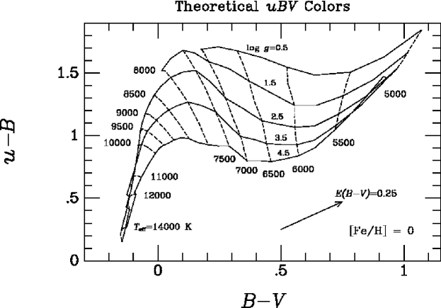
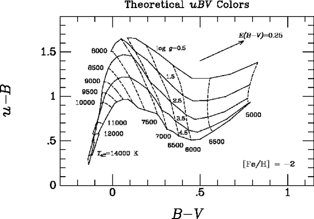
Figure 4: $u-B$ vs. $B-V$ color-color relations for stars of solar metallicity (a, top) and 1% of solar metallicity (b, bottom). Dashed lines are lines of constant effective temperature, and solid lines are lines of constant surface gravity, as labelled. Slopes of reddening vectors are indicated. Note that $u-B$ is very sensitive to $\log g$ for stars up to $T_{\rm eff}\simeq 10,000$ K. $u-B$ and $B-V$ are, however, also sensitive to metallicity.

Figure 4a shows the $u-B$ vs. $B-V$ color-color diagram for stars of solar metallicity, effective temperatures of 5,000 to 14,000 K, and surface gravities of $\log g=0.5$ to 4.5. (Note that in this and similar diagrams, I plot $u-B$ increasing upwards, rather than downwards as is the convention in the $UBV$ system; this is done in order to have high-luminosity stars lie near the top of the diagram, as is the convention in similar plots in the Strömgren system.) Figure 4b is the same diagram, but for stars of ${\rm[Fe/H]}=-2$. Lines of constant effective temperature (dashed) and of constant surface gravity (solid) are drawn and labelled. These figures show the high sensitivity of the $u-B$ color index to gravity for stars of 5,000 K up to about 10,000 K. As is well known, above about 10,000 K, the Balmer jump (and hence the $u-B$ color index) is not highly sensitive to $\log g$, but remains sensitive to $T_{\rm eff}$. Unfortunately, however, both $u-B$ and $B-V$ are quite sensitive to metallicity, as a comparison of Figures 4a and 4b shows, since both indices become significantly bluer as ${\rm[Fe/H]}$ is reduced.

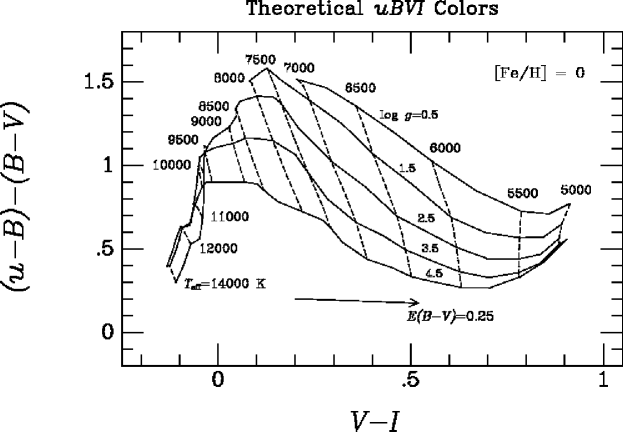
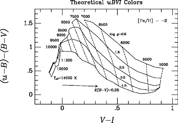
Figure 5: $(u-B)-(B-V)$ vs. $V-I$ color-color relations for stars of solar metallicity (a, top) and 1% of solar metallicity (b, bottom). Labelling of $T_{\rm eff}$ and $\log g$ is as in Figures 4a-4b, and slopes of reddening vectors are indicated. The $(u-B)-(B-V)$ color difference, which is an analog of the $c_{1}$ index in the Strömgren $uvby$ system, has the advantage of lower sensitivity to metallicity and reddening than the $u-B$ index, while retaining high sensitivity to surface gravity. $V-I$ is also considerably less sensitive to metallicity than $B-V$.

The metallicity dependence can be mitigated to a considerable extent by adopting a color difference analogous to the Strömgren $c_{1}$ index, which he defined as $c_{1}=(u-v)-(v-b)$ (where $u$ here is, of course, Strömgren’s $u$). Such an index retains a high sensitivity to gravity, but is less sensitive to metallicity (and also to interstellar reddening). For the uBVI system, I adopt the color difference $(u-B)-(B-V)$, which I plot against $V-I$ in the color-color diagrams in Figures 5a and 5b. In these figures, we see that $V-I$ is much less sensitive to metallicity, as is $(u-B)-(B-V)$ except for stars below $\sim$6,000 K, where some metallicity dependence remains. As anticipated, the $(u-B)-(B-V)$ is very sensitive to $\log g$. (It would, if desired, be possible to define more complicated color-difference formulae with $V-I$ color terms, with even less sensitivity to metallicity and/or reddening, similar to the reddening-free $[c_{1}]$ index used in the Strömgren system, e.g., Strömgren 1966.)

Detailed tables of the color grids are available upon request from the author.

3.3 Zero-Age Main-Sequence Relation

It is useful for many purposes to have color-color relations available for the zero-age main sequence (ZAMS). I have calculated such relations for $u-B$ vs. $B-V$ and $(u-B)-(B-V)$ vs. $V-I$, both at solar metallicity. The calculations were done by interpolation in $T_{\rm eff}$ and $\log g$ in the color-color grids, using the table of main-sequence surface gravities vs. spectral type given by Allen (1973b) and the table of effective temperatures vs. spectral type given by Drilling & Landolt (2000).

The ZAMS relations are given in Table 3.

4 Interstellar Extinction

The dependence of the $u-B$ and $(u-B)-(B-V)$ color excesses upon interstellar extinction was calculated using eq. 2 and varying the $B-V$ color excess, $E(B-V)$. As noted above, all of the calculations are based on the reddening formula of Cardelli et al. (1989), with $R_{V}=3.1$. Because of the finite width of the $u$ bandpass, the color-excess ratios depend weakly on the stellar parameters, and are also slightly non-linear functions of $B-V$. However, for most purposes, it will be adequate to adopt the ratios for a lightly reddened, “typical” star. For a star of ($T_{\rm eff},\log g,{\rm[Fe/H]})=(7000,2.5,0)$, i.e., a star lying near the middle of the color-color grid of Figure 4a, and small amounts of reddening, the calculations show that the color-excess ratios are given by:

$$E(u-B) = 0.89\,E(B-V)\,,$$ (3)

$$E[(u-B)-(B-V)] = -0.11\,E(B-V)\,.$$ (4)

For completeness, I note that the following relation has been given for the color excess in $$V-I$$ by Dean, Warren, & Cousins (1978):

$$E(V-I) = 1.25[1+0.06(B-V)_{0}+0.014E(B-V)]\,E(B-V)\,.$$ (5)

The slopes of these reddening vectors are plotted in Figures 4a-b and 5a-b.

5 Practical Considerations

Other astronomers who may wish to implement the uBVI system for their own programs should take into account the following considerations when planning and obtaining their observations and in reducing their data.

5.1 Flat Fields

It is usually satisfactory to perform flat-fielding of the CCD frames in $B$, $V$, and $I$ by exposing on a uniformly illuminated white surface placed in front of the telescope (“dome flats”). However, in most dome-flat setups, the illumination of the white surface is from incandescent lamps with a low color temperature. These would be completely unsatisfactory for the $u$ filter, because most of the signal would be transmitted through the filter’s red leak. Hence it is essential that the $u$-band flats be obtained on the clear sky at twilight. These flats should generally be taken a few minutes after sunset and/or a few minutes before sunrise, while the twilit sky is bright enough. With wide-field imaging systems, care should be taken to point the telescope so as to avoid brightness gradients in the twilight illumination across the field (see, for example, Chromey & Hasselbacher 1996).

5.2 Atmospheric Extinction

Since the effective wavelength of the $u$ bandpass changes significantly with stellar color (redder effective wavelength for redder stars) and it changes with airmass (redder effective wavelength at higher airmass, due to the steep increase in extinction at shorter wavelengths), it is desirable to include both a color term and a non-linear airmass term in the extinction corrections.

Simulations of the extinction behavior were performed using numerical integrations based on eq. 2, varying both the stellar parameters and the airmass $X$. The system throughput of the CTIO 0.9-m camera and CCD was adopted, and the extinction coefficients were fitted to the following equation:

$$u_{\rm instr}(X)=u_{\rm out}+k_{1}X+k_{2}X^{2}\,,$$ (6)

where $u_{\rm instr}(X)$ is the instrumental $u$ magnitude measured at airmass $X$, $u_{\rm out}$ is the $u$ magnitude that would be measured outside the atmosphere, and $k_{1}$ and $k_{2}$ are the linear and quadratic extinction coefficients. Least-squares fits to the simulated magnitudes show that $k_{1}$ can be represented adequately as a linear function of $B-V$ color,

$$k_{1}=a+b(B-V)\,,$$ (7)

and that $k_{2}$ is essentially constant.

Eq. 6 therefore becomes

$$u_{\rm instr}(X)=u_{\rm out}+[a+b(B-V)]X+k_{2}X^{2}\,,$$ (8)

and the fit to the simulations yielded $a=0.615$, $b=-0.033$, and $k_{2}=-0.007$.

Extinction simulations were also run for the other three filters, and it was found (as is generally adopted in $BVI$ photometry) that there are no significant color or non-linear terms for the $V$ and $I$ filters, nor is there a significant non-linear term for the $B$ extinction. However, a $b$ color term of about $b=-0.03$ is appropriate for the $B$ filter.

In practical observing situations, the recommended procedure is always to observe a few standard fields at both low and high airmass during the night, and to solve by least squares for the $a$ coefficient (which is indeed observed to vary significantly from night to night). If there is a sufficient range of color among the standard stars, $b$ can also be solved for, or alternatively simply taken to be $-0.033$. However, in most actual situations, there will be insufficient observations to solve for $k_{2}$, and it is recommended that it simply be adopted as $k_{2}=-0.007$. The best practice is to observe the standard stars (apart from the extinction observations) and program stars over as small a range of airmass as possible, so as to lessen the impact of uncertainties in the extinction coefficients.

Note that most data-taking systems record the airmass at the start of the exposure, not at the photon-weighted effective midpoint; this correction is important in the $u$ band at high airmass and/or for long exposures, and the IRAF routine setairmass should be used to calculate the effective airmass.

5.3 Red Leak

As mentioned above, and shown in Figure 3, the $u$-filter glass combination chosen for the uBVI system has a significant red leak at about 7100 Å. Ideally, this leak should have been suppressed by adding another filter (such as liquid or crystal CuSO₄), or by applying a leak-blocking coating to the filter similar to that used for the SDSS $u^{\prime}$ filter (Fukugita et al. 1996). However, in the interests of economy, simplicity, and making the throughput of the $u$ filter as high as possible in the main bandpass, it was decided not to attempt to suppress the red leak.

Simulations of the contribution of the red leak to the total photon count in $u$ frames were calculated using eq. 2 for a range of stellar parameters and airmasses. Two observational approaches were considered: (1) calculate the red leak as a fraction of the total signal in the $u$ band as a function of stellar color and airmass, and (2) take advantage of the fact that the red leak lies at the short-wavelength edge of the $I$ bandpass, so that the red-leak signal in the $u$ band should be a simple function of the $I$-band signal, with a weak color term.

The simulations suggest that either approach is viable, but that the second one (basing the red-leak correction on the measured photon count in the $I$ band) has the advantage of no appreciable dependence on airmass. Least-squares fits to the simulations (for the CTIO 0.9-m system) yielded the following formulae:

$$\log({\rm RL}/u) = -2.662+2.019(B-V)-3.545(B-V)^{2}$$ (9)

$$+3.336(B-V)^{3}-0.9086(B-V)^{4}$$

$$+[0.2076-0.001157(B-V)-0.01902(B-V)^{2}](X-1.0)$$

$${\rm RL}/I = 0.0002268-0.0000680(B-V)$$ (10)

$$+0.0000536(B-V)^{2}-0.0000300(B-V)^{3}\,,$$

where RL is the contribution to the $u$ counts due to the red leak, $u$ is the total detected photon counts (main band plus red leak), $B-V$ is the color of the star on the standard system, $I$ is the photon count in the $I$ band, and $X$ is airmass. All photon counts are per unit time. It should be noted that the corrections of eqs. 9 and 10 are to be made to the observed inside-atmosphere $u$ counts before the atmospheric extinction is removed. Similar equations were calculated for the KPNO 0.9-m system (see Paper II).

Eq. 9 shows that, near the zenith, the red leak is predicted to contribute about 1% of the total $u$ signal for stars with $B-V=0.8$, 10% of the signal at $B-V=1.47$, and 30% at $B-V=1.85$. Thus, since the uBVI system is intended primarily for the study of stars of spectral types A through early G, the red leak can usually simply be neglected. For the most accurate work, the correction should be made, using eq. 10 if $I$-band observations have been made, or eq. 9, if a system similar to that of the CTIO 0.9-m telescope is used. Alternatively, in many cases it will be most practical (especially if the necessary laboratory measurements of the camera and filter system are not available) to reduce the $u$-band photometry to the system defined by the standard stars listed in Paper II, without making any explicit red-leak corrections. If the reddest stars are excluded, any remaining adjustments for red leak will be absorbed in linear and quadratic terms in $B-V$ in the transformation equation. In the standard stars listed in Paper II, we have excluded all stars with $B-V>1.45$, and have found that such transformations reproduce the red-leak-corrected $u$ magnitudes adequately.

5.4 Reduction Procedures

In summary, it is recommended that uBVI photometric observations be reduced as follows:

1. Reduce the $BVI$ observations to the system defined by the Landolt (1992) standard stars, using conventional techniques to remove atmospheric extinction and then transform the instrumental magnitudes to the standard system.

2. If desired and if possible, correct each $u$ observation inside the atmosphere for red leak, as described above (eq. 9 or 10).

3. Then, using standard fields observed at low and high airmass, solve for the $u$-band extinction coefficients in eq. 8 (adopting the values recommended above for $b$ and $k_{2}$).

4. After removing atmospheric extinction, fit the instrumental outside-atmosphere magnitudes of the standard stars, $u_{\rm out}$, to the standard values from Paper II, $u_{\rm std}$, using a conventional transformation equation of the form

$$u_{\rm out}=u_{\rm std}+c+d(B-V)+e(B-V)^{2}\,,$$ (11)

where $u$ is the standard magnitude, and $B-V$ is the color index on the standard system.

5. An alternative to the above procedure is to perform both the extinction correction and the transformation to the standard-star system through a single least-squares fit to an equation of the following form:

$$u_{\rm instr}=u_{\rm std}+[a+b(B-V)]X+k_{2}X^{2}+c+d(B-V)+e(B-V)^{2}\,.$$ (12)

In most practical cases, it will be adequate to set $k_{2}=0$.

6. Finally, using the above extinction and transformation equation(s), transform the program-star $u$ observations to the standard system.

6 Conclusion

I have described a CCD-based uBVI photometric system that is highly optimized for measurement of the Balmer jump in faint stars of spectral types A through early G. Since the size of the Balmer jump is very sensitive to stellar surface gravity in such stars, the uBVI system should be useful in applications involving determination of stellar luminosities and measurement of extragalactic distances through high-luminosity standard candles of Populations I and II. This system should also find application in the study of phenomena on the horizontal branch in globular clusters (e.g., Grundahl et al. 1999), or indeed in a variety of settings involving stars too faint for efficient observations in the Strömgren $uvby$ system.

Future papers in this series will report results of extensive uBVI observations of Galactic globular clusters and the halos and disks of nearby galaxies.

Appendix A Details of the Thuan-Gunn u Filter

Following the precepts of Thuan & Gunn (1976), the writer has had constructed several $u$ filters of various sizes. These filters are fabricated from Schott glasses as follows: 4 mm UG11 + 1 mm BG38. For comparison, the UG11 filter, but with different thicknesses, is also used for Strömgren $u$ (8 mm UG11 + 1 mm WG3) and SDSS $u^{\prime}$ (1 mm UG11 + 1 mm BG38).

All of the standard-star observations described in Paper II (Siegel & Bond 2005) were accomplished with a $4\times 4$ inch $u$ filter kindly constructed by Mr. Ed Carder of Kitt Peak National Observatory. Carder also kindly measured the transmission curve for this filter using the Lambda 9 spectrophotometer at KPNO. The data are presented in Table 4.

Table 1: Figures of Merit for Candidate UV Filters

Filter	$\Delta(u-B)$	Relative exposure time
Thuan-Gunn $u$	0.841	1.00
Strömgren $u$	0.889	2.01
SDSS $u^{\prime}$	0.488	1.36
Johnson $U$	0.380	1.44

Note. — Col. 1: Filter name. Sources of filter transmission curves are as follows. Thuan-Gunn $u$: Table 3 of this paper; SDSS $u^{\prime}$: Fukugita 2004; Strömgren $u$: ftp://ftp.noao.edu/kpno/filters/4indata/kp1538; Johnson $U$: Landolt 1992, Table 8; Johnson $B$: http://www.ctio.noao.edu/instruments/filters/; col. 2: Change in instrumental $u-B$ color index at airmass 1.2 for 7000 K stars when $\log g$ is changed from 4.5 to 1.0; col. 3: Relative exposure times required to measure $\Delta(u-B)$ to a given percentage error. See text for further explanation.

Table 2: Properties of uBVI Filters

Filter	Vega mag	$\lambda_{\rm eff}$ (Å)	FWHM (Å)	Reference
$u$	1.00	3530	1400	Thuan & Gunn 1976
$B$	0.00	4747	1409	Fukugita et al. 1996
$V$	0.00	5470	1826	Fukugita et al. 1996
$I$	0.00	8020	1543	Fukugita et al. 1996

Table 3: Zero-Age Main-Sequence Relation at ${\rm[Fe/H]}=0$

$T_{\rm eff}$ (K)	$\log g$	$B-V$	$u-B$	$V-I$	$(u-B)-(B-V)$
14000	4.04	$-$0.140	0.261	$-$0.130	0.401
13000	4.04	$-$0.124	0.378	$-$0.114	0.502
12500	4.04	$-$0.115	0.448	$-$0.106	0.563
12000	4.04	$-$0.105	0.528	$-$0.097	0.633
11500	4.04	$-$0.112	0.547	$-$0.074	0.659
11000	4.06	$-$0.087	0.680	$-$0.064	0.766
10500	4.10	$-$0.063	0.786	$-$0.055	0.850
10000	4.13	$-$0.034	0.896	$-$0.046	0.930
9750	4.14	$-$0.017	0.945	$-$0.038	0.962
9500	4.17	$-$0.002	0.969	$-$0.022	0.971
9250	4.19	0.018	0.988	0.006	0.972
9000	4.21	0.044	1.014	0.059	0.970
8750	4.24	0.073	1.037	0.089	0.970
8500	4.26	0.105	1.036	0.105	0.938
8250	4.28	0.142	1.019	0.139	0.872
8000	4.30	0.189	0.996	0.202	0.811
7750	4.31	0.235	0.968	0.259	0.736
7500	4.33	0.282	0.954	0.284	0.675
7250	4.34	0.319	0.895	0.318	0.575
7000	4.34	0.358	0.827	0.383	0.469
6750	4.34	0.408	0.825	0.447	0.417
6500	4.35	0.457	0.811	0.500	0.354
6250	4.37	0.513	0.827	0.564	0.314
6000	4.39	0.572	0.848	0.631	0.276
5750	4.44	0.639	0.907	0.705	0.268
5500	4.49	0.722	1.052	0.783	0.330
5250	4.49	0.812	1.231	0.844	0.419
5000	4.50	0.918	1.474	0.904	0.556

Table 4: Transmission Curve for Thuan-Gunn $u$ Filter

Wavelength (Å)	Transmission (%)	Wavelength (Å)	Transmission (%)
3000	11.000	6900	.000
3010	11.015	6910	.005
3020	11.050	6920	.005
3030	11.115	6930	.010
3040	11.240	6940	.015
3050	11.465	6950	.015
3060	11.850	6960	.020
3070	11.420	6970	.025
3080	12.225	6980	.025
3090	13.300	6990	.030
3100	14.675	7000	.035
3110	16.375	7010	.040
3120	18.280	7020	.045
3130	10.455	7030	.050
3140	12.770	7040	.055
3150	15.245	7050	.055
3160	17.745	7060	.060
3170	20.275	7070	.065
3180	22.830	7080	.065
3190	25.270	7090	.070
3200	27.705	7100	.075
3210	30.095	7110	.075
3220	32.360	7120	.075
3230	34.595	7130	.075
3240	36.670	7140	.075
3250	38.700	7150	.070
3260	40.610	7160	.070
3270	42.385	7170	.070
3280	44.125	7180	.065
3290	45.560	7190	.060
3300	47.065	7200	.055
3310	48.375	7210	.050
3320	49.610	7220	.045
3330	50.755	7230	.045
3340	51.785	7240	.040
3350	52.670	7250	.035
3360	53.425	7260	.030
3370	54.190	7270	.025
3380	54.770	7280	.025
3390	55.340	7290	.020
3400	55.730	7300	.015
3410	56.155	7310	.015
3420	56.420	7320	.015
3430	56.705	7330	.010
3440	56.810	7340	.010
3450	57.025	7350	.005
3460	56.965	7360	.005
3470	57.025	7370	.000
3480	56.920	7380	.000
3490	56.795	7390	.000
3500	56.565	7400	.000
3510	56.210
3520	55.840
3530	55.315
3540	54.800
3550	54.120
3560	53.270
3570	52.345
3580	51.300
3590	50.195
3600	48.910
3610	47.480
3620	45.990
3630	44.270
3640	42.455
3650	40.460
3660	38.305
3670	36.005
3680	33.675
3690	31.165
3700	28.555
3710	25.870
3720	23.165
3730	20.415
3740	17.715
3750	15.040
3760	12.565
3770	10.210
3780	18.080
3790	16.180
3800	14.570
3810	13.255
3820	12.235
3830	11.460
3840	11.905
3850	11.535
3860	11.290
3870	11.150
3880	11.065
3890	11.025
3900	11.005

References

- (1)
- (2) Allen, C. W. 1973a, Astrophysical Quantities (London: Athlone Press), 108
- (3) Allen, C. W. 1973b, Astrophysical Quantities (London: Athlone Press), 213
- (4) Alves, D. R., Bond, H. E., & Onken, C. 2001, AJ, 121, 318
- (5) Ažusienis, A., & Straižys, V. 1969, Soviet Astr., 13, 316
- (6) Bond, H. E. 1997, in The Extragalactic Distance Scale, ed. M. Livio, M. Donahue, & N. Panagia (Cambridge: Cambridge University Press), 224
- (7) Buser, R., & Kurucz, R. L. 1978, A&A, 70, 555
- (8) Cardelli, J. A., Clayton, G. C., & Mathis, J. S. 1989, ApJ, 345, 245
- (9) Castelli, F., & Kurucz, R. L. 1994, A&A, 281, 817
- (10) Chromey, F. R. & Hasselbacher, D. A. 1996, PASP, 108, 944
- (11) Dean, J. F., Warren, P. R., & Cousins, A. W. J. 1978, MNRAS, 183, 569
- (12) Drilling, J. S., & Landolt, A. U. 2000, in Allen’s Astrophysical Quantities (New York: AIP Press), ed. A. N. Cox, 381
- (13) Flower, P. J. 1996, ApJ, 469, 355
- (14) Fukugita, M. 2004, private communication
- (15) Fukugita, M., Ichikawa, T., Gunn, J. E., Doi, M., Shimasaku, K., & Schneider, D. P. 1996, AJ, 111, 1748
- (16) Grundahl, F., Catelan, M., Landsman, W. B., Stetson, P. B., & Andersen, M. I. 1999, ApJ, 524, 242
- (17) Hamuy, M. 1999, private communication
- (18) Hamuy, M., Suntzeff, N. B., Heathcote, S. R., Walker, A. R., Gigoux, P., & Phillips, M. M. 1994, PASP, 106, 566
- (19) Humphreys, R.M. 1983, ApJ, 269, 335
- (20) Jacoby, G. H. 1999, private communication
- (21) Johnson, H. L., & Morgan, W. W. 1953, ApJ, 117, 313
- (22) Kinman, T. D., Suntzeff, N. B., & Kraft, R. P. 1994, AJ, 108, 1722
- (23) Landolt, A. U. 1992, AJ, 104, 340
- (24) Lejeune, T., Cuisinier, F., & Buser, R. 1997, A&AS 125, 229 (LCB97)
- (25) Meynet, G., Maeder, A., Schaller, G., Schaerer, D., & Charbonnel, C. 1994, A&AS, 103, 97
- (26) Siegel, M. S., & Bond, H. E. 2005, submitted (Paper II)
- (27) Strömgren, B. 1963, in Basic Astronomical Data, ed. K. A. Strand (Chicago: University of Chicago Press), 123
- (28) Strömgren, B. 1966, ARA&A, 4, 433
- (29) Thuan, T. X., & Gunn, J. E. 1976, PASP, 88, 543
- (30) Walker, A. R. 2000, private communication