Soft X-ray and Ultraviolet Emission Relations in Optically Selected AGN Samples

Abstract

Using a sample of 228 optically selected Active Galactic Nuclei (AGNs) in the 0.01–6.3 redshift range with a high fraction of X-ray detections (81–86%), we study the relation between rest-frame UV and soft X-ray emission and its evolution with cosmic time. The majority of the AGNs in our sample (155 objects) have been selected from the Sloan Digital Sky Survey (SDSS) in an unbiased way, rendering the sample results representative of all SDSS AGNs. The addition of two heterogeneous samples of 36 high-redshift and 37 low-redshift AGNs further supports and extends our conclusions. We confirm that the X-ray emission from AGNs is correlated with their UV emission, and that the ratio of the monochromatic luminosity emitted at 2 keV compared to 2500 Å decreases with increasing luminosity ($\alpha_{\textrm{\scriptsize{ox}}}=-0.136l_{\textrm{\scriptsize{uv}}}+2.616$, where $l_{\textrm{\scriptsize{uv}}}$ is in $\log$ units), but does not change with cosmic time. These results apply to intrinsic AGN emission, as we correct or control for the effects of the host galaxy, UV/X-ray absorption, and any X-ray emission associated with radio emission in AGNs. We investigate a variety of systematic errors and can thereby state with confidence that (1) the $\alpha_{\textrm{\scriptsize{ox}}}$–$l_{\textrm{\scriptsize{uv}}}$ anti-correlation is real and not a result of accumulated systematic errors and (2) any $\alpha_{\textrm{\scriptsize{ox}}}$ dependence on redshift is negligible in comparison. We provide the best quantification of the $\alpha_{\textrm{\scriptsize{ox}}}$–$l_{\textrm{\scriptsize{uv}}}$ relation to date for normal radio-quiet AGNs; this should be of utility for researchers pursuing a variety of studies.

1. Introduction

Surveys for Active Galactic Nuclei (AGNs) were until recently most commonly conducted in the observed optical band (corresponding to the rest-frame UV for high-redshift AGNs); consequently, our understanding of the AGN population is biased toward properties inferred from AGN samples bright in the optical. Radio, infrared, and X-ray surveys have revealed more reddened and obscured AGNs, attesting to the presence of an optical bias. AGN surveys in non-optical bands still require optical or UV spectroscopy to confirm the presence of an active nucleus (except for bright, hard X-ray selected AGNs, or AGNs with large radio jets) and to determine the redshift. Historically, our understanding of the evolution of the luminous AGN population with cosmic time has been based largely on optically selected AGN samples; use of samples selected in other bands to further this understanding requires proper interpretation of the relations between emission in these bands and optical/UV emission for comparison. X-ray surveys are more penetrating and efficient in separating the host-galaxy contribution from the nuclear emission for sources with $L_{\textrm{\scriptsize{x}}}\gtrsim 10^{42}$ erg s^-1, as the integrated host-galaxy X-ray emission is negligible compared to the nuclear emission (which contributes 5–30% of the AGN bolometric luminosity). In order to compare X-ray survey results on AGN evolution to those in the optical/UV, as well as to understand better the details of the nuclear environment and the accretion process powering AGNs, we need to establish the relations between optical/UV and X-ray emission in optically selected samples.

Tananbaum et al. (1979) discovered that a large fraction of UV-excess and radio-selected AGNs are strong X-ray sources with X-ray luminosities correlated with those measured in the rest-frame UV. This result was confirmed by Zamorani et al. (1981), who also found that the X-ray emission of AGNs depends on their radio power (with radio-loud AGNs being on average $\approx 3$ times brighter in X-rays) and that the optical/UV-to-X-ray monochromatic flux ratios of AGNs depend on rest-frame UV luminosity and/or redshift. The relation between AGN emission in the rest-frame UV and X-ray bands is commonly cast into a ratio of monochromatic fluxes called “optical/UV-to-X-ray index”, $\alpha_{\textrm{\scriptsize{ox}}}$, defined as the slope of a hypothetical power law extending between 2500 Å and 2 keV in the AGN rest frame: $\alpha_{\textrm{\scriptsize{ox}}}=-0.3838\log[F_{\nu}(\textrm{2\,keV})/F_{\nu}(\textrm{2500\,\AA})]$. Studies of optical/UV and radio samples of AGNs observed with the Einstein Observatory (e.g., Avni & Tananbaum, 1982; Kriss & Canizares, 1985; Avni & Tananbaum, 1986; Anderson & Margon, 1987; Worrall et al., 1987; Wilkes et al., 1994) and ROSAT (e.g., Green et al., 1995) confirmed that over 90% of optically selected AGNs are luminous X-ray emitters, that the X-ray emission from AGNs (from Seyfert 1s to luminous QSOs) is correlated with the optical/UV emission as well as the radio emission, and that the primary $\alpha_{\textrm{\scriptsize{ox}}}$ dependence is most likely on optical/UV luminosity rather than redshift (but see Yuan, Siebert, & Brinkmann, 1998; Bechtold et al., 2003). The most comprehensive recent study of X-ray emission from a radio-quiet (RQ) sample of optically selected AGNs is that of Vignali, Brandt, & Schneider (2003, hereafter VBS03), who found a stronger $\alpha_{\textrm{\scriptsize{ox}}}$ dependence on rest-frame UV luminosity than redshift.

A robust empirical study of the relations between optical/UV and X-ray emission from AGNs provides a valuable basis for theoretical studies of AGN energy-generation mechanisms. As we discuss in $\S$4, there are no concrete theoretical studies to date predicting the observed range of $\alpha_{\textrm{\scriptsize{ox}}}$ or its dependence on rest-frame UV luminosity and/or redshift. A well-calibrated rest-frame UV-to-X-ray relation can also be used to derive reliable estimates of the X-ray emission from optically selected, RQ, unabsorbed AGNs and can lead to improved bolometric luminosity estimates. Furthermore, refined knowledge of the “normal” range of rest-frame UV-to-X-ray luminosity ratios in AGNs is necessary to define more accurately special AGN subclasses (e.g., X-ray weak AGNs) and (under certain assumptions) estimate the X-ray emission associated with jets in RL AGNs.

Establishing the relations between the intrinsic rest-frame UV and X-ray emission in optically selected samples (excluding the effects of absorption and jet-associated X-ray emission) can be done efficiently and accurately only with samples with a high fraction of X-ray detections, optical/UV spectroscopy, and radio classifications. In addition, appropriate statistical-analysis methods developed to detect partial correlations in censored data sets must be used. The advent of large-area, highly complete optical surveys like the 2 degree Field Survey (2dF, Croom et al., 2001) and the Sloan Digital Sky Survey (SDSS; York et al., 2000), coupled with the increased sky coverage of medium-depth X-ray imaging (pointed observation with the ROentgen SATellite – ROSAT, X-ray Multi-Mirror Mission-Newton – XMM-Newton, and Chandra X-ray Observatory – Chandra), make the task of creating suitable samples feasible. We have constructed a sample of 155 SDSS AGNs in medium-deep ROSAT fields, supplemented with a low-redshift Seyfert 1 sample and a high-redshift luminous AGN sample (for a total of 228 AGNs), to investigate the relation between rest-frame UV and soft X-ray emission in RQ AGNs. Several important conditions must be met to ensure the appropriateness of the sample and statistical methods:

1. Large ranges of luminosity and redshift must be sampled to reveal weak correlations of $\alpha_{\textrm{\scriptsize{ox}}}$ with luminosity and redshift. Additionally, a significant range in luminosity at each redshift is necessary to control for the strong redshift dependence of luminosity in flux-limited samples (e.g., Avni & Tananbaum, 1986); this range should be larger than the observed measurement and variability dispersions. Our current sample of 228 AGNs covers the largest redshift and luminosity ranges to date, $0.01<z<6.3$ and $10^{27.5}$ erg s^-1 Hz^-1 $<L$${}_{\textrm{\scriptsize{$\nu$}}}$(2500 Å)$<10^{33}$ erg s^-1 Hz^-1, without sacrificing a high X-ray detection fraction or seriously affecting the sample homogeneity. The main SDSS sample provides adequate luminosity coverage in the $0.2<z<3.0$ redshift range; the addition of the Seyfert 1 and high-$z$ AGN samples (see $\S$2) increases the range of luminosities probed at low and high redshifts, respectively.

2. It is necessary to determine the radio loudness of each AGN and to exclude the strongly radio-loud (RL) AGNs. RL AGNs have more complex mechanisms of energy generation, such as jet emission, which can obscure the X-ray emission directly associated with accretion (particularly if an AGN is observed at a small viewing angle). The Faint Images of the Radio Sky at Twenty-Centimeters survey (FIRST; Becker, White, & Helfand, 1995) was designed to cover most of the SDSS footprint on the sky, providing sensitive 20 cm detections ($\sim$1 mJy – 5$\sigma$) and limits that allow us to exclude strongly RL AGNs. Some previous studies lacked adequate radio coverage and/or did not separate these two AGN populations.

3. Because we wish to quantify any evolution of the main intrinsic energy generation mechanism in AGNs, it is necessary to exclude AGNs strongly affected by absorption. Strong X-ray absorption in AGNs is often associated with the presence of broad ultraviolet absorption lines (e.g., Brandt, Laor, & Wills, 2000; Gallagher et al., 2002). The large observed wavelength range and high signal-to-noise (S/N) of the SDSS spectroscopy is sufficient to find Broad Absorption Line (BAL) AGNs in 40–70% of the sample (see below), allowing us to limit the confusing effects of X-ray absorption.

4. Special statistical tools are needed to evaluate correlations when censored data points are present. We use the rank correlation coefficients method described by Akritas & Siebert (1996) to determine the significance of correlations in the presence of censored data points, while taking into account third-variable dependencies. Using Monte Carlo simulations, we confirm the robustness of the correlation significance estimates. We derive linear regression parameters in two independent ways, using the Estimate and Maximize (EM) and the Buckley-James regression methods from the Astronomy SURvival Analysis package (ASURV; LaValley, Isobe, & Feigelson, 1992; Isobe, Feigelson, & Nelson, 1985, 1986).

5. In addition to the use of appropriate statistical tools, a large detection fraction is necessary to infer reliable correlations in censored data samples. Anderson (1985) and Anderson & Margon (1987) outline the biases that can affect the sample means and correlation parameters as a result of systematic pattern censoring. Our current sample has 86% X-ray detections (compared to $\sim$10– 50% for previous studies). One of the assumptions of the statistical methods described in (4), which could be violated, is that the AGNs with upper limits and detections have the same underlying distributions of $\alpha_{\textrm{\scriptsize{ox}}}$ and rest-frame UV luminosity. The effect of this assumption is partially alleviated by excluding RL and BAL AGNs, but achieving a high detection fraction is the only definitive way to suppress the effect of the unknown and likely different distributions of $\alpha_{\textrm{\scriptsize{ox}}}$ and rest-frame UV luminosity for AGNs with X-ray detections and limits.

6. The results from statistical analyses must take into account the findings of Chanan (1983), La Franca et al. (1995), and Yuan, Siebert, & Brinkmann (1998) that apparent correlations can be caused by a large dispersion of the measured monochromatic luminosity in the optical/UV relative to the X-ray band. In this work we use Monte Carlo simulations of our sample (as described in Yuan, 1999) to confirm the robustness of the present correlations.

7. Unlike previous studies, we measure directly the rest-frame UV monochromatic flux at 2500 Å in three-quarters of the AGNs comprising the SDSS sample, which guarantees measurement errors of $\lesssim$10%. This is made possible by the improved spectrophotometry of SDSS Data Release Two (DR2; Abazajian et al., 2004).

8. Special care is needed to account for the effects of host-galaxy contamination of the rest-frame UV monochromatic flux measurements for low-luminosity AGNs. The high-quality and large wavelength range of the SDSS spectra are well suited for this.

9. If several X-ray instruments or reductions are used to measure X-ray monochromatic fluxes, it is necessary to assess mission-to-mission cross-calibration uncertainties and the effects of different reduction techniques. The majority of the objects in our sample come from one instrument (the ROSAT Position Sensitive Proportional Counter – ROSAT PSPC; Pfeffermann et al., 1987) and were processed uniformly (see $\S$2.2), while cross-mission comparisons between ROSAT and XMM-Newton or Chandra allow estimation of the effects of inhomogeneity caused by mission-to-mission cross-calibration issues.

10. Due to the timing of most previous studies coupled with the recent precise determination of the cosmological parameters, the “consensus” cosmology used for luminosity estimates has changed. In what follows, we use the Wilkinson Microwave Anisotropy Probe cosmology parameters from Spergel et al. (2003) to compute the luminosities of AGNs: $\Omega_{\Lambda}=0.73$, flat cosmology, with $H_{0}$=72 km s^-1 Mpc^-1.

The largest optically selected AGN sample with a high fraction of X-ray detections ($\gtrsim 50\%$) used for establishing the relations between optical/UV and X-ray emission to date is the VBS03 sample of SDSS AGNs in regions of pointed ROSAT PSPC observations. The VBS03 sample consists of $\sim$140 RQ AGNs from the SDSS Early Data Release (EDR; Stoughton et al., 2002) with a soft X-ray detection fraction of $\sim$50%, supplemented by higher redshift optically selected AGNs. The second data release of the SDSS provides a large AGN sample ($\sim$9 times that of the EDR) with accurate spectrophotometry, which together with the large medium-deep ROSAT sky coverage, allows us to improve the VBS03 study significantly by increasing the detection fraction to $>$80% for a similar size sample, while taking into account the effects of host-galaxy contributions in the optical/UV for lower luminosity, nearby AGNs. In this paper we consider in detail the correlation between rest-frame UV and soft X-ray emission in AGNs and the dependence of $\alpha_{\textrm{\scriptsize{ox}}}$ on redshift and rest-frame UV luminosity in a combined sample of 228 AGNs with no known strong UV absorption or strong radio emission.

2. Sample Selection and X-ray Flux Measurements

As described in detail below, we start with $\sim$35,000 AGNs from the SDSS DR2 catalog, of which we select 174 AGNs with medium-deep ROSAT coverage in the 0.5–2 keV band. From the initial sample of 174 AGNs we select 155 by excluding all BAL and strong radio-emission objects. The X-ray detection fraction of this sample of 155 AGNs is 81%, and we refer to this set as the “main” sample. We supplement the SDSS data, which cover the $0.2<z<3.5$ redshift range, with additional high- and low-redshift samples, thereby also increasing the luminosity range covered at the lowest redshifts. We note that all of the main results of this study can be obtained from the main sample alone and are reported separately. The “high-$z$” sample consists of 36 AGNs with 31 X-ray detections from Chandra and XMM-Newton covering the redshift range $4.0<z<6.3$. The low-redshift Seyfert 1 sample (hereafter “Sy  1”) consists of 37 AGNs detected with ROSAT and the International Ultraviolet Explorer (IUE) with $z<0.11$. We refer to all AGNs from the main, high-$z$, and Sy 1 samples as the “combined” sample. The combined sample consists of 228 AGNs with 195 X-ray detections (86%).

Figure 1.— The redshift distributions of the main SDSS sample (solid-line histogram), the high-$z$ sample (dashed-line histogram), and the Seyfert 1 sample (block-hatched histogram). The hatched part of each histogram denotes the AGNs with X-ray detections.

The redshift distributions of the main, high-$z$, and Sy 1 samples are presented in Figure 1. High-redshift AGNs are relatively rare (e.g., see the SDSS DR1 AGN catalog; Schneider et al., 2003), and consequently there are only eight $z>3$ AGNs in medium-deep ROSAT pointings in our main sample. The median redshift of the main SDSS sample is $z_{\textrm{\scriptsize{median}}}=1.3$, compared to $z_{\textrm{\scriptsize{median}}}=4.5$ for the high-$z$ sample, and $z_{\textrm{\scriptsize{median}}}=0.035$ for the Sy 1 sample.

Figure 2.— Relative g$-$i color, $\Delta(g-i)$, vs. apparent i-band PSF magnitude for the main SDSS sample (solid circles) in comparison with the full SDSS DR2 sample (linearly spaced contours enclosing 90% of the data and small dots representing the outliers) and 37 AGNs from the BQS sample with SDSS coverage in DR3 (open triangles). The ten main SDSS sample AGNs, whose relative colors are additionally reddened by their host galaxies, have their symbols enclosed by large open squares. Note that the main SDSS sample is representative of SDSS AGNs in general and that it covers a different range of colors than the BQS, as shown for the full SDSS AGN sample by Jester et al. (2005). In the computation of $\Delta(g-i)$, only AGNs with point-source morphology were used to determine the median g$-$i color as a function of redshift to prevent artificial reddening due to host-galaxy contamination. This results in poor sampling and increased errors at $z<0.08$, affecting 12 of the BQS AGNs. The four $z>3.1$ main-sample AGNs with $\Delta(g-i)$ values affected by the Lyman limit are excluded.

2.1. SDSS Optical AGN Selection

The SDSS (York et al., 2000) is an imaging and spectroscopic survey with the ambitious goal of covering a quarter of the celestial sphere, primarily at the Northern Galactic Cap. AGNs are targeted for spectroscopy based on a four-dimensional color-selection algorithm which is highly efficient and able to select AGNs redder than traditional UV-excess selection surveys (Richards et al., 2002, 2003a; Hopkins et al., 2004). Assuming that $\sim$15% of the AGN population is reddened, SDSS target selection recovers about 40% of these reddened AGNs (G. Richards 2004, private communication). Figure 2 displays the apparent i-band Point Spread Function (PSF) magnitude vs. relative g$-$i color, $\Delta(g-i)$, constructed by subtracting the median g$-$i color of DR2 AGNs as a function of redshift from each observed AGN color in our main sample (Richards et al., 2003a). This plot was inspired by Jester et al. (2005), who show that the SDSS AGN survey includes objects with a much wider range of $g-i$ colors than the brightest $B$-band selected AGNs (even at comparable $i$-band magnitudes), suggesting that popular samples such as the Bright Quasar Survey sample (hereafter BQS; Schmidt & Green, 1983) might not be representative of larger and fainter AGN samples with red-band flux cuts like the SDSS. Figure 2 shows that our main SDSS sample is representative of SDSS AGNs in general and contains substantially redder AGNs than 37 BQS AGNs contained in the SDSS Data Release 3 (DR3; Abazajian et al., 2005) coverage (four additional BQS AGNs, whose images are saturated in the SDSS exposures, are omitted from this plot). This color difference is caused in part by the shallow $B$-band cut of the BQS survey (sampling of fainter AGNs reveals both redder and bluer AGNs, as the broadening of the $\Delta(g-i)$ distribution with fainter i shows in Figure 2), as well as the blue-band selection and blue $U-B$ cut of the BQS (Jester et al., 2005).

We ensure that all SDSS AGNs considered here were targeted as one of the QSO target subclasses (Stoughton et al., 2002; Richards et al., 2002), excluding objects targeted solely as FIRST or ROSAT sources. The efficiency of the SDSS target selection (spectroscopically confirmed AGNs as fraction of targets) is $\sim$66%, while the estimated completeness (fraction of all AGNs above a given optical flux limit in a given area that are targeted) is $\sim$95% for point sources with $\emph{i}<19.1$, which drops to $\sim$60% for the high-redshift selection at $\emph{i}=20.2$ (Richards et al., 2005; Vanden Berk et al., 2005). SDSS Data Release 2 (DR2) contains over 35,000 AGN spectra in $\sim$2630 deg² covering the observed 3800–9100 Å region (Abazajian et al., 2004). The initial sample selected for this work consists of 174 SDSS AGNs situated in areas covered by 49 medium-deep (11 ks or longer) ROSAT PSPC pointings (see $\S$2.2).

RL AGNs tend to have higher X-ray luminosity for a given rest-frame UV luminosity (i.e., flatter $\alpha$${}_{\textrm{\scriptsize{ox}}}$ values) than RQ AGNs. It is believed that the additional X-ray emission is associated with the radio rather than the UV component (e.g., Worrall et al., 1987), so we need to exclude the strongly RL objects if we want to study UV-X-ray correlations and probe the energy generation mechanism intrinsic to all AGNs. All but three of the 174 SDSS AGNs in the initial sample have detections within 1.5^′′ or upper limits from FIRST. Based on the FIRST data and the Ivezić et al. (2002) definition of radio-to-optical monochromatic flux, we find nine strongly RL AGNs. Following Ivezić et al. (2002), we define the radio-loudness parameter, $R$, as the logarithm of the ratio of the radio-to-optical monochromatic flux: $R=\log(F_{\textrm{\scriptsize{20\,cm}}}/F_{\textrm{\scriptsize{\emph{i}}}})=0.4(\emph{i}-m_{\textrm{\scriptsize{20\,cm}}})$, where $m_{\textrm{\scriptsize{20\,cm}}}$ is the radio AB magnitude (Oke & Gunn, 1983), $m_{\textrm{\scriptsize{20\,cm}}}=-2.5\log(F_{\textrm{\scriptsize{20\,cm}}}/3631\textrm{[Jy]})$, and i is the SDSS $i$-band magnitude, corrected for Galactic extinction. We set the radio-loudness threshold at $R=1.6$, excluding objects with $R>1.6$. Two of the remaining three AGNs with no FIRST coverage have upper limits from the National Radio Astronomy Observatory Very Large Array Sky Survey (NVSS; Condon et al., 1998, with typical sensitivity of $\sim$2.5 mJy for 5$\sigma$ detections) which are consistent with our RQ definition. The radio loudness of the remaining AGN (SDSS J2314$+$1407) is not tightly constrained by its NVSS limit ($R<1.8$). Taking into account that the NVSS constraint is close to our chosen threshold of $R=1.6$ and that only $\sim$10% of AGNs are RL, it is unlikely that this single AGN is RL, so we retain it in the main SDSS sample. Excluding the strongly RL AGNs reduces the sample of 174 to 165 objects.

The large optical wavelength coverage of the SDSS spectra allows identification of BAL AGNs at $1.55<z<4.80$ via C IV absorption (“High-ionization BALs” – “HiBALs”) and $0.45<z<2.25$ via Mg II absorption (“Low-ionization BALs” – “LoBALs”), as well as weak-absorption AGNs (i.e., absorption not meeting the BAL criteria of Weymann et al., 1991). BAL AGNs, with an observed fraction of 10–15% in optically selected samples (Foltz et al., 1990; Weymann et al., 1991; Menou et al., 2001; Tolea, Krolik, & Tsvetanov, 2002; Hewett & Foltz, 2003; Reichard et al., 2003b), are known to be strongly absorbed in the soft X-ray band and thus to have steep $\alpha$${}_{\textrm{\scriptsize{ox}}}$ values (e.g., Brandt, Laor, & Wills, 2000; Gallagher et al., 2002). There are 20 AGNs with some UV absorption in the SDSS RQ AGN sample of 165, ten of which are BAL AGNs by the traditional definition (troughs deeper than 10% of the continuum, at least 2000 km s^-1 away from the central emission wavelength, spanning at least 2000 km s^-1; Weymann et al., 1991). Eight of the BAL AGNs are HiBALs (out of a possible 67 AGNs with $1.55<z<4.80$), and there are two LoBALs (out of a possible 116 AGNs with $0.45<z<2.25$). Only three of the ten BALs are serendipitously detected in deeper XMM-Newton exposures (one LoBAL with $\alpha_{\textrm{\scriptsize{ox}}}=-1.6$ and two HiBAL with $\alpha_{\textrm{\scriptsize{ox}}}=-1.7$, see § 2.2), the remaining seven BALs have $\alpha_{\textrm{\scriptsize{ox}}}$ upper limits ranging between $-1.4$ and $-2.0$, depending on the sensitivity of the ROSAT exposures. Exclusion of the 10 BAL AGNs reduces the sample from 165 to 155 objects. We expect there to be $\approx 8$ more HiBAL and $\lesssim 1$ more LoBAL AGNs (for a typical LoBAL:HiBAL ratio of 1:10; Reichard et al., 2003b) which we are unable to identify because of a lack of spectral coverage in the C IV or Mg II regions. We will estimate the effects of missed BALs on our sample correlations by selectively excluding the steepest $\alpha_{\textrm{\scriptsize{ox}}}$ sources in the appropriate redshift intervals.

Three-quarters of the AGNs (117 objects) in the main SDSS sample of 155 allow direct measurement of the rest-frame 2500 Å monochromatic flux, $F_{\nu}$(2500 Å), from the SDSS spectrum. SDSS DR2 reductions have substantially improved spectrophotometry relative to earlier data releases (better than 10% even at the shortest wavelengths, see also $\S$4.1 of Abazajian et al. 2004) but do not include corrections for Galactic extinction. To correct the SDSS monochromatic flux measurements for Galactic extinction we use the Schlegel, Finkbeiner, & Davis (1998) dust infrared emission maps to estimate the reddening, $E(B-V)$, at each AGN position and the Nandy et al. (1975) extinction law with $R=A_{\textrm{\scriptsize{V}}}/E(B-V)=3.14$ to estimate the Galactic extinction, $A_{\textrm{\scriptsize{V}}}$, as a function of wavelength. The Galactic extinction correction is $<$10% at 2500 Å in $\sim$80% of the cases considered.

Figure 3.— Example high S/N AGN $+$ host-galaxy decompositions for two low-redshift spectra with dominant host-galaxy (upper) and AGN (lower) contributions. The original spectrum is shown with the thick solid line (smoothed to $\sim$11 Å resolution) and the eigenspectrum fit with the thick dashed line (displaced by $+$5 monochromatic flux units for clarity). The AGN and host-galaxy components are given separately below with thin solid lines and the fit residuals are shown with thin dotted lines in each case.

The remaining quarter (38 objects) of the main SDSS sample AGNs lack 2500 Å rest-frame coverage in the observed 3800–9100 Å spectroscopic range. We use spectroscopic monochromatic flux measurements at rest-frame 3700 Å (30 AGNs with $z<0.5$) and 1470 Å (8 AGNs with $2.7\leq z\leq 4.5$) with the appropriate optical spectral slopes, $\alpha$${}_{\textrm{\scriptsize{o}}}$ (assuming $F_{\nu}\propto\nu^{\alpha_{\textrm{\scriptsize{o}}}}$), to determine the monochromatic flux at 2500 Å. Based on over 11,000 AGNs from DR2 with both 1470 Å and 2500 Å monochromatic flux measurements, we estimate that an optical slope of $\alpha_{\textrm{\scriptsize{o}}}=-0.73$ gives the best agreement between the direct 2500Å and $F_{\nu}$(1470 Å)-extrapolated monochromatic flux measurements. This is redder (steeper) than the “canonical” AGN slope over the optical-and-UV region of $\alpha_{\textrm{\scriptsize{o}}}=-0.5$ (Richstone & Schmidt, 1980) because of the presence of the “small blue bump” (see the discussions on the variation of spectral slope with the rest-wavelength measurement range in Natali et al., 1998; Schneider et al., 2001; Vanden Berk et al., 2001). The error of the $F_{\nu}$(2500 Å) estimate due to the $F_{\nu}$(1470 Å) extrapolation is typically less than 25%. A canonical slope of $\alpha_{\textrm{\scriptsize{o}}}=-0.5$ between 2500 Å and 3700 Å provides good agreement between the direct 2500 Å and the $F_{\nu}$(3700 Å)-extrapolated monochromatic fluxes, based on 2,400 DR2 AGNs with $0.5<z<0.8$. The error in $F_{\nu}$(2500 Å) expected due to variations in the 2500–3700 Å optical slope is typically less than 20%. In addition, because the direct $F_{\nu}$(2500 Å) measurement includes a varying contribution from Fe II emission, $F_{\nu}$(2500 Å) could overestimate the true nuclear flux by 10–25% (as determined from $\sim$40 Fe II-subtracted main-sample AGNs and comparison of $F_{\nu}$(2500 Å) and the relatively Fe II-free $F_{\nu}$(2200 Å) measurement of $\sim$106 main sample AGNs), leading to a $<3$ % error in $\alpha_{\textrm{\scriptsize{ox}}}$. The possible overestimate of $F_{\nu}$(2500 Å) due to Fe II emission does not correlate with luminosity or redshift and has no material effect on the subsequent analysis.

An additional correction is necessary for the $F_{\nu}$(2500 Å) estimates for low-redshift AGNs. If not subtracted, the host-galaxy contributions of the 36 AGNs with $z<0.55$ could lead to potentially large overestimates of rest-frame monochromatic UV fluxes of the AGNs. To obtain a reliable estimate of the AGN contribution at 2500 Å for the $z<0.55$ AGNs, we fit each observed spectrum with host-galaxy plus AGN components. The host-galaxy and AGN components were created using the first 3–20 galaxy and AGN eigenspectra obtained from large SDSS samples by Yip et al. (2004a, b). In the AGN (host-galaxy) case, $>$90% of the variation is explained by the first five (three) eigenspectra. Two high S/N example fits are shown in Figure 3. The host-galaxy corrections (as measured at 3700 Å) are negligible for six of the 36 low-redshift AGNs and are $\leq$20% for 20 additional AGNs.

Figure 4.— The rest-frame monochromatic UV luminosities of the SDSS main (circles), high-$z$ (squares), and Sy 1 (triangles) samples vs. redshift. Open symbols indicate X-ray detections.

In what follows, we use $f_{\textrm{\scriptsize{2500\,\AA}}}=\log({F_{\nu}(\textrm{2500\,\AA})}[\textrm{Jy}])$ to denote the logarithm of the rest-frame monochromatic UV flux at 2500 Å, and $l_{\textrm{\scriptsize{uv}}}=\log({L_{\nu}(\textrm{2500\,\AA})}[\textrm{erg\,s${}^{-1}$\,Hz${}^{-1}$}])$ to denote the logarithm of the corresponding monochromatic luminosity. The rest-frame monochromatic UV flux (no band-pass correction was applied) and monochromatic luminosity (band-pass corrected) measurements for the main SDSS sample of 155 objects are presented in columns 7 and 12 of Table 1, with the spectroscopic redshift in column 2, the SDSS PSF i-band extinction-corrected apparent magnitude in column 13, and the $\Delta(g-i)$ color in column 14. The AGNs in Table 1 are referenced by their unique SDSS position, J2000: “SDSS JHHMMSS.ss$\pm$DDMMSS.s”, which will be shortened to SDSS JHHMM$\pm$DDMM when identifying specific objects below. Figure 4 presents the monochromatic luminosity at 2500 Å vs. redshift for the main SDSS as well as the high-$z$ and Sy 1 samples. The selection bias toward more luminous AGNs at higher redshift is evident.

Figure 5.— Number of SDSS DR2 AGNs within the inner 19^′ of ROSAT PSPC fields (top) and percentage of SDSS AGNs detected by ROSAT (bottom) as a function of the minimum ROSAT exposure time. No RL or BAL AGNs were removed. The estimates were done at discrete intervals given by the solid circles; the connecting lines are meant to guide the eye. The vertical dashed lines show our choice of minimum exposure time. Our final detection fraction (see Table 2) is $>$75% for a minimum exposure time of 11 ks due to the addition of XMM-Newton and Chandra detections. The hatched region in the bottom plot is an approximate region taken by BALs in optical surveys (see § 2.1), bounding the realistically achievable X-ray detection fraction in optical samples to a maximum of $\sim$85–90%.

2.2. X-ray Detections

In order to ensure a high soft X-ray detection fraction for the optically selected AGNs, we start with a subsample consisting of SDSS AGNs falling within the inner 19^′ of 49 ROSAT PSPC observations longer than 11 ks. The median total exposure time is $\sim$16.7 ks with individual pointing exposure times ranging between 11.8 and 65.6 ks. This approach does not introduce biases into the main sample since the SDSS does not specifically target ROSAT pointed-observation areas, and we exclude one SDSS AGN which was targeted as a ROSAT source but failed the SDSS AGN color selection. At the time of writing, the completed ROSAT mission has the advantage (compared to Chandra and XMM-Newton) of a large-area, uniformly reprocessed, and validated dataset. Figure 5 illustrates the trade-off between large sample size and high X-ray detection fraction of SDSS AGNs in ROSAT PSPC pointed observations (no BALs or RL AGNs were removed for this plot). Pointings with exposure times $\gtrsim 10$ ks are necessary to achieve 70–80% detections in statistically large samples of SDSS DR2 AGNs. Note that detection fractions of 100% are unrealistic to expect with serendipitous, medium-deep, soft X-ray coverage of optical AGN samples. For example, most BALs, comprising 10–15% of optical samples, will remain X-ray undetected. In our initial sample, none of the ten known BALs is detected with ROSAT, and only three of the ten are detected in deeper XMM-Newton exposures. The highest realistically achievable detection fraction for optical samples is 85–90%, compared to 81% in our main sample (see $\S$3.1). Using the full PSPC field instead of the inner 19^′ would result in a six-fold increase of the X-ray coverage area available for SDSS matches, but with larger uncertainties in the measured fluxes and an increased fraction of non-detections. The selected subsample contains 155 SDSS AGNs in 49 ROSAT PSPC pointings. The total solid angle covered by the inner 19^′ of these 49 pointings is $\sim$15 deg² ($\sim$0.57% of the DR2 area covered by spectroscopy). To avoid large uncertainties in the X-ray flux measurements due to uncertain source counts, we have excluded two AGNs which are close to the much brighter X-ray source NGC 4073 (2^′ and 4^′ from the pointing center). We also replaced the ROSAT flux of SDSS J1331$-$0150 (which falls within the cluster Abell 1750), and those of SDSS J1242$+$0229, SDSS J0942$+$4711, and SDSS J0943$+$4651 (which had 2–3$\sigma$ detections in the ROSAT 0.5–2 keV band), with their XMM-Newton detections.

Figure 6.— Distribution of angular offsets between the SDSS and ROSAT PSPC positions. The ROSAT PSPC pixel size is 15^′′, and all matches are within $\sim$2 ROSAT pixels. The AGN with the largest (33^′′) offset is SDSS J0255$-$0007, which was also detected as 1WGA J0255.1$-$0007 within 11^′′ of the SDSS position in the 0.24–2.0 keV 1 WGA catalog.

We performed circular-aperture photometry using source photons with energies of 0.5–2.0 keV to obtain the count rates. The exclusion of $<0.5$ keV photons was necessary to reduce the effects of absorption due to neutral material (both in our Galaxy and intrinsic to the AGNs), soft X-ray excesses, and ROSAT PSPC calibration uncertainties on the measured flux. The average aperture size used was 60^′′, with a range of 45^′′–90^′′ to accommodate the presence of close companions and large off-axis angle sources. The count rates were aperture corrected using the integrated ROSAT PSPC PSF. The original apertures encircled $>$90% of the ROSAT flux in $\sim$83% of the cases; all aperture corrections were $<$20% of the measured count rate. The background level was determined for each field from a 14–25 times larger area with similar effective exposure time to the source. The circular aperture for each source was centered at the SDSS position in all but ten cases where the X-ray centroid in an adaptively smoothed image was $\sim$1-2 pixels (corresponding to $\sim$15–30^′′) away from the SDSS position. The distribution of SDSS–ROSAT PSPC offsets (with the X-ray centroids in the adaptively smoothed PSPC images serving as ROSAT positions) for the main sample is shown in Figure 6. The $\sim$33^′′ offset in Figure 6 is that of SDSS J0255$-$0007, with an off-axis angle of 18^′, which is also detected in the 0.24–2.0 keV 1 WGA catalog (White et al., 1994) with an X-ray flux consistent with our measurement, and a positional offset of $11\pm 50^{\prime\prime}$. In order to determine the number of possible false SDSS–ROSAT matches, we extract all unique sources with off-axis angles $<19^{\prime}$ from the full ROSAT PSPC catalog obtained from the High Energy Astrophysics Science Archive Research Center (HEASARC) medium-deep ROSAT pointings. To obtain the expected fraction of false matches, we repeatedly shift all SDSS AGN positions by a random amount in the range 0.1-1^∘ and rematch them with the ROSAT PSPC catalog. The false-match fraction for SDSS–ROSAT PSPC offsets $<40^{\prime\prime}$ is $<0.1$% (i.e., less than one source for the main SDSS sample), which is further supported by our previous experience (see VBS03).

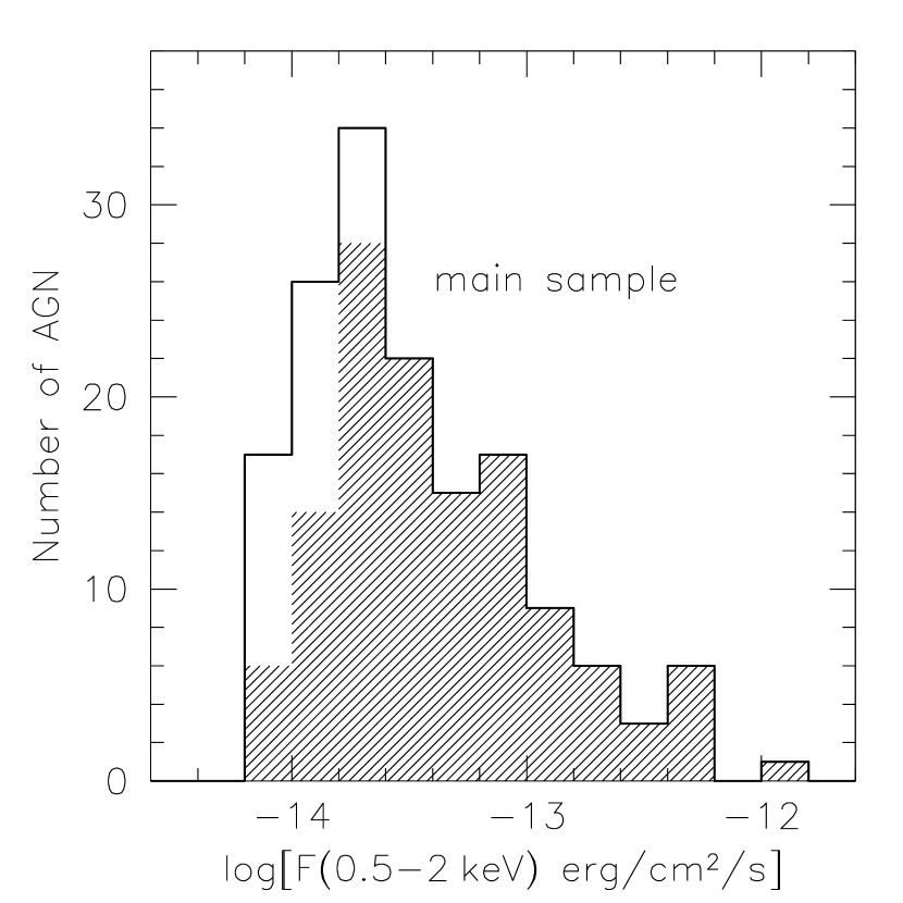
Figure 7.— Distribution of X-ray fluxes (hatched histogram) and upper limits (open histogram) for the SDSS main sample.

Table 1 gives the X-ray observation ID (column 3), effective exposure time (4), off-axis angle (5), total source counts (6), logarithm of the 0.5–2.0 keV flux (8), logarithm of the rest frame 2 keV monochromatic flux – $f_{\textrm{\scriptsize{2\,keV}}}$, not band-pass corrected (9), and logarithm of the rest frame 2.0 keV monochromatic luminosity – $l_{x}$, band-pass corrected (11) for each source in the main SDSS catalog. The 0.5–2 keV flux histogram of the main SDSS sample is shown in Figure 7. The soft X-ray detection limit for the inner 19^′ of the medium-deep ROSAT observations used here is $\sim$$2\times 10^{-14}$ erg cm^-2 s^-1. The fluxes were estimated using PIMMS assuming a power-law X-ray spectrum with photon index $\Gamma=2$ and the Galactic hydrogen column density obtained by Stark et al. (1992). Previous studies suggest that AGN photon indices do not vary systematically with redshift (e.g., Page et al., 2003; Vignali et al., 2003), although the scatter ($\sim$0.5) around the mean value is substantial for all redshifts. Assuming a constant $\Gamma$, when in reality $1.5<\Gamma<2.5$ for the different sources, affects our flux measurements by $\lesssim 4$%. Four of the selected 155 SDSS AGNs were the targets of their respective ROSAT pointed observations (marked by note 1 in Table 1). Their inclusion in the main sample could have a small effect on the sample correlations, as the four AGNs do not comply with our selection criteria – optically selected AGNs serendipitously observed in medium-deep ROSAT pointings. Three of the four AGNs are not substantially different in their rest-frame UV and X-ray properties from the rest of the sample, while SDSS J1701$+$6412 is the UV-brightest AGN in the main sample. We opt to retain the four ROSAT targets in the main sample, while ensuring that their presence has no material effect on any of our conclusions (see § 3.2 and § 3.3).

A total of 40 of the 155 SDSS AGNs (26%) were not detected in the 0.5–2.0 keV band by ROSAT. One of the 40 SDSS AGNs, SDSS J1400$+$6225, is not detected by ROSAT but is detected serendipitously on CCD S2 of a Chandra ACIS-S (Garmire et al., 2003) observation. We used ACIS Extract (Broos et al., 2004), which utilizes Chandra Interactive Analysis of Observations (CIAO v.3.0.2) tools, to estimate the 0.5–2.0 keV flux. Nine additional AGNs with ROSAT upper limits were serendipitously detected in XMM-Newton (Jansen et al., 2001) observations, as indicated in column (3) of Table 1. We use the count rates in the 0.5–2 keV band of the first XMM-Newton serendipitous source catalog – 1XMM SSC (Watson et al., 2003), whenever available (four sources), to obtain the XMM-Newton fluxes. For the remaining five XMM-Newton detected sources which are not in 1XMM SSC, we use the source lists provided by the standard XMM-Newton processing to extract the 0.5–2.0 keV count rates. When a source is detected by more than one XMM-Newton European Photon Imaging Camera (EPIC) instrument (Strüder et al., 2001), we average the estimated fluxes weighting by the quoted errors and report the MOS total counts and effective exposure times in Table 1. An additional 14 sources detected by ROSAT are also detected by XMM-Newton. The 0.5–2.0 keV fluxes of these 14 AGNs agree within 0.4 dex (a factor of  2.5) in 12 of the cases, and the XMM-Newton detections are more likely to be brighter by $\sim$30%. Taking into account that four of the ROSAT detections are 2–3$\sigma$ and that AGNs are variable on scales of hours to years (see the discussion of AGN X-ray variability in $\S$ 3.5.1), we consider this agreement adequate for inclusion of the XMM-Newton detected AGNs with no ROSAT detections into our sample.

A total of 14 AGNs in our main sample have XMM-Newton (13/14) or Chandra (1/14) detections replacing the ROSAT upper limits (10/14) or low-confidence/cluster-contaminated detections (4/14). The XMM-Newton/Chandra observations could be more likely to “catch” the SDSS AGNs in a high-luminosity state, if the difference between the ROSAT limiting flux and the XMM-Newton/Chandra detection flux is sufficiently small in comparison to AGN variability. Four of the 14 AGNs with XMM-Newton/Chandra detections have fluxes above their ROSAT limits ($\sim$30% higher) and could have been detected with XMM-Newton/Chandra only because they were in a high-luminosity state. The remaining ten AGNs were detected in more-sensitive XMM-Newton/Chandra observations. On account of these possible “high-state” detections and the tendency of some XMM-Newton detections to provide brighter 0.5–2.0 keV fluxes than the corresponding ROSAT detections, we will consider the effect of excluding all 14 XMM-Newton/Chandra detected AGNs on the subsequent correlations.

2.3. The High-Redshift Sample

To increase the redshift and luminosity coverage of the optically selected AGN sample, we add an auxiliary sample of 36 AGNs at $z>4$. These high-$z$ AGNs were selected from 44 AGNs specifically targeted for X-ray imaging with Chandra (19 SDSS AGNs, 16 Palomar Digital Sky Survey AGNs; Djorgovski et al. 1998; and seven AGNs from the Automatic Plate Measuring facility survey, Irwin, McMahon, & Hazard, 1991) and XMM-Newton (2 SDSS AGNs) reported in Tables 3 and A1 of Vignali et al. (2003). The 36 high-$z$ AGNs were selected from the original 44 AGNs by excluding three strongly radio-loud ($R>1.6$) AGNs and five BAL AGNs. This sample is somewhat more heterogeneous in its optical selection (although all $z<5.4$ high-$z$ AGNs would have made the SDSS AGN target selection), contains only the highest rest-frame UV luminosity AGNs, and was specifically targeted for X-ray observations. Consequently we carefully consider the effect of its addition to the main sample on the rest-frame UV-X-ray relations reported below.

2.4. The Seyfert 1 Sample

As noted in § 1, the significance of UV-X-ray correlations depends on the range of luminosities probed for each redshift. The SDSS selects photometric targets for spectroscopic follow-up in two magnitude ranges – low-redshift targets are magnitude limited at $\emph{i}<19.1$ and high-redshift targets at $\emph{i}<20.2$. Mainly due to the large solid angle covered by the SDSS, but also on account of its two different optical flux limits, the main SDSS sample probes a luminosity range of at least an order of magnitude at each redshift, except at $z\lesssim 0.2$ and $z\gtrsim 3$. In order to increase the luminosity range for low-redshift AGNs, we consider an additional sample of Seyfert 1 galaxies with measurements from both IUE and ROSAT. The majority of objects were selected from the Seyfert 1 list of Walter & Fink (1993) to have direct monochromatic flux measurements at both 2675 Å and 2 keV (see their Table 1) and $L_{\textrm{\scriptsize{$\nu$}}}(\textrm{2500\,\AA})>10^{27.5}$ erg s^-1 Hz^-1. NGC 3516 (Kolman et al., 1993) was added to the Walter & Fink (1993) Seyfert 1 list, and the I Zw 1 measurements were replaced with recent, more accurate estimates from Gallo et al. (2004). The monochromatic flux measurements at 2675 Å were not corrected for host-galaxy contamination, which we expect to be small at this wavelength for most sources. We inspected visually a few high S/N IUE spectra which showed no strong host-galaxy features. To exclude strongly radio-loud objects we consider only Seyfert 1s with $L_{\textrm{\scriptsize{$\nu$}}}(\textrm{5\,GHz})<10^{25}$ W Hz^-1, where we use the 5 GHz fluxes from Walter & Fink (1993) and additional 1.4 GHz flux measurements (extrapolated to 5 GHz) from NED, and exclude all Seyferts with unknown radio flux from FIRST or NVSS. Our final Seyfert 1 list consists of 37 AGNs. This sample is not biased in the sense that it includes only X-ray detections of known optical AGNs. It is not, however, purely optically selected; consequently, we evaluate all correlations with and without the Sy 1 subsample, to control for any possible systematics.

3. Correlation Analysis

3.1. Detection Fractions

A high X-ray detection fraction, which minimizes the effects of systematic pattern censoring and statistical assumptions, is essential for accurate determination of AGN UV-X-ray properties (see § 1). As can be seen in Figure 7, most sources with $F$${}_{\textrm{\scriptsize{(0.5-2\,keV)}}}$$>2\times 10^{-14}$ erg cm^-2 s^-1 are detected for an overall detection fraction of 126/155 (81%) in the main SDSS sample. The X-ray detection fractions (X-ray detected vs. total number) for the main, high-$z$ and combined (main, high-$z$, and Sy 1) samples are given in Table 2.

Figure 8.— The 2 keV vs. 2500 Å monochromatic luminosities for the SDSS main sample (solid circles), the high-$z$ sample (open squares), and the Sy 1 sample (open triangles). Arrows indicate upper limits. The solid line is the best-fit linear relation for the combined sample: $l_{\textrm{\scriptsize{x}}}=0.648l_{\textrm{\scriptsize{uv}}}+6.734$, and the dotted line is an arbitrarily normalized line with a slope of one.

3.2. Monochromatic Optical/UV and X-ray Luminosities

Figure 8 shows the relation between the 2 keV and 2500 Å monochromatic luminosities. The correlation is significant at the 11.5$\sigma$ (7.4$\sigma$) level, after the redshift dependence of both quantities and all upper limits are taken into account for the combined sample of 228 AGNs (the main SDSS sample of 155 AGNs). The partial Kendall’s correlation coefficient (Akritas & Siebert, 1996) is $\tau$${}_{\textrm{\scriptsize{12,3}}}$=0.38 ($\tau$${}_{\textrm{\scriptsize{12,3}}}$=0.28) for the combined (main) sample (see Table 3).

In order to test the partial-correlation method, we created mock datasets with variable dispersion and strong redshift dependence. We consider cases of (1) no relation between the dependent and independent variables and (2) a linear relation between the dependent and independent variables. In both cases we assume that the UV monochromatic luminosity is a polynomial function of redshift with a luminosity range of about an order of magnitude at each redshift, which includes a normally distributed dispersion (with standard deviation equal to the observed regression residuals from Table 3) to both the UV and X-ray monochromatic luminosities to simulate the uncertainty due to variability and measurement errors. The “true relation” simulation further assumes that Eqns. 1–3 given below hold, while the “no relation” simulation assumes that the X-ray monochromatic luminosity is a different polynomial function of redshift. When we match the observed redshift distribution and number of X-ray upper limits, we confirm the existence of the mock-linear relations with similar statistical significance to the significance found for the real datasets, $\sim$12–14$\sigma$ in the mock-combined and $\sim$8–10$\sigma$ in the mock-main simulated samples, weakly dependent on the ratio (varying between 0.5 and 2.0 in our simulations) of dispersions assumed for the dependent and independent variables.

For “no relation” simulations, spurious correlations of up to 4$\sigma$ in the mock-main and up to 7$\sigma$ in the mock-combined sample are possible. The apparent high significance of the “no-relation” simulations is caused by our lack of knowledge of the true mean dependence of the monochromatic luminosity on redshift in the UV and X-ray bands separately, combined with the observational constraint on the range of luminosities probed at each redshift. The simulation set-up is further affected by the fact the observations constrain only the total dispersions along the $l_{\textrm{\scriptsize{x}}}$–$l_{\textrm{\scriptsize{uv}}}$, $l_{\textrm{\scriptsize{uv}}}$–$z$, and $l_{\textrm{\scriptsize{x}}}$–$z$ relations, without strong constraints on the contribution of variability and measurement error. By necessity, the polynomial fits we use in the simulation to represent the mean $l_{\textrm{\scriptsize{uv}}}$–$z$ and $l_{\textrm{\scriptsize{x}}}$–$z$ relations are very similar, and consequently simulations with significant spurious correlations are possible. However, in no simulation where we match the observed $l_{\textrm{\scriptsize{uv}}}$–$z$ and $l_{\textrm{\scriptsize{x}}}$–$z$ distributions (in both their mean relations and dispersions) as well as the observed $l_{\textrm{\scriptsize{x}}}$–$l_{\textrm{\scriptsize{uv}}}$ dispersion, are the “no relation” correlations found significant enough to cause the observed $l_{\textrm{\scriptsize{x}}}$–$l_{\textrm{\scriptsize{uv}}}$ correlations. Additionally, in all simulated cases the significance of the “true relation” simulation is sufficiently higher than the corresponding “no relation” case, allowing for easy distinction between the two. Consequently, we are convinced that 11.5$\sigma$ (7.4$\sigma$) level correlations found for the combined (main) samples are unlikely to arise on account of the strong redshift dependence of the UV and X-ray monochromatic luminosities.

The best-fit relations, assuming no redshift dependence (see the discussion below), are

$$l_{\textrm{\scriptsize{x}}}(l_{\textrm{\scriptsize{uv}}})=(0.645\pm 0.034)l_{\textrm{\scriptsize{uv}}}+(6.851\pm 1.036)$$

main sample (1)

$$l_{\textrm{\scriptsize{x}}}(l_{\textrm{\scriptsize{uv}}})=(0.639\pm 0.026)l_{\textrm{\scriptsize{uv}}}+(7.026\pm 0.804)$$

main$$+ z$$high- (2)

$$l_{\textrm{\scriptsize{x}}}(l_{\textrm{\scriptsize{uv}}})=(0.648\pm 0.021)l_{\textrm{\scriptsize{uv}}}+(6.734\pm 0.643)$$

main$$+ z +$$high-Sy 1 (3)

(the excess precision quoted is useful for plotting purposes). In all cases the fits given above were obtained using the EM algorithm for censored data from ASURV; the Buckley-James method from ASURV returns results consistent within $1\sigma$. The resulting slope is less than one in all cases, implying a changing ratio between the 2 keV and 2500 Å monochromatic luminosities with rest-frame UV luminosity. The residual scatters around the linear relationships are 0.39, 0.37, and 0.36 (in $\log$ units) for the main, main$+$high-$z$, and combined samples, respectively (see Table 3). Removing the four AGNs which were targets of ROSAT pointings or the 14 AGNs with XMM-Newton/Chandra X-ray photometry, has no material effect on the parameters of the linear regression and only slightly decreases the significance of the correlation (on account of the decrease in sample size and the consequent slight increase in the fraction of upper limits when $\gtrsim 10$ detections are excluded). In order to check for any effect of the unidentified HiBALs/LoBALs remaining in our sample, we exclude the 9 steepest $\alpha_{\textrm{\scriptsize{ox}}}$ sources with $z<1.55$ from the main sample before performing the correlation. The linear regression parameters for the main sample remain unchanged within the quoted errors, with $l_{\textrm{\scriptsize{x}}}=(0.65\pm 0.03)l_{\textrm{\scriptsize{uv}}}+(6.8\pm 1.0)$. Similarly for the combined sample, assuming a 10% observed HiBAL fraction and taking into account that there are 146 AGNs without C IV coverage, we exclude the 15 steepest $\alpha_{\textrm{\scriptsize{ox}}}$ sources with $z<1.55$ or $z>4.8$, before repeating the correlation analysis. We find $l_{\textrm{\scriptsize{x}}}=(0.63\pm 0.02)l_{\textrm{\scriptsize{uv}}}+(7.3\pm 0.6)$, consistent within 1$\sigma$ with Eqn. 3 above. Removing an additional 10 SDSS AGNs from the main sample with some UV absorption which do not satisfy the BAL criteria (see § 2.1) also has no effect on the correlation parameters, yielding $l_{\textrm{\scriptsize{x}}}=(0.65\pm 0.04)l_{\textrm{\scriptsize{uv}}}+(6.7\pm 1.1)$. Constraining the linear regression to the 81 AGNs with $1.55<z<4.80$, where BAL AGNs are easy to exclude using the absorption blueward of C IV, we obtain a slightly shallower slope for the $l_{\textrm{\scriptsize{x}}}$–$l_{\textrm{\scriptsize{uv}}}$ correlation, $l_{\textrm{\scriptsize{x}}}=(0.58\pm 0.06)l_{\textrm{\scriptsize{uv}}}+(8.8\pm 1.8)$, consistent with Eqns. 1–3 within $1\sigma$.

Figure 9.— Positions of the main-sample AGNs in the relative g$-$i color, $\Delta(g-i)$ vs. redshift diagram. The dashed line represents SMC-type reddening as a function of redshift with $E(B-V)=0.04$ shifted redward by 0.2 to satisfy the Richards et al. (2003a) dust-reddening definition. AGNs to the right of the dashed line can be considered to be dust reddened (see Figure 6 of Richards et al., 2003a). Note that the Lyman limit affects the g magnitudes of the four AGNs with $z>3.1$, rendering their relative colors unreliable.

In order to probe the effects of any dust absorption in the rest-frame UV on the $l_{\textrm{\scriptsize{x}}}$–$l_{\textrm{\scriptsize{uv}}}$ relation, we use the relative g$-$i AGN color, $\Delta(g-i)$. Richards et al. (2003a) have shown that a $\Delta(g-i)$ vs. $z$ diagram, like the one presented in Figure 9, can be used to define a dust reddened AGN subsample (to the right of the dashed line, see their Figure 6). Excluding the 17 AGNs considered dust-reddened according to Richards et al. (2003a) definition has no effect on the parameters of the $l_{\textrm{\scriptsize{x}}}$–$l_{\textrm{\scriptsize{uv}}}$ correlation in the main sample, $l_{\textrm{\scriptsize{x}}}=(0.65\pm 0.04)l_{\textrm{\scriptsize{uv}}}+(6.8\pm 1.1)$.

3.3. $\alpha$${}_{\textrm{\scriptsize{ox}}}$ – primary dependence on luminosity rather than redshift

Distributions of $\alpha$${}_{\textrm{\scriptsize{ox}}}$ are presented in Figure 10 for the main SDSS (top) and the high-$z$ and Sy 1 (bottom) samples. The main SDSS sample has a median $\alpha_{\textrm{\scriptsize{ox}}}=-1.51$, compared to $\alpha_{\textrm{\scriptsize{ox}}}=-1.72$ for the high-$z$ sample and $\alpha_{\textrm{\scriptsize{ox}}}=-1.34$ for the Sy 1 sample. In addition, as can be seen from the numbers on the top of each bin in the top histogram of Figure 10, lower monochromatic luminosity AGNs ($l_{\textrm{\scriptsize{uv}}}<30.5$, left number) have flatter $\alpha_{\textrm{\scriptsize{ox}}}$ indices compared to higher monochromatic luminosity AGNs ($l_{\textrm{\scriptsize{uv}}}>30.5$, right number). It is therefore apparent that $\alpha_{\textrm{\scriptsize{ox}}}$ is correlated with rest-frame monochromatic UV luminosity and/or redshift. We will show below that the primary dependence of $\alpha$${}_{\textrm{\scriptsize{ox}}}$ is on rest-frame monochromatic UV luminosity, while the redshift dependence is insignificant.

Figures 11 and 12 present the $\alpha$${}_{\textrm{\scriptsize{ox}}}$ dependence on $l$${}_{\textrm{\scriptsize{uv}}}$ and redshift. The optical/UV-to-X-ray index $\alpha$${}_{\textrm{\scriptsize{ox}}}$ depends primarily on $l$${}_{\textrm{\scriptsize{uv}}}$ with a linear partial correlation coefficient of $\tau_{\textrm{\scriptsize{12,3}}}=-0.33$ ($\tau_{\textrm{\scriptsize{12,3}}}=-0.30$) at a significance level of 10.6$\sigma$ (7.4$\sigma$) for the combined (main) sample. Table 3 presents the partial correlation statistics for various AGN subsamples. Taking into account that the $\alpha$${}_{\textrm{\scriptsize{ox}}}$–$z$ correlation coefficient changes from negative (main and main$+$high-$z$ samples) to positive (combined sample), and that the correlation significance level is always $<1.1\sigma$, our Monte Carlo simulations suggest that any apparent correlation could arise by chance due to the third variable ($l$${}_{\textrm{\scriptsize{uv}}}$) dependence. To illustrate this using the combined sample, we show in Figure 13 the residuals for an assumed $\alpha$${}_{\textrm{\scriptsize{ox}}}$ dependence on a single parameter – $l_{\textrm{\scriptsize{uv}}}$ in the top panel and $z$ in the bottom. The structure of the residuals confirms that an $\alpha$${}_{\textrm{\scriptsize{ox}}}$ dependence on $l_{\textrm{\scriptsize{uv}}}$ only is adequate to describe the observed variation in $\alpha$${}_{\textrm{\scriptsize{ox}}}$, while a redshift dependence alone is inadequate (as shown by the systematic residuals). In fact, if we attempt to fit a relation of the form, $\alpha_{\textrm{\scriptsize{ox}}}=Al_{\textrm{\scriptsize{uv}}}+Bz+C$ to the combined sample, the result is a fit with $B$ equal to zero within the errors. The linear regression fits, taking into account the $\alpha$${}_{\textrm{\scriptsize{ox}}}$ upper limits and ignoring any redshift dependence, are

$$\alpha_{\textrm{\scriptsize{ox}}}(l_{\textrm{\scriptsize{uv}}})=-(0.136\pm 0.013)l_{\textrm{\scriptsize{uv}}}+(2.630\pm 0.398)$$

main sample (4)

$$\alpha_{\textrm{\scriptsize{ox}}}(l_{\textrm{\scriptsize{uv}}})=-(0.139\pm 0.010)l_{\textrm{\scriptsize{uv}}}+(2.703\pm 0.309)$$

main$$+ z$$high- (5)

$$\alpha_{\textrm{\scriptsize{ox}}}(l_{\textrm{\scriptsize{uv}}})=-(0.136\pm 0.008)l_{\textrm{\scriptsize{uv}}}+(2.616\pm 0.249)$$

main$$+ z +$$high-Sy 1 (6)

(the excess precision quoted is useful for plotting purposes). The residual scatter around the linear relations is 0.14 in $\log$ units for all samples. The $\alpha$${}_{\textrm{\scriptsize{ox}}}$–$l$${}_{\textrm{\scriptsize{uv}}}$ slopes for all samples are consistent with those inferred from the $l$${}_{\textrm{\scriptsize{x}}}$–$l$${}_{\textrm{\scriptsize{uv}}}$ regressions in § 3.2.

Figure 10.— $\alpha$${}_{\textrm{\scriptsize{ox}}}$ distributions for the main SDSS (top), high-$z$ (bottom, solid line), and Sy 1 (bottom, dashed line) samples. The hatched histograms indicate X-ray upper limits. The two numbers on the top of each bin in the top histogram give the numbers of AGNs with $l_{\textrm{\scriptsize{uv}}}<30.5$ (left) and $l_{\textrm{\scriptsize{uv}}}>30.5$ (right) in that bin.

Comparison with previous work is not entirely straightforward, since the sample selections, X-ray detection fractions, pattern censoring, and control of other systematics in previous studies differ substantially from those presented here. Wilkes et al. (1994) obtain $\alpha$${}_{\textrm{\scriptsize{ox}}}$–$l$${}_{\textrm{\scriptsize{uv}}}$ slopes ranging from $-0.1$ to $-0.2$ for various AGN subsamples, selected from a heterogeneous and incomplete sample of 343 AGNs, the majority of which were optically selected and observed with Einstein. For a subsample of 272 RQ, $l_{\textrm{\scriptsize{uv}}}>29.0$ AGNs, Wilkes et al. (1994) find $\alpha_{\textrm{\scriptsize{ox}}}\propto-(0.15\pm 0.03)l_{\textrm{\scriptsize{uv}}}$ (see their Figure 14a), which is consistent with Eqns.(4)–(6) above. Green et al. (1995) use a stacking technique to obtain an $\alpha$${}_{\textrm{\scriptsize{ox}}}$–$l$${}_{\textrm{\scriptsize{uv}}}$ relation for 908 Large Bright Quasar Survey AGNs with RASS coverage, only 10% of which have X-ray detections. Binning in luminosity and redshift, and assuming no redshift dependence, they obtain $\alpha_{\textrm{\scriptsize{ox}}}\propto-(0.08\pm 0.02)l_{\textrm{\scriptsize{uv}}}$, which is consistent with our results within 3$\sigma$, but the comparison is inappropriate since their sample includes both RL and BAL AGNs. The corresponding slope for the $\alpha$${}_{\textrm{\scriptsize{ox}}}$–$l$${}_{\textrm{\scriptsize{uv}}}$ relation found by VBS03 and updated by Vignali et al. (2003) is $-0.095\pm 0.021$ for the SDSS EDR sample, significant at the 3–4$\sigma$ level. The higher significance of the $\alpha$${}_{\textrm{\scriptsize{ox}}}$–$l$${}_{\textrm{\scriptsize{uv}}}$ anti-correlation found in our new sample is a result of the increased monochromatic luminosity and redshift coverage, as well as the increased X-ray detection fraction; the 2$\sigma$ difference in the $\alpha$${}_{\textrm{\scriptsize{ox}}}$–$l$${}_{\textrm{\scriptsize{uv}}}$ slope is probably caused by the higher fraction of X-ray upper limits in the VBS03 sample ($\sim$50% in VBS03 and Vignali et al., 2003). Aside from the higher statistical significance of our current results, we also consider them to be less prone to systematic errors of the type described in § 1.

Figure 11.— Top: $\alpha$${}_{\textrm{\scriptsize{ox}}}$ dependence on the 2500 Å monochromatic luminosity. The main sample is given with solid circles, the high-$z$ sample with open squares, and the Sy 1 sample with open triangles; arrows in the top panel indicate $2\,$keV upper limits. The solid line is the linear relation found for the combined sample (Eqn. 6), and the dotted line is the corresponding relation from Vignali et al. (2003, their Eqn. 4). The anti-correlation is significant at the 10.6$\sigma$ level for the combined sample. Bottom: Kaplan-Meier estimator of the mean $\alpha$${}_{\textrm{\scriptsize{ox}}}$ as a function of $l$${}_{\textrm{\scriptsize{uv}}}$. The numbers at the top indicate the centers of the $l$${}_{\textrm{\scriptsize{uv}}}$ bins and the number of limits vs. the total number of AGNs in each bin.

Based on the $\alpha_{\textrm{\scriptsize{ox}}}-\alpha_{\textrm{\scriptsize{ox}}}(l_{\textrm{\scriptsize{uv}}})$ residuals, we can estimate the maximum possible residual dependence of $\alpha_{\textrm{\scriptsize{ox}}}$ on redshift and the corresponding maximum possible variation of the ratio of UV-to-X-ray flux, $r=F_{\nu}(\textrm{2500\,\AA})/F_{\nu}(\textrm{2\,keV})$. Using the Kaplan-Meier estimator means of the $\alpha_{\textrm{\scriptsize{ox}}}-\alpha_{\textrm{\scriptsize{ox}}}(l_{\textrm{\scriptsize{uv}}})$ residuals in nine redshift bins (see inset plot in the top panel of Figure 13), we obtain the weighted linear regression $\left<\alpha_{\textrm{\scriptsize{ox}}}-\alpha_{\textrm{\scriptsize{ox}}}(l_{\textrm{\scriptsize{uv}}})\right>=$ $(0.005\pm 0.012)z+(-0.010\pm 0.023)$. The slope is consistent with zero, which again indicates that there is no need for an additional redshift dependence. According to the above linear regression, we expect $\alpha_{\textrm{\scriptsize{ox}}}$ to vary by no more than 0.03 between the redshifts of 0 and 5. By definition, $r=F_{\nu}(\textrm{2500\,\AA})/F_{\nu}(\textrm{2\,keV})=10^{2.606\alpha_{\textrm{\scriptsize{ox}}}}$, and differentiating this with respect to $\alpha$${}_{\textrm{\scriptsize{ox}}}$, we have $\delta r/r=2.606(\delta\alpha_{\textrm{\scriptsize{ox}}})\log_{e}(10)\approx 6(\delta\alpha_{\textrm{\scriptsize{ox}}})\approx 0.2$, for $\delta\alpha_{\textrm{\scriptsize{ox}}}=0.03$. This implies that the ratio of rest-frame UV-to-X-ray flux could only change by $\lesssim$20% with cosmic time from $z\approx 0-5$. Similar analysis applied to the $\alpha_{\textrm{\scriptsize{ox}}}-\alpha_{\textrm{\scriptsize{ox}}}(z)$ residuals (see inset plot in the right panel of Figure 13) confirms that redshift alone cannot be responsible for the observed variation in $\alpha_{\textrm{\scriptsize{ox}}}$. The $\alpha_{\textrm{\scriptsize{ox}}}-\alpha_{\textrm{\scriptsize{ox}}}(z)$ residuals show a systematic variation of $\sim$0.2 between monochromatic luminosities $l_{\textrm{\scriptsize{uv}}}=28.5$ and $l_{\textrm{\scriptsize{uv}}}=31.8$.

Figure 12.— Top: The correlation of $\alpha$${}_{\textrm{\scriptsize{ox}}}$ with $z$ is only $\sim$1$\sigma$ significant if the $l$${}_{\textrm{\scriptsize{uv}}}$ dependence is taken into account (see § 3.3). Bottom: Kaplan-Meier estimator of the mean $\alpha$${}_{\textrm{\scriptsize{ox}}}$ as a function of redshift. Symbols and numbers are as in Figure 11.

Figure 13.— Single-parameter fit residuals for an $\alpha$${}_{\textrm{\scriptsize{ox}}}$ dependence on $l_{\textrm{\scriptsize{uv}}}$ (top) or $z$ (bottom) for the combined sample. The systematic residuals in the right plot support the idea that redshift alone cannot be responsible for the observed variation in $\alpha$${}_{\textrm{\scriptsize{ox}}}$. Symbols are as in Figure 11. The small inset plots in each panel give the Kaplan-Meier estimators of the means of the $\alpha_{\textrm{\scriptsize{ox}}}-\alpha_{\textrm{\scriptsize{ox}}}(l_{\textrm{\scriptsize{uv}}})$ (top) and $\alpha_{\textrm{\scriptsize{ox}}}-\alpha_{\textrm{\scriptsize{ox}}}(z)$ (bottom) residuals in the same redshift and monochromatic luminosity bins as in Figures 12 and 11, respectively. The dashed lines in each inset plot correspond to the weighted linear regression fits, $\left<\alpha_{\textrm{\scriptsize{ox}}}-\alpha_{\textrm{\scriptsize{ox}}}(l_{\textrm{\scriptsize{uv}}})\right>=(0.005\pm 0.012)z+(-0.010\pm 0.023)$ (top) and $\left<\alpha_{\textrm{\scriptsize{ox}}}-\alpha_{\textrm{\scriptsize{ox}}}(z)\right>=(-0.039\pm 0.020)l_{uv}+(1.184\pm 0.603)$ (bottom).

Figure 14 shows the distributions of $\alpha_{\textrm{\scriptsize{ox}}}-\alpha_{\textrm{\scriptsize{ox}}}(l_{\textrm{\scriptsize{uv}}})$ residuals, adjusted for the luminosity dependence of $\alpha_{\textrm{\scriptsize{ox}}}$ (using Eqn. 6), for both the combined sample and a $1.55<z<4.8$ subsample (for which all HiBALs can be identified using SDSS spectroscopy). Both distributions have been rescaled to $N=228$, the total number of AGNs in the combined sample. The slight tendency of the combined-sample distribution towards more negative $\alpha_{\textrm{\scriptsize{ox}}}-\alpha_{\textrm{\scriptsize{ox}}}(l_{\textrm{\scriptsize{uv}}})$ values is probably a result of the $\sim$9–15 unidentified BALs which remain in the sample due to lack of C IV spectroscopic coverage for $z<1.55$ and $z>4.8$. Proper comparison (i.e., one that takes into account the upper limits) of the two distributions with Gehan and logrank tests from ASURV shows that they are indistinguishable, implying that our combined sample does not contain more than a few percent obscured or X-ray weak AGNs. The dotted curve in the top panel of Figure 14 is a Gaussian representation of the combined-sample residuals with a mean of 0.017 and a standard deviation of 0.11 (compared to 0.14 obtained from the linear regression of the combined sample). The Gaussian parameterization provides a reasonable representation of the residuals in both the observed (shown in Figure 14) and the binned differential Kaplan-Meier distributions. It is unlikely that we can determine whether a different parametric distribution (e.g., a Lorentzian) will provide a better fit, since the tails of the distribution are uncertain due to the small number of objects. There is no evidence of significant skewness of the $\alpha_{\textrm{\scriptsize{ox}}}$ distribution, after correction for the luminosity dependence of $\alpha_{\textrm{\scriptsize{ox}}}$. If a significant number of obscured AGNs remained in our sample, we would see an extended leftward tail of the $\alpha_{\textrm{\scriptsize{ox}}}-\alpha_{\textrm{\scriptsize{ox}}}(l_{\textrm{\scriptsize{uv}}})$ residuals (if the absorbed AGNs had X-ray detections, as in Figure 1 of Brandt, Laor, & Wills, 2000), or a significant skewness of the distribution if only upper limits were available for the BAL AGNs. We suspect that the skewness of the $\alpha_{\textrm{\scriptsize{ox}}}$ distribution seen by Avni & Tananbaum (1986, see their Figure 1, with the $x$-axis reversed) is a result of the presence of obscured (and possibly a larger fraction of RL) AGNs in their sample. The bottom panel of Figure 14 presents the $\alpha_{\textrm{\scriptsize{ox}}}-\left<\alpha_{\textrm{\scriptsize{ox}}}\right>$ residuals, where $\left<\alpha_{\textrm{\scriptsize{ox}}}\right>=-1.514$ is the Kaplan-Meier average of the combined sample, assuming no $l$${}_{\textrm{\scriptsize{uv}}}$ and no redshift dependence. The broad distribution is a result of ignoring the $\alpha$${}_{\textrm{\scriptsize{ox}}}$–$l$${}_{\textrm{\scriptsize{uv}}}$ anti-correlation in a sample with a large range of luminosities.

Figure 14.— Distributions of the $\alpha_{\textrm{\scriptsize{ox}}}$ residuals after adjusting for the $l_{\textrm{\scriptsize{uv}}}$ dependence (top) or the average $\alpha_{\textrm{\scriptsize{ox}}}$ (bottom, assuming no $l_{\textrm{\scriptsize{uv}}}$ or $z$ dependence). The hatched histogram in the top panel represents the 228 AGNs from the combined sample; the open histogram represents the 81 AGNs with $1.55<z<4.8$ (normalized to $N=228$ for comparison), for which all BAL AGNs can be identified using the SDSS spectroscopy. The dotted Gaussian shown in both panels is centered at $\alpha_{\textrm{\scriptsize{ox}}}-\alpha_{\textrm{\scriptsize{ox}}}(l_{\textrm{\scriptsize{uv}}})=0.017$ and has a standard deviation of 0.11. The two numbers on the tops of some histogram bins show the number of AGNs in each bin with X-ray limits in the combined sample (left number) and the $1.55<z<4.8$ subsample (right number, no normalization was applied).

Eqns. 4–6 show that, within the quoted uncertainties, the same slope and intercept for the $\alpha$${}_{\textrm{\scriptsize{ox}}}$–$l$${}_{\textrm{\scriptsize{uv}}}$ relation are present for the main, main$+$high-$z$, and combined samples. As detailed in § 3.2, these parameter estimates are also unaffected by the exclusion of the 14 XMM-Newton/Chandra detected AGNs, the four ROSAT targets, the 9–15 steepest $\alpha$${}_{\textrm{\scriptsize{ox}}}$ AGNs (at the appropriate redshifts) to check for any effect of the unidentified HiBALs, an additional 10 AGNs with some UV absorption, or the 17 AGNs considered dust-reddened by the Richards et al. (2003a) criterion. The strength of the correlations is slightly lower (7.2–9.4$\sigma$ level for the different samples) if the 14 XMM-Newton/Chandra AGNs are excluded, since this decreases the sample size by $\sim$7% and the detection fraction by $\sim$1–2%. If we do not correct for the host-galaxy contamination in low-luminosity AGNs from the main SDSS sample, Eqn. 4 above would have a somewhat shallower slope of $-0.128\pm 0.014$ and an intercept of $2.377\pm 0.417$. The effect is in the expected direction (taking into account the artificial increase in $l$${}_{\textrm{\scriptsize{uv}}}$ and steepening of $\alpha$${}_{\textrm{\scriptsize{ox}}}$ for the affected AGNs), and its size ($\lesssim 1\sigma$) is determined by the fact that only $\sim$17% of the 155 SDSS AGNs have host-galaxy correction $>$5%. Even if all Sy 1 AGNs need similar host galaxy corrections, their effect on the $\alpha$${}_{\textrm{\scriptsize{ox}}}$–$l$${}_{\textrm{\scriptsize{uv}}}$ anti-correlation parameters will be equally small, as they represent only 16% of the full sample (37/228).

Figure 15.— Single-parameter fit residuals for an $\alpha$${}_{\textrm{\scriptsize{ox}}}$ dependence on $l_{\textrm{\scriptsize{uv}}}$ (from Eqn. 6) vs. $\Delta(g-i)$ for the main SDSS sample (solid circles). The four $z>3.1$ main-sample AGNs with $\Delta(g-i)$ values affected by the Lyman limit are excluded. Arrows indicate X-ray upper limits. The Kaplan-Meier estimators of the mean $\alpha_{\textrm{\scriptsize{ox}}}-\alpha_{\textrm{\scriptsize{ox}}}(l_{\textrm{\scriptsize{uv}}})$ in four $\Delta(g-i)$ bins, given with large filled squares, show that $\alpha_{\textrm{\scriptsize{ox}}}-\alpha_{\textrm{\scriptsize{ox}}}(l_{\textrm{\scriptsize{uv}}})$ is not strongly correlated with $\Delta(g-i)$ over the range where we have coverage.

Figure 15 presents the $\alpha_{\textrm{\scriptsize{ox}}}-\alpha_{\textrm{\scriptsize{ox}}}(l_{\textrm{\scriptsize{uv}}})$ residuals of the main SDSS sample vs. the redshift-corrected g$-$i color, $\Delta(g-i)$. Although the redder SDSS AGNs with $\Delta(g-i)>0$ appear to be more likely to have $\alpha_{\textrm{\scriptsize{ox}}}$ limits rather than detections (partially because they have fainter i magnitudes; see Figure 2), no trend of the Kaplan-Meier estimators of the mean $\alpha_{\textrm{\scriptsize{ox}}}-\alpha_{\textrm{\scriptsize{ox}}}(l_{\textrm{\scriptsize{uv}}})$ residuals is apparent when we bin the data in four $\Delta(g-i)$ bins (selected to have equal numbers of objects). A Spearman test on the individual data points returns a correlation coefficient of $-$0.14 with an 8% probability of the null hypothesis (no correlation) being correct. We conclude that any dust-reddening dependence of $\alpha_{\textrm{\scriptsize{ox}}}$ (in addition to the $l_{\textrm{\scriptsize{uv}}}$ dependence) must be weak for the main SDSS sample, at least over the $\Delta(g-i)$ range where we have significant source statistics.

3.4. Is the $\alpha$${}_{\textrm{\scriptsize{ox}}}$–$l$${}_{\textrm{\scriptsize{uv}}}$ Relation Non-linear?

Some studies of optical/UV and X-ray emission from AGNs suggest a possible non-linear dependence of $\alpha$${}_{\textrm{\scriptsize{ox}}}$ on $l$${}_{\textrm{\scriptsize{uv}}}$ (Wilkes et al., 1994; Anderson et al., 2003). Wilkes et al. (1994) observe that the $\alpha$${}_{\textrm{\scriptsize{ox}}}$–$l$${}_{\textrm{\scriptsize{uv}}}$ correlation found for the Einstein quasar database, $\alpha_{\textrm{\scriptsize{ox}}}\propto-0.11l_{\textrm{\scriptsize{uv}}}$, has a flatter slope, $\alpha_{\textrm{\scriptsize{ox}}}\propto-0.08l_{\textrm{\scriptsize{uv}}}$, if the sample is restricted to low-luminosity objects with $l_{\textrm{\scriptsize{uv}}}<29.5$. While the authors cannot rule out a non-linear relation, they suggest that the difference in slopes is likely caused by the varying host-galaxy contribution to the $l$${}_{\textrm{\scriptsize{uv}}}$ measurement at low redshift (which is accompanied, as expected, by a larger scatter in $\alpha$${}_{\textrm{\scriptsize{ox}}}$). Anderson et al. (2003) also report an observed tendency toward a non-linear $\alpha$${}_{\textrm{\scriptsize{ox}}}$–$l$${}_{\textrm{\scriptsize{uv}}}$ relation (note that they also use the term “non-linear” to refer to the fact that the slope of the linear $l$${}_{\textrm{\scriptsize{x}}}$–$l$${}_{\textrm{\scriptsize{uv}}}$ relation is less than one). The Anderson et al. (2003) sample contains $\sim$1158 bright ROSAT All Sky Survey (RASS) selected AGNs with broad-line SDSS counterparts. This sample is not optically selected; in fact it provides X-ray fluxes for only $\sim$10% of all SDSS AGNs, the majority of which are at low redshifts ($z<1$). The goal of the Anderson et al. (2003) paper was to present the first installment of a RASS-SDSS catalog; consequently the presented analysis of the $\alpha$${}_{\textrm{\scriptsize{ox}}}$–$l$${}_{\textrm{\scriptsize{uv}}}$ relation, as stated by the authors, was not intended to be conclusive. The effects not taken into account include sample selection biases, the statistical method which did not consider third-variable dependencies or the effect of unidentified BALs, and the effects of the varying dispersions in the optical/UV and X-ray bands (see § 3.5). To our knowledge, there is presently no conclusive evidence for a non-linear $\alpha$${}_{\textrm{\scriptsize{ox}}}$–$l$${}_{\textrm{\scriptsize{uv}}}$ correlation.

From Figure 11, it appears that the $\alpha$${}_{\textrm{\scriptsize{ox}}}$–$l$${}_{\textrm{\scriptsize{uv}}}$ correlation may be non-linear, with a flatter slope for $l_{\textrm{\scriptsize{uv}}}\lesssim 30.5$ and a steeper one at higher monochromatic luminosities. We checked this by performing linear regressions separately for two subsamples, separated at $l_{\textrm{\scriptsize{uv}}}=30.5$. The results shown below are based on the main$+$high-$z$ samples, excluding the Sy 1 sample which is not optically selected; the combined sample gives qualitatively the same results. We obtain a slope of $-0.09\pm 0.02$ for the $l_{\textrm{\scriptsize{uv}}}<30.5$ subsample, and $-0.13\pm 0.02$ for the $l_{\textrm{\scriptsize{uv}}}>30.5$ subsample. It appears that the slopes are different at the $\sim$2$\sigma$ level. From Figure 11, the main SDSS sample has five outlier points at low monochromatic luminosities (with $l_{\textrm{\scriptsize{uv}}}<29$ and $\alpha_{\textrm{\scriptsize{ox}}}<-1.46$), which could have influenced the anti-correlation found for $l_{\textrm{\scriptsize{uv}}}<30.5$ AGNs. If we exclude those points and repeat the analysis, we obtain slopes of $-0.12\pm 0.02$ and $-0.13\pm 0.02$ for the $l_{\textrm{\scriptsize{uv}}}<30.5$ and $l_{\textrm{\scriptsize{uv}}}>30.5$ subsamples, respectively, implying that the difference in slopes is likely an artifact of the addition of the five outlier AGNs rather than demonstrating a real difference. The five outliers are all nearby AGNs, with $z<0.22$, and most of them are probably X-ray absorbed Seyferts. Exclusion of the five outlier AGNs has a $1\sigma$ effect on the regression parameters in the combined sample, steepening the slope from $\alpha_{\textrm{\scriptsize{ox}}}\propto(-0.14\pm 0.01)l_{\textrm{\scriptsize{uv}}}$ to $\alpha_{\textrm{\scriptsize{ox}}}\propto(-0.15\pm 0.01)l_{\textrm{\scriptsize{uv}}}$. We conclude that the present sample does not offer significant evidence for a non-linear $\alpha$${}_{\textrm{\scriptsize{ox}}}$–$l$${}_{\textrm{\scriptsize{uv}}}$ relation.

3.5. Validating the Slope of the $l_{\textrm{\scriptsize{x}}}$–$l_{\textrm{\scriptsize{uv}}}$ Relation

Chanan (1983, C83), La Franca et al. (1995, F95), and Yuan, Siebert, & Brinkmann (1998, YSB98) explore the possibility that the intrinsic $l_{\textrm{\scriptsize{x}}}$–$l_{\textrm{\scriptsize{uv}}}$ relation has a slope of one. They propose that a larger dispersion in the rest-frame UV (relative to the X-ray) measurements, combined with the steep bright-end UV luminosity function, conspire to produce an $l_{\textrm{\scriptsize{x}}}$–$l_{\textrm{\scriptsize{uv}}}$ relation with a slope smaller than one and an apparent $\alpha$${}_{\textrm{\scriptsize{ox}}}$–$l_{\textrm{\scriptsize{uv}}}$ correlation. Both F95 and YSB98 assume Gaussian distributions of uncertainties independent of luminosity or redshift for $l_{\textrm{\scriptsize{x}}}$ and $l_{\textrm{\scriptsize{uv}}}$. They take the observed dispersion around a linear $l_{\textrm{\scriptsize{x}}}$–$l_{\textrm{\scriptsize{uv}}}$ relation to be $\sim$0.4–0.5 in $\log$ units, corresponding to a dispersion of 0.15–0.2 in the $\alpha$${}_{\textrm{\scriptsize{ox}}}$–$l_{\textrm{\scriptsize{uv}}}$ relation. This is presumably caused by dispersion in the optical/UV and X-ray measurements due to measurement error, variability, and intrinsic dispersion (related to differences in accretion modes and the conditions in the immediate AGN environment as well as the galaxy host). In order to fit their Einstein data with a linear $l_{\textrm{\scriptsize{x}}}$–$l_{\textrm{\scriptsize{uv}}}$ relation, F95 require a dispersion in the rest-frame monochromatic UV luminosity of $\sigma_{\textrm{\scriptsize{uv}}}\approx 0.34$ in $\log$ units (corresponding to 0.85 mag); the known causes of uncertainty in their sample (i.e., optical/UV photometric measurement error, assumed constant optical/UV spectral slope, and AGN variability) account for only 0.5 mag. Thus, the F95 conclusions depend on the assumption that the extra scatter observed around the linear $l_{\textrm{\scriptsize{x}}}$–$l_{\textrm{\scriptsize{uv}}}$ relation is due to extra dispersion in the optical/UV.

YSB98 and Yuan (1999) also assume that the observed dispersion in the $l_{\textrm{\scriptsize{x}}}$–$l_{\textrm{\scriptsize{uv}}}$ relation is largely due to Gaussian uncertainty in the optical/UV. In the notation of Yuan (1999), given intrinsic monochromatic luminosities of $\bar{l}_{\textrm{\scriptsize{x}}}$ and $\bar{l}_{\textrm{\scriptsize{uv}}}$ modified by (measurement-error, variability, and intrinsic) scatters of $\delta l_{\textrm{\scriptsize{x}}}$ and $\delta l_{\textrm{\scriptsize{uv}}}$, the observed monochromatic luminosities are $l_{\textrm{\scriptsize{x}}}=\bar{l}_{\textrm{\scriptsize{x}}}+\delta l_{\textrm{\scriptsize{x}}}$ and $l_{\textrm{\scriptsize{uv}}}=\bar{l}_{\textrm{\scriptsize{uv}}}+\delta l_{\textrm{\scriptsize{uv}}}$. The scatters $\delta l_{\textrm{\scriptsize{x}}}$ and $\delta l_{\textrm{\scriptsize{uv}}}$ are assumed to be independent of luminosity and redshift and well represented by Gaussian distributions with zero means and standard deviations of $\sigma_{\textrm{\scriptsize{x}}}$ and $\sigma_{\textrm{\scriptsize{uv}}}$. YSB98 and Yuan (1999) caution that a spurious $\alpha$${}_{\textrm{\scriptsize{ox}}}$–$l_{\textrm{\scriptsize{uv}}}$ relation could arise for samples with large optical/UV dispersions (with optical/UV-to-X-ray dispersion ratio, $R_{\sigma}=\sigma_{\textrm{\scriptsize{uv}}}/\sigma_{\textrm{\scriptsize{x}}}>1$) and intrinsic bright monochromatic luminosity limits of $\bar{l}^{\textrm{max}}_{\textrm{\scriptsize{uv}}}=31.5$. In their scenario, the steep bright-end luminosity function produces an effective bright $l_{\textrm{\scriptsize{uv}}}$ cutoff, which together with the large optical/UV dispersion distorts the $l_{\textrm{\scriptsize{x}}}$–$l_{\textrm{\scriptsize{uv}}}$ distribution, inducing an apparent correlation with slope smaller than one (see Figure 5a of YSB98). Assuming a maximum observed monochromatic luminosity limit of $l_{\textrm{\scriptsize{uv}}}^{\textrm{max}}\approx 33$ (corresponding to the most powerful AGNs found in many surveys), the intrinsic monochromatic luminosity limit $\bar{l}^{\textrm{max}}_{\textrm{\scriptsize{uv}}}$ is fainter by $\Delta l_{\textrm{\scriptsize{uv}}}$, i.e., $l_{\textrm{\scriptsize{uv}}}^{\textrm{max}}=\bar{l}^{\textrm{max}}_{\textrm{\scriptsize{uv}}}+\Delta l_{\textrm{\scriptsize{uv}}}$, with $\Delta l_{\textrm{\scriptsize{uv}}}$ given by Eqn. B3 of Yuan (1999):

$$\Delta l_{\textrm{\scriptsize{uv}}}=\frac{(\gamma_{o}-1)(\ln 10)R^{2}_{\sigma}(2.605\sigma_{\alpha_{\textrm{\scriptsize{ox}}}})^{2}}{1+R^{2}_{\sigma}}=\sigma^{2}_{\textrm{\scriptsize{uv}}}(\gamma_{o}-1)\ln 10.$$ (7)

Here $\sigma_{\alpha_{\textrm{\scriptsize{ox}}}}$ is the standard deviation of the observed dispersion around the linear $\alpha$${}_{\textrm{\scriptsize{ox}}}$–$l_{\textrm{\scriptsize{uv}}}$ relation and $\gamma_{o}$ is the slope of the optical luminosity function ($\propto L^{\gamma_{o}}$, $\gamma_{o}=3-4$). From Eqn. 7, a large $\sigma_{\textrm{\scriptsize{uv}}}$ combined with a steep bright-end luminosity-function slope (larger $\gamma_{o}$) can cause a large difference between the observed and intrinsic maximum monochromatic luminosity (large $\Delta l_{\textrm{\scriptsize{uv}}}$) and bias the $l_{\textrm{\scriptsize{x}}}$–$l_{\textrm{\scriptsize{uv}}}$ slope. As defined in Yuan (1999), $\sigma_{\textrm{\scriptsize{uv}}}$ is related to $\sigma_{\alpha_{\textrm{\scriptsize{ox}}}}$ and $R_{\sigma}$ by:

$$\sigma_{\alpha_{\textrm{\scriptsize{ox}}}}=0.3838\,\sqrt{\sigma_{\textrm{\scriptsize{uv}}}^{2}+\sigma_{\textrm{\scriptsize{x}}}^{2}}=0.3838\,\sigma_{\textrm{\scriptsize{uv}}}\sqrt{1+\frac{1}{R^{2}_{\sigma}}}$$ (8)

For a given observed $\sigma_{\alpha_{\textrm{\scriptsize{ox}}}}$, larger optical/UV-to-X-ray dispersion ratios $R_{\sigma}$ are equivalent to a larger fraction of the observed dispersion being attributed to the dispersion in the $l_{\textrm{\scriptsize{uv}}}$ measurement, $\sigma_{\textrm{\scriptsize{uv}}}$, and potentially larger bias affecting the the $l_{\textrm{\scriptsize{x}}}$–$l_{\textrm{\scriptsize{uv}}}$ correlation. F95, YSB98, and Yuan (1999) take the observed $\sigma_{\alpha_{\textrm{\scriptsize{ox}}}}$, estimate the dispersion in the X-ray measurements, and assign the remaining observed dispersion to the rest-frame UV band, assuming no intrinsic X-ray dispersion. Since the estimated $\sigma_{\textrm{\scriptsize{x}}}$ was typically much less than the observed dispersion around the linear $\alpha_{\textrm{\scriptsize{ox}}}$–$l_{\textrm{\scriptsize{uv}}}$ fit, $R_{\sigma}>1$ (see Eqn. 8) gives rise to an $l_{\textrm{\scriptsize{x}}}$–$l_{\textrm{\scriptsize{uv}}}$ correlation with slope less than one and an apparent $\alpha_{\textrm{\scriptsize{ox}}}$–$l_{\textrm{\scriptsize{uv}}}$ correlation. In the following subsections we consider the sources of dispersion in both the rest-frame UV and X-ray monochromatic luminosities and confirm that the $l_{\textrm{\scriptsize{x}}}$–$l_{\textrm{\scriptsize{uv}}}$ correlation has a slope of $\sim$0.65 for all realistic $R_{\sigma}$ values in our sample.

3.5.1 Dispersion of the $l_{\textrm{\scriptsize{x}}}$ and $l_{\textrm{\scriptsize{uv}}}$ measurements

The dispersions of the $l_{\textrm{\scriptsize{x}}}$ and $l_{\textrm{\scriptsize{uv}}}$ estimates, assuming no intrinsic dispersion, i.e., $l_{\textrm{\scriptsize{uv}}}=Al_{\textrm{\scriptsize{x}}}+C$, where $A$ and $C$ are constants independent of monochromatic luminosity or redshift, can be attributed to measurement errors and AGN variability. AGN variability is a function of both wavelength and AGN luminosity, and it affects our results since the optical/UV and X-ray observations are not simultaneous. For our sample, the ROSAT observations were taken between 1991 and 1993, the Chandra and XMM-Newton observations between 2000 and 2002, and the SDSS observations between 2000 and 2003; the timescales of interest are thus of order 0–12 years (corresponding to rest-frame time lags of 0–12 years). The optical/UV variability structure function of AGNs shows signs of flattening for time lags of $>5$ years, at a value of $\sim$0.3 mag for measurements at 2500 Å of a typical SDSS AGN with an absolute $i$-band magnitude $M_{i}$$\sim$$-25$ (Ivezić et al., 2004; Vanden Berk et al., 2004a). A 2500 Å variability amplitude of 0.3 mag corresponds to $\sim$30% uncertainty in $F_{\nu}(\textrm{2500\,\AA})$ and $L_{\textrm{\scriptsize{uv}}}$, and $\sim$4% uncertainty in $\alpha$${}_{\textrm{\scriptsize{ox}}}$. The measurement uncertainties in the rest-frame UV are typically $\sim$10%, but could be as large as 25% for about one-quarter of the main sample, as discussed in § 2.1. If we weight the measurement uncertainties by the number of AGNs affected, we arrive at an average rest-frame UV measurement error of $\sim$14%. Adding the uncertainties due to variability and measurement error in quadrature, we expect $\delta L_{\textrm{\scriptsize{uv}}}\sim 33\%$ ($\delta l_{\textrm{\scriptsize{uv}}}\sim 0.17$ in $\log$ units).

The X-ray flux measurements are considerably less certain, with typical measurement errors of 30% ($\gtrsim$10–40% for $-14<\log(F_{\textrm{\scriptsize{0.5--2\,keV}}})<-13$). On short timescales more luminous AGNs have smaller X-ray variability amplitudes (e.g., Green, McHardy, & Lehto, 1993), but all AGNs have comparable amplitude variations on the longer timescales (of order years) of interest to us. Longer timescale variability studies of Seyfert 1s reveal variability of $\gtrsim$100% of the mean count rate in some sources, with no obvious difference in the variability amplitude between higher and lower luminosity AGNs (Uttley, McHardy, & Papadakis, 2002; Uttley & McHardy, 2004, and references therein). Typical long-term root mean square (rms) variability of Seyfert 1s is 20–40% (Grupe, Thomas, & Beuermann, 2001; Uttley, McHardy, & Papadakis, 2002; Markowitz, Edelson, & Vaughan, 2003). Assuming the long-term variability is the same in luminous AGNs ($\sim$30%), and combining the uncertainties due to variability and measurement errors, we arrive at an average uncertainty of $\delta L_{\textrm{\scriptsize{x}}}\sim 42$% ($\delta l_{\textrm{\scriptsize{x}}}\sim 0.23$ in $\log$ units) for our X-ray measurements.

Taking into account only the measurement errors and variability effects on the $l_{\textrm{\scriptsize{x}}}$ and $l_{\textrm{\scriptsize{uv}}}$ estimates, we infer X-ray and optical/UV uncertainties (in log units) of $\sigma_{\textrm{\scriptsize{x}}}>0.23$ and $\sigma_{\textrm{\scriptsize{uv}}}<0.17$, respectively. Combining the above estimates, we arrive at an expected dispersion of $\sim$0.29. The observed dispersion varies between 0.35 and 0.39 for our combined and main samples, implying that, unless we are underestimating the uncertainty due to measurement error and/or variability, there is an extra source of dispersion roughly equal in magnitude to the one we can account for that is perhaps intrinsic to the AGN energy generation mechanism.

3.5.2 Effect of the $l_{\textrm{\scriptsize{x}}}$ and $l_{\textrm{\scriptsize{uv}}}$ uncertainties on the measured relations

In the previous section we estimated the dispersions in the $l_{\textrm{\scriptsize{x}}}$ and $l_{\textrm{\scriptsize{uv}}}$ measurements considering measurement errors and AGN variability. Here we use Monte Carlo simulations of mock samples to assess the validity of the sample correlations in the presence of large dispersion in the rest-frame UV relative to the X-ray band. From § 3.5.1, $\sigma_{\textrm{\scriptsize{x}}}\sim 0.23$, and the observed dispersion in $\alpha_{\textrm{\scriptsize{ox}}}$ for the main sample is $\sigma_{\alpha_{\textrm{\scriptsize{ox}}}}=0.15$. Even if all the extra dispersion in $\alpha$${}_{\textrm{\scriptsize{ox}}}$ comes from the rest-frame UV, $\sigma_{\textrm{\scriptsize{uv}}}<0.31$ and $R_{\sigma}<1.4$ (in log units $\log(R_{\sigma})<0.15$). We simulated 100 samples similar to the main, main$+$high-$z$, and combined samples (equal numbers of objects with the same rest-frame UV monochromatic luminosity distribution and equal numbers of X-ray limits) for each of 21 different $R_{\sigma}$ values, equally spaced in log units between $\log(R_{\sigma})=-1$ and $\log(R_{\sigma})=1$. For each $R_{\sigma}$, we computed the average slopes of the $l_{\textrm{\scriptsize{x}}}$–$l_{\textrm{\scriptsize{uv}}}$ and $\alpha$${}_{\textrm{\scriptsize{ox}}}$–$l_{\textrm{\scriptsize{uv}}}$ correlations from the 100 mock samples of each of our three subsamples (mock-main, mock-main$+$high-$z$, and mock-combined) and display the results in Figure 16. None of the ratios of optical/UV-to-X-ray dispersion considered here can produce an apparent $\alpha_{\textrm{\scriptsize{ox}}}$ relation or a $l_{\textrm{\scriptsize{x}}}$–$l_{\textrm{\scriptsize{uv}}}$ relation with slopes equal to those observed in the main, the main$+$high-$z$, or the combined samples with $>99$% confidence ($>4\sigma$). Our sample estimates indicate that $\log(R_{\sigma})<0.15$, which only increases the significance of this comparison. Larger optical/UV-to-X-ray dispersion ratios than the one considered here are unrealistic, and thus we conclude that the correlations found in this paper are not apparent correlations caused by the steep bright end of the optical/UV luminosity function and a large dispersion in the optical/UV relative to the X-rays.

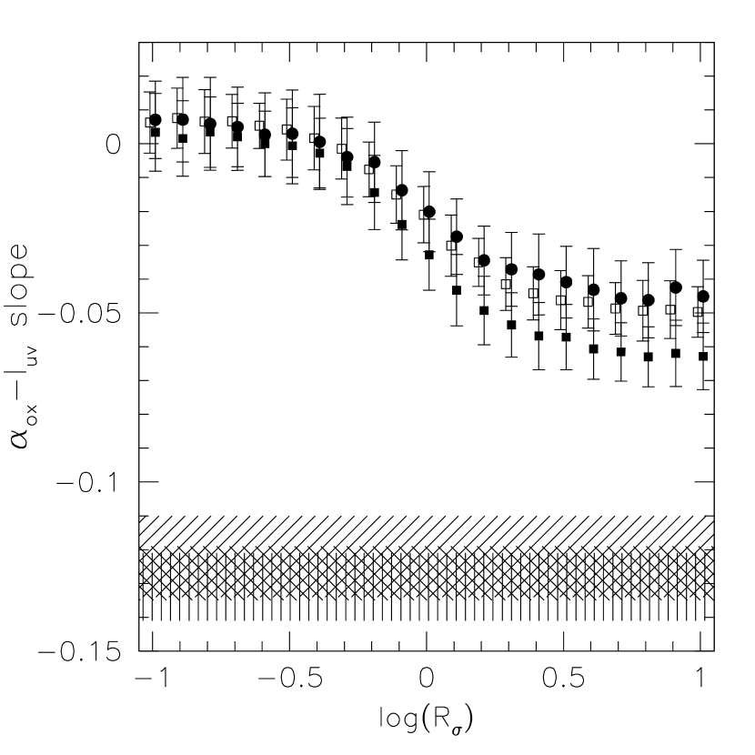
Figure 16.— Slopes of the apparent $\alpha$${}_{\textrm{\scriptsize{ox}}}$-$l_{\textrm{\scriptsize{uv}}}$ anti-correlation (top) and the $l_{\textrm{\scriptsize{x}}}$-$l_{\textrm{\scriptsize{uv}}}$ correlation (bottom) as a function of the optical/UV-to-X-ray dispersion ratio, $R$${}_{\textrm{\scriptsize{$\sigma$}}}$, from simulated samples similar to the main SDSS sample (solid circles), the main$+$high-$z$ samples (solid squares), and the combined sample (open squares). Each point represents the average slope obtained from 100 simulated samples, equally spaced in $\log$($R$${}_{\textrm{\scriptsize{$\sigma$}}}$); the squares have been displaced by $\pm$0.01 from the true $\log$($R$${}_{\textrm{\scriptsize{$\sigma$}}}$) values for clarity. The hatched regions represent the 1$\sigma$ ranges measured in the main SDSS sample (right-slanted), the main$+$high-$z$ samples (vertical lines), and the combined sample (left-slanted).

4. Discussion and Conclusions

The SDSS is providing one of the largest optically selected AGN samples to date with substantially better photometry and higher completeness than previous well-studied optical color selected samples like the BQS sample. Various studies have found that the bright $B$ band selection limit ($B<16.16$) and blue $U-B$ cut ($U-B<-0.44$) of the BQS sample bias the sample towards $z<0.5$ and the bluest luminous AGNs, systematically excluding redder objects, while including some AGNs fainter than the quoted magnitude limit (e.g., Wampler & Ponz, 1985; Wisotzki et al., 2000; Jester et al., 2005). SDSS uses 4-dimensional redshift-dependent color selection and flux limits the AGN sample in the i-band (with an effective wavelength of 7481 Å  compared to 4400 Å for the BQS sample’s $B$ band), which, together with the accurate CCD photometry, creates a highly complete, representative sample of optical AGNs.

We have selected a representative sample of 155 radio-quiet SDSS AGNs from DR2, serendipitously observed in medium-deep ROSAT pointings, creating an unbiased sample with sensitive coverage in the rest-frame UV, 20 cm radio, and soft X-ray bands. Using the serendipitous ROSAT observations of SDSS AGNs supplemented by 36 high-redshift luminous QSOs and 37 Seyfert 1 galaxies, we consider the relations between rest-frame UV (measured at 2500 Å) and X-ray (at 2 keV) emission in a combined sample of 228 AGNs with an X-ray detection fraction of $86$%. We have carefully dealt with a variety of selection and analysis issues, ranging from the appropriateness of the sample to the suitability of the statistical methods. The removal of RL and BAL AGNs is essential if we want to study the intrinsic relations between UV and X-ray energy generation in the typical luminous AGN, as it restricts the confusing effects of jet emission and X-ray absorption. To the extent that we can measure them, BAL AGNs have the same underlying X-ray emission properties as normal RQ AGNs (e.g., Gallagher et al., 2002), but they remain hidden by strong absorption. Consequently we take special care to remove all known BALs from our sample and to consider the effects of unidentified BAL AGNs in specific redshift ranges.

We find that the monochromatic luminosity at 2500 Å and 2 keV are correlated (at the 11.5$\sigma$ level), independent of their strong correlations with redshift. This correlation cannot be caused by the steep fall-off of the bright AGN number-density combined with a large ratio of optical/UV-to-X-ray dispersion in our sample as suggested by C83, F95, YSB98, and Yuan (1999). We take special care when evaluating the statistical significance of partial correlations in censored datasets. Using the partial Kendall’s $\tau_{12,3}$ and the EM linear regression method in an optically selected sample with a wide range of AGN luminosities and redshifts and a large X-ray detection fraction, we can properly assess the significance and estimate the parameters of the correlations. In addition, we use Monte Carlo realizations of mock relations in simulated samples to establish the applicability of the above methods. We confirm that the slope of the $l_{\textrm{\scriptsize{x}}}$–$l_{\textrm{\scriptsize{uv}}}$ correlation is less than one ($\sim$0.65), implying a dependence of the optical/UV-to-X-ray index, $\alpha$${}_{\textrm{\scriptsize{ox}}}$, on monochromatic luminosity and/or redshift. We find that $\alpha$${}_{\textrm{\scriptsize{ox}}}$ is primarily dependent on rest-frame monochromatic UV luminosity (at the 7.4–10.6$\sigma$ level), while any redshift dependence is insignificant ($\lesssim 1.1\sigma$).

The $\alpha$${}_{\textrm{\scriptsize{ox}}}$–$l$${}_{\textrm{\scriptsize{uv}}}$ anti-correlation implies that AGNs redistribute their energy in the UV and X-ray bands depending on overall luminosity, with more luminous AGNs emitting fewer X-rays per unit UV luminosity than less luminous AGNs. Currently, no self-consistent theoretical study is able to explain from first principles why $\alpha$${}_{\textrm{\scriptsize{ox}}}$ should be in the observed range, much less predict its variation with $l$${}_{\textrm{\scriptsize{uv}}}$. Theoretical studies of Shakura & Sunyaev (1973) disks give predictions of the rest-frame UV emission but cannot predict the X-ray emission, which is believed to originate in a hot coronal gas of unknown geometry and disk-covering fraction. Recent advances in magnetohydrodynamic simulations of accretion disks (e.g., Balbus & Hawley, 1998, and references therein) offer the promise of a self-consistent disk$+$corona model of AGN emission. In such a model, the dissipation of magnetic fields, arising from the magneto-rotational instability deep in the accretion disk, could heat the coronal gas to X-ray emitting temperatures (J. H. Krolik 2004, private communication; see also Krolik, 1999). Our empirical relation between rest-frame UV and soft-X-ray emission in AGNs and the $\alpha_{\textrm{\scriptsize{ox}}}$–$l$${}_{\textrm{\scriptsize{uv}}}$ anti-correlation provide the best constraints yet that future self-consistent disk$+$corona models must explain.

The observed lack of redshift dependence of $\alpha$${}_{\textrm{\scriptsize{ox}}}$ at fixed luminosity provides evidence for the remarkable constancy of the accretion process in the immediate vicinity of the black hole, despite the dramatic changes of AGN hosts and the strong evolution of AGN number densities over the history of the Universe. The sample used here provides no evidence for non-linearities in the $\alpha$${}_{\textrm{\scriptsize{ox}}}$–$l$${}_{\textrm{\scriptsize{uv}}}$ relation. The dispersions observed around the $l_{\textrm{\scriptsize{x}}}$–$l_{\textrm{\scriptsize{uv}}}$ and $\alpha$${}_{\textrm{\scriptsize{ox}}}$–$l_{\textrm{\scriptsize{uv}}}$ relations cannot be accounted for by measurement errors and AGN variability alone, suggesting that black-hole mass, accretion rate, and/or spin (and the corresponding differences in accretion modes, energy generation mechanisms, and feedback) could be contributing to the observed dispersion.

Our results are qualitatively consistent with previous studies (e.g., Avni & Tananbaum, 1986; Vignali, Brandt, & Schneider, 2003), but the new results are quantitatively better since they are based on a large, highly complete sample with medium-deep soft X-ray coverage and carefully controlled systematic biases. Although larger samples of optically selected AGNs with X-ray coverage can be constructed (e.g., Wilkes et al., 1994; Green et al., 1995; Anderson et al., 2003), the existing survival analysis tools cannot guarantee an accurate recovery of the intrinsic rest-frame UV to X-ray relations based on pattern censored data with shallow X-ray coverage and low X-ray detection fraction. Stacking analysis can be used on optical AGNs with shallow X-ray coverage (e.g., Green et al., 1995), but this method provides only mean values, without constraining the spread in each bin. In addition, stacking analyses done to date have not always allowed for binning in Galactic Hydrogen column densities, redshifts, radio-loudness, and strong UV-absorption. The $l_{\textrm{\scriptsize{x}}}$–$l_{\textrm{\scriptsize{uv}}}$ relation presented here can be used to predict more accurately the intrinsic X-ray fluxes of AGNs with known optical/UV luminosity and serves to define the “normal” range of soft X-ray emission for a typical AGN (i.e., RQ, non-BAL AGNs, unaffected by absorption). Based on this definition of normal X-ray emission, it is easier to determine if a “special” class of AGNs differs in its X-ray properties from normal AGNs. X-ray “weak” AGNs are an example of such a special AGN class. Risaliti et al. (2003) used the BQS sample to define normal AGNs, and suggested that some AGNs in the Hamburg Quasar Survey (HQS, Hagen et al., 1995) are X-ray weaker in comparison. However, Brandt, Schneider, & Vignali (2004) caution that since the HQS AGNs are among the most luminous objects in the rest-frame UV, the observed steep $\alpha$${}_{\textrm{\scriptsize{ox}}}$ values are expected based on the $\alpha$${}_{\textrm{\scriptsize{ox}}}$–$l_{\textrm{\scriptsize{uv}}}$ anti-correlation for about half of the objects (see their Figure 3). Our more accurate prediction of the optical/UV-to-X-ray emission of normal AGN will also allow researchers to constrain the X-ray emission associated with jets in RL AGNs (assuming that AGN jets do not contribute to the emission at 2500 Å, but see Baker & Hunstead, 1995; Baker et al., 1995; Cheung, 2002) and to study the X-ray properties of other special AGNs; e.g, red AGNs, AGNs without emission lines, or AGNs with unusual emission lines (e.g., Gallagher et al., 2005). The $\alpha$${}_{\textrm{\scriptsize{ox}}}$–$l$${}_{\textrm{\scriptsize{uv}}}$ relation of normal AGNs presented in this paper can also lead to more accurate estimates of the bolometric luminosities of AGNs, resulting in tighter constraints on the importance of AGN-phase mass accretion for the growth of supermassive black holes as described in, e.g., Marconi et al. (2004). Assuming the Elvis et al. (1994) spectral energy distribution (SED) and $-1.7<\alpha_{\textrm{\scriptsize{ox}}}<-1.26$ (where the majority of our optically selected RQ non-absorbed AGNs lie; see Figure 11) together with the $\alpha$${}_{\textrm{\scriptsize{ox}}}$–$l$${}_{\textrm{\scriptsize{uv}}}$ relation from Eqn. 6, we estimate that the ratio of the 0.5–2.0 keV luminosity to the bolometric luminosity varies by a factor of 6–9 over the luminosity range $l_{\textrm{\scriptsize{uv}}}=28.5-31.8$ (depending on the inclusion or exclusion of the infrared bump in the computation of the bolometric luminosity). If neglected, the variation of the bolometric correction with AGN luminosity could lead to substantial systematic errors in bolometric luminosity estimates.

Future SDSS data releases will allow the enlargement of the optical/UV/soft-X-ray sample of AGNs, as well as provide large new samples of optically selected AGNs serendipitously observed with XMM-Newton and Chandra, as the sky-coverage of X-ray satellites increases with time. Larger samples will include more homogeneous low-luminosity AGN data, providing more sensitive constraints on the non-linearity of the $\alpha$${}_{\textrm{\scriptsize{ox}}}$–$l_{\textrm{\scriptsize{uv}}}$ relation. In addition, longer-wavelength optical/UV monochromatic flux estimates would complement the rest-frame UV measurements at 2500 Å used here, to minimize any effects of dust absorption in the UV on the $l_{\textrm{\scriptsize{x}}}$–$l_{\textrm{\scriptsize{uv}}}$ relation (e.g., Gaskell et al., 2003, but see also Hopkins et al. 2004). The extension to samples observed in harder X-ray bands is also necessary to constrain the possible effects of soft-X-ray absorption better. This can be achieved by considering an $\alpha$${}_{\textrm{\scriptsize{ox}}}$ index computed using rest-frame $\approx$5 keV instead of 2 keV X-ray monochromatic fluxes.

Hasinger (2004) reports that X-ray selected AGN samples have $l_{\textrm{\scriptsize{x}}}$–$l_{\textrm{\scriptsize{uv}}}$ correlations consistent with a slope of one and no $\alpha$${}_{\textrm{\scriptsize{ox}}}$ dependence on either luminosity or redshift. Current X-ray selected samples with optical identifications are large and cover wide ranges of optical/UV and X-ray luminosity, but they seldom constrain the optical/UV absorption, radio loudness, or host-galaxy contribution of the sources. In addition, some X-ray selected samples are biased toward particular optical AGN types (e.g., narrow-line Seyfert 1s in bright soft X-ray samples; Grupe et al., 2004) and could contain a larger fraction of absorbed AGNs. More studies are necessary to reconcile the results obtained for optically color-selected and X-ray selected samples, taking into account the sample selection effects in flux limited samples introduced by the optical/UV and X-ray AGN population number density and luminosity evolution with cosmic time.

Firmly establishing the correlation between rest-frame UV and X-ray emission in AGNs is the first step toward understanding their generation mechanisms and interrelations. A reasonable next step is to try to relate the correlations found here to reasonable estimates of black-hole masses and accretion rates. The difficulty in this endeavor lies in the fact that direct black-hole mass measurements and bolometric luminosity estimates are not available for large AGN samples like those considered here. Indirect black-hole mass measurements can be obtained from a combination of monochromatic luminosity and broad emission-line width measurements as shown for BQS sample AGNs by Kaspi et al. (2000) and SDSS AGNs by McLure & Dunlop (2004). Such estimates, however, will depend on the extrapolation of Kaspi et al. (2000) relation from lower ($\lambda L_{\lambda}(5100\,\textrm{\AA})\lesssim 2\times 10^{45}$, corresponding to $l_{\textrm{\scriptsize{uv}}}\lesssim 30.3$) to higher ($\lambda L_{\lambda}(5100\,\textrm{\AA})\gtrsim 2\times 10^{45}$) luminosity AGNs, the use of different emission lines at different redshifts (e.g., H$\beta$ and Mg II for the SDSS sample presented here), as well as a non-trivial correction for the effects of the host-galaxy, giving rise to possible systematic errors. We are currently investigating the feasibility of this endeavor for the SDSS sample presented here.

Acknowledgments

We thank M. Akritas for fruitful discussions on the suitability of the statistical methods used in the paper and P. Hall and J. R. Trump for help with the BAL classification of SDSS AGNs. The authors acknowledge the help of W. Yuan in implementing his work on the slope validation of the $l_{\textrm{\scriptsize{x}}}$–$l_{\textrm{\scriptsize{uv}}}$ correlation and the help of David Schlegel with SDSS spectroscopy. We are grateful to Gordon Richards, Sebastian Jester and Sarah Gallagher, as well as an anonymous referee, for helping us to improve this manuscript. IVS, WNB, and DPS acknowledge the support of NASA LTSA grant NAG5-13035 and the CXC grant GO2-3134X. CV acknowledges the support of MIUR COFIN grant 03-02-23.

Funding for the Sloan Digital Sky Survey (SDSS) has been provided by the Alfred P. Sloan Foundation, the Participating Institutions, the National Aeronautics and Space Administration, the National Science Foundation, the U.S. Department of Energy, the Japanese Monbukagakusho, and the Max Planck Society. The SDSS Web site is http://www.sdss.org/. The SDSS is managed by the Astrophysical Research Consortium (ARC) for the Participating Institutions. The Participating Institutions are The University of Chicago, Fermilab, the Institute for Advanced Study, the Japan Participation Group, The Johns Hopkins University, Los Alamos National Laboratory, the Max-Planck-Institute for Astronomy (MPIA), the Max-Planck-Institute for Astrophysics (MPA), New Mexico State University, University of Pittsburgh, Princeton University, the United States Naval Observatory, and the University of Washington.

This research has made use of the NASA/IPAC Extragalactic Database (NED) which is operated by the Jet Propulsion Laboratory, California Institute of Technology, under contract with the National Aeronautics and Space Administration.

Table 1SDSS-ROSAT AGN data

SDSS ID	$z$	Obs. ID	$T$${}_{\textrm{\scriptsize{exp}}}$	$\delta$	Cnt	$f$${}_{\textrm{\scriptsize{2500}}}$	$f$${}_{\textrm{\scriptsize{x}}}$	$f$${}_{\textrm{\scriptsize{2{keV}}}}$	$\alpha_{\textrm{\scriptsize{ox}}}$	$l$${}_{\textrm{\scriptsize{x}}}$	$l$${}_{\textrm{\scriptsize{uv}}}$	i	$\Delta(g-i)$	Flag
(1)	(2)	(3)	(4)	(5)	(6)	(7)	(8)	(9)	(10)	(11)	(12)	(13)	(14)	(15)
SDSSJ012602.21$-$001924.1	1.7659	rp800645n00	12.0	11	19.0	$-$3.71	$-$13.70	$-$8.08	$-$1.68	26.80	31.17	17.94	$+$0.144	1
SDSSJ021000.72$-$100358.0	1.9604	rp800114n00	13.8	9	72.0	$-$4.16	$-$13.20	$-$7.56	$-$1.30	27.41	30.81	19.23	$-$0.180	1
SDSSJ022225.49$-$090258.5	0.2242	rp800016n00	11.6	14	5.6	$-$4.28	$-$13.91	$-$8.65	$-$1.68	24.41	28.78	18.49	$-$0.033	0
SDSSJ022226.11$-$085701.3	0.1667	rp800016n00	11.5	15	445.4	$-$4.17	$-$12.32	$-$7.08	$-$1.12	25.72	28.63	17.85	$+$0.193	1
SDSSJ022356.30$-$085707.8	1.5762	rp800016n00	12.5	10	13.0	$-$4.13	$-$13.92	$-$8.34	$-$1.62	26.45	30.67	18.90	$+$0.220	1
SDSSJ022435.93$-$090001.3	1.6118	rp800016n00	9.2	19	15.1	$-$4.12	$-$13.62	$-$8.03	$-$1.50	26.78	30.69	19.11	$-$0.015	1
SDSSJ023305.95$+$003856.4	0.2441	rp800482n00	26.1	11	107.0	$-$5.13	$-$13.31	$-$8.04	$-$1.12	25.10	28.01	18.52	$+$0.559	1
SDSSJ023306.26$+$004614.5	2.2906	rp800482n00	26.5	9	36.2	$-$4.65	$-$13.82	$-$8.13	$-$1.34	26.96	30.44	20.33	$-$0.159	1
SDSSJ023325.32$+$002914.9	2.0171	rp800482n00	25.1	16	81.1	$-$3.74	$-$13.43	$-$7.77	$-$1.55	27.21	31.24	18.25	$+$0.007	1
SDSSJ023333.24$+$010333.1	2.0587	rp800482n00	19.6	19	5.5	$-$3.72	$-$14.02	$-$8.37	$-$1.78	26.64	31.28	18.30	$-$0.038	0

Note. — The complete version of this table is in the electronic edition of the Journal. The printed edition contains only a sample of ten objects. Note 1: These AGNs were the targets for their respective ROSAT PSPC pointings. Note 2: These AGNs were not detected in the selected ROSAT pointings; X-ray fluxes are from XMM-Newton, Chandra, or shorter ROSAT exposures as specified. The units of luminosity are erg s^-1, of monochromatic luminosity – erg s^-1 Hz^-1. Columns: (1) SDSS ID; (2) redshift; (3) X-ray observation ID; (4) the effective X-ray exposure time, $T$${}_{\textrm{\scriptsize{exp}}}$, in 10³sec; (5) $\delta$, the X-ray source off-axis angle in arcmin; (6) total source counts, corrected for background and aperture size; the precision quoted is higher than the accuracy; (7) $f$${}_{\textrm{\scriptsize{2500}}}$, the logarithm of the 2500 Å monochromatic flux, not band-pass corrected; (8) $f$${}_{\textrm{\scriptsize{x}}}$, the logarithm of the 0.5-2 keV flux, not band-pass corrected; (9) $f$${}_{\textrm{\scriptsize{2{keV}}}}$ the logarithm of the 2 keV monochromatic flux, not band-pass corrected; (10) $\alpha_{\textrm{\scriptsize{ox}}}$, the optical/UV-to-X-ray index; (11) $l$${}_{\textrm{\scriptsize{x}}}$, the logarithm of the 2 keV monochromatic luminosity, band-pass corrected; (12) $l$${}_{\textrm{\scriptsize{uv}}}$, the logarithm of the 2500 Å monochromatic luminosity, band-pass corrected; (13) i, the point source SDSS apparent magnitude, corrected for Galactic extinction; (14) the relative PSF color, $\Delta(g-i)$, corrected for Galactic extinction; (15) this flag is set to 1 if the AGN is X-ray detected.

Table 2X-ray Detection Fractions

Sample	X-ray	Total	% X-ray
	Detected	AGN	Detected
Main	126	155	81%
High-$z$	32	36	89%
Sy 1	37	37	100%
Combined	195	228	86%

Table 3X-ray UV correlations

Relation	Sample	$N$${}_{\textrm{\scriptsize{AGN}}}$	% X-ray	Signi-	$\tau_{\textrm{\scriptsize{12,3}}}$	Regression
			Detected	ficance		Residuals
$l_{\textrm{\scriptsize{2keV}}}$ vs. $l_{\textrm{\scriptsize{2500\,\AA}}}$	M,H,S	228	86%	11.5$\sigma$	0.38	0.36
$l_{\textrm{\scriptsize{2keV}}}$ vs. $l_{\textrm{\scriptsize{2500\,\AA}}}$	M,H	191	83%	8.7$\sigma$	0.30	0.37
$l_{\textrm{\scriptsize{2keV}}}$ vs. $l_{\textrm{\scriptsize{2500\,\AA}}}$	M	155	81%	7.4$\sigma$	0.28	0.39
$\alpha_{\textrm{\scriptsize{ox}}}$ vs. $l_{\textrm{\scriptsize{2500\,\AA}}}$	M,H,S	228	86%	10.6$\sigma$	$-$0.33	0.14
$\alpha_{\textrm{\scriptsize{ox}}}$ vs. $l_{\textrm{\scriptsize{2500\,\AA}}}$	M,H	191	83%	9.2$\sigma$	$-$0.32	0.14
$\alpha_{\textrm{\scriptsize{ox}}}$ vs. $l_{\textrm{\scriptsize{2500\,\AA}}}$	M	155	81%	7.4$\sigma$	$-$0.30	0.15
$\alpha_{\textrm{\scriptsize{ox}}}$ vs. $z$	M,H,S	228	86%	1.1$\sigma$	$+$0.03	…
$\alpha_{\textrm{\scriptsize{ox}}}$ vs. $z$	M,H	191	83%	1.1$\sigma$	$-$0.03	…
$\alpha_{\textrm{\scriptsize{ox}}}$ vs. $z$	M	155	81%	1.0$\sigma$	$-$0.02	…

Note. — Sample M refers to the main SDSS sample, sample H to the high-$z$ sample, and sample S to the Sy 1 sample. All cases test partial correlations, taking into account the effect of a third variable which is either redshift (in the first six cases) or $l_{\textrm{\scriptsize{2500\,\AA}}}$ (in the last three).

References

- Abazajian et al. (2004) Abazajian, K., et al. 2004, AJ, 128, 502
- Abazajian et al. (2005) Abazajian, K., et al. 2005, AJ, submitted, astro-ph/0410239
- Akritas & Siebert (1996) Akritas, M. G. & Siebert, J. 1996, MNRAS, 278, 919
- Anderson (1985) Anderson, S. F. 1985, Ph.D. Thesis, University of Washington
- Anderson & Margon (1987) Anderson, S. F. & Margon, B. 1987, ApJ, 314, 111
- Anderson et al. (2003) Anderson, S. F., et al. 2003, AJ, 126, 2209
- Avni & Tananbaum (1982) Avni, Y. & Tananbaum, H. 1982, ApJ, 262, L17
- Avni & Tananbaum (1986) Avni, Y. & Tananbaum, H. 1986, ApJ, 305, 83
- Baker & Hunstead (1995) Baker, J. C., & Hunstead, R. W. 1995, ApJ, 452, L95
- Baker et al. (1995) Baker, J. C., Hunstead, R. W., & Brinkmann, W. 1995, MNRAS, 277, 553
- Balbus & Hawley (1998) Balbus, S. A. & Hawley, J. F. 1998, Reviews of Modern Physics, 70, 1
- Bechtold et al. (2003) Bechtold, J., et al. 2003, ApJ, 588, 119
- Becker, White, & Helfand (1995) Becker, R. H., White, R. L., & Helfand, D. J. 1995, ApJ, 450, 559
- Brandt, Laor, & Wills (2000) Brandt, W. N., Laor, A., & Wills, B. J. 2000, ApJ, 528, 637
- Brandt, Schneider, & Vignali (2004) Brandt, W., Schneider, D., & Vignali, C. 2004, AGN Physics with the Sloan Digital Sky Survey, Proceedings of a conference held in Princeton, NJ, USA, 27-31 July 2003, edited by G. T. Richards and P. B. Hall, ASP Conference Series, Volume 311. San Francisco: Astronomical Society of the Pacific, 2004, p.303
- Broos et al. (2004) Broos, P., Townsley, L., Getman, K., & Bauer, F. 2004, “ACIS Extract, An ACIS Point Source Extraction Package”, http://www.astro.psu.edu/xray/docs/TARA/ae_users_guide.html
- Chanan (1983) Chanan, G. A. 1983, ApJ, 275, 45
- Cheung (2002) Cheung, C. C. 2002, ApJ, 581, L15
- Condon et al. (1998) Condon, J. J., Cotton, W. D., Greisen, E. W., Yin, Q. F., Perley, R. A., Taylor, G. B., & Broderick, J. J. 1998, AJ, 115, 1693
- Croom et al. (2001) Croom, S. M., Smith, R. J., Boyle, B. J., Shanks, T., Loaring, N. S., Miller, L., & Lewis, I. J. 2001, MNRAS, 322, L29
- Djorgovski et al. (1998) Djorgovski, S. G., Gal, R. R., Odewahn, S. C., de Carvalho, R. R., Brunner, R., Longo, G., & Scaramella, R. 1998, Wide Field Surveys in Cosmology, 14th IAP meeting held May 26-30, 1998, Paris. Publisher: Editions Frontieres, p. 89
- Elvis et al. (1994) Elvis, M., et al. 1994, ApJS, 95, 1
- Feigelson & Nelson (1985) Feigelson, E. D. & Nelson, P. I. 1985, ApJ, 293, 192
- Fiore et al. (1998) Fiore, F., Laor, A., Elvis, M., Nicastro, F., & Giallongo, E. 1998, ApJ, 503, 607
- Foltz et al. (1990) Foltz, C. B., Chaffee, F. H., Hewett, P. C., Weymann, R. J., & Morris, S. L. 1990, BAAS, 22, 806
- Gallagher et al. (2002) Gallagher, S. C., Brandt, W. N., Chartas, G., & Garmire, G. P. 2002, ApJ, 567, 37
- Gallagher et al. (2005) Gallagher, S. C., Richards G. T., Hall, P. B. et al. 2005, AJ, in press, astro-ph/0410641
- Gallo et al. (2004) Gallo, L. C., Boller, T., Brandt, W. N., Fabian, A. C., & Vaughan, S. 2004, A&A, 417, 29
- Garmire et al. (2003) Garmire, G. P., Bautz, M. W., Ford, P. G., Nousek, J. A., & Ricker, G. R. 2003, Proc. SPIE, 4851, 28
- Gaskell et al. (2003) Gaskell C. M., Goosmann, R. W., Antonucci R. J., & Whysong, D. H. 2003, ApJ, 616, 147
- Green, McHardy, & Lehto (1993) Green, A. R., McHardy, I. M., & Lehto, H. J. 1993, MNRAS, 265, 664
- Green et al. (1995) Green, P. J., et al. 1995, ApJ, 450, 51
- Grupe, Thomas, & Beuermann (2001) Grupe, D., Thomas, H.-C., & Beuermann, K. 2001, A&A, 367, 470
- Grupe et al. (2004) Grupe, D., Wills, B. J., Leighly, K. M., & Meusinger, H. 2004, AJ, 127, 156
- Hagen et al. (1995) Hagen, H.-J., Groote, D., Engels, D., & Reimers, D. 1995, A&AS, 111, 195
- Hasinger (2004) Hasinger, G., 2004, in Merloni A., Nayakshin S., Sunyaev R., eds, Growing Black Holes: Accretion in a Cosmological Context. Springer-Verlag, Berlin, in press
- Hewett & Foltz (2003) Hewett, P. C. & Foltz, C. B. 2003, AJ, 125, 1784
- Hopkins et al. (2004) Hopkins, P. F., et al. 2004, AJ, 128, 1112
- Irwin, McMahon, & Hazard (1991) Irwin, M., McMahon, R. G., & Hazard, C. 1991, ASP Conf. Ser. 21: The Space Distribution of Quasars, 117
- Isobe, Feigelson, & Nelson (1985) Isobe, T., Feigelson, E. D., & Nelson, P. I. 1985, BAAS, 17, 573
- Isobe, Feigelson, & Nelson (1986) Isobe, T., Feigelson, E. D., & Nelson, P. I. 1986, ApJ, 306, 490
- Ivezić et al. (2002) Ivezić, Ž., et al. 2002, AJ, 124, 2364
- Ivezić et al. (2004) Ivezic, Z., Lupton, R. H., Juric, M., et al. 2004, to appear in ”Proceedings IAU Symposium 222: The Interplay among Black Holes, Stars and ISM in Galactic Nuclei”, edited by T. S. Bergmann, L. C. Ho, & H. R. Schmitt, Cambridge University Press, astro-ph/0404487
- Jansen et al. (2001) Jansen, F., et al. 2001, A&A, 365, L1
- Jester et al. (2005) Jester, S., et al. 2005, AJ, submitted
- Kaspi et al. (2000) Kaspi, S., Smith, P. S., Netzer, H., Maoz, D., Jannuzi, B. T., & Giveon, U. 2000, ApJ, 533, 631
- Kolman et al. (1993) Kolman, M., Halpern, J. P., Martin, C., Awaki, H., & Koyama, K. 1993, ApJ, 403, 592
- Kriss & Canizares (1985) Kriss, G. A. & Canizares, C. R. 1985, ApJ, 297, 177
- Krolik (1999) Krolik, J. H. 1999, “Active galactic nuclei: from the central black hole to the galactic environment”, Princeton University Press
- La Franca et al. (1995) La Franca, F., Franceschini, A., Cristiani, S., & Vio, R. 1995, A&A, 299, 19
- LaValley, Isobe, & Feigelson (1992) Lavalley, M., Isobe, T., & Feigelson, E. 1992, ASP Conf. Ser. 25: Astronomical Data Analysis Software and Systems I, 1, 245
- Marconi et al. (2004) Marconi, A., Risaliti, G., Gilli, R., Hunt, L. K., Maiolino, R., & Salvati, M. 2004, MNRAS, 351, 169
- Markowitz, Edelson, & Vaughan (2003) Markowitz, A., Edelson, R., & Vaughan, S. 2003, ApJ, 598, 935
- McLure & Dunlop (2004) McLure, R. J. & Dunlop, J. S. 2004, MNRAS, 352, 1390
- Menou et al. (2001) Menou, K., et al. 2001, ApJ, 561, 645
- Nandra et al. (1997) Nandra, K., George, I. M., Mushotzky, R. F., Turner, T. J., & Yaqoob, T. 1997, ApJ, 476, 70
- Nandy et al. (1975) Nandy, K., Thompson, G. I., Jamar, C., Monfils, A., & Wilson, R. 1975, A&A, 44, 195
- Natali et al. (1998) Natali, F., Giallongo, E., Cristiani, S., & La Franca, F. 1998, AJ, 115, 397
- Oke & Gunn (1983) Oke, J. B. & Gunn, J. E. 1983, ApJ, 266, 713
- Page et al. (2003) Page, K. L., Turner, M. J. L., Reeves, J. N., O’Brien, P. T., & Sembay, S. 2003, MNRAS, 338, 1004
- Pfeffermann et al. (1987) Pfeffermann, E., et al. 1987, Proc. SPIE, 733, 519
- Richards et al. (2002) Richards, G. T., et al. 2002, AJ, 123, 2945
- Richards et al. (2003a) Richards, G. T., et al. 2003, AJ, 126, 1131
- Reichard et al. (2003b) Reichard, T. A., et al. 2003, AJ, 126, 2594
- Richards et al. (2005) Richards, G. T., et al. 2005, in preparation
- Richstone & Schmidt (1980) Richstone, D. O. & Schmidt, M. 1980, ApJ, 235, 361
- Risaliti et al. (2003) Risaliti, G., Elvis, M., Gilli, R., & Salvati, M. 2003, ApJ, 587, L9
- Schlegel, Finkbeiner, & Davis (1998) Schlegel, D. J., Finkbeiner, D. P., & Davis, M. 1998, ApJ, 500, 525
- Schneider et al. (2001) Schneider, D. P., et al. 2001, AJ, 121, 1232
- Schneider et al. (2003) Schneider, D. P., et al. 2003, AJ, 126, 2579
- Shakura & Sunyaev (1973) Shakura, N. I. & Sunyaev, R. A. 1973, A&A, 24, 337
- Schmidt & Green (1983) Schmidt, M., & Green, R. F. 1983, ApJ, 269, 352
- Spergel et al. (2003) Spergel, D. N., et al. 2003, ApJS, 148, 175
- Stark et al. (1992) Stark, A. A., Gammie, C. F., Wilson, R. W., Bally, J., Linke, R. A., Heiles, C., & Hurwitz, M. 1992, ApJS, 79, 77
- Stoughton et al. (2002) Stoughton, C., et al. 2002, AJ, 123, 485
- Strüder et al. (2001) Strüder, L., et al. 2001, A&A, 365, L18
- Tananbaum et al. (1979) Tananbaum, H., et al. 1979, ApJ, 234, L9
- Tolea, Krolik, & Tsvetanov (2002) Tolea, A., Krolik, J. H., & Tsvetanov, Z. 2002, ApJ, 578, L31
- Uttley & McHardy (2004) Uttley, P. & McHardy, I. M. 2004, Progress of Theoretical Physics, in press (astro-ph/0402407)
- Uttley, McHardy, & Papadakis (2002) Uttley, P., McHardy, I. M., & Papadakis, I. E. 2002, MNRAS, 332, 231
- Vanden Berk et al. (2001) Vanden Berk, D. E., et al. 2001, AJ, 122, 549
- Vanden Berk et al. (2004a) Vanden Berk, D. E., et al. 2004, ApJ, 601, 692
- Vanden Berk et al. (2005) Vanden Berk, D. E., et al. 2005, AJ, in press
- Vignali et al. (2003) Vignali, C., et al. 2003, AJ, 125, 2876
- Vignali, Brandt, & Schneider (2003) Vignali, C., Brandt, W. N., & Schneider, D. P. 2003, AJ, 125, 433
- Walter & Fink (1993) Walter, R. & Fink, H. H. 1993, A&A, 274, 105
- Wampler & Ponz (1985) Wampler, E. J. & Ponz, D. 1985, ApJ, 298, 448
- Watson et al. (2003) Watson, M. G., et al. 2003, Astronomische Nachrichten, 324, 89
- Weymann et al. (1991) Weymann, R. J., Morris, S. L., Foltz, C. B., & Hewett, P. C. 1991, ApJ, 373, 23
- White et al. (1994) White, N. E., Giommi, P., & Angelini, L. 1994, Bulletin of the American Astronomical Society, 26, 1372
- Wilkes et al. (1994) Wilkes, B. J., Tananbaum, H., Worrall, D. M., Avni, Y., Oey, M. S., & Flanagan, J. 1994, ApJS, 92, 53
- Wisotzki et al. (2000) Wisotzki, L., Christlieb, N., Bade, N., Beckmann, V., Köhler, T., Vanelle, C., & Reimers, D. 2000, A&A, 358, 77
- Worrall et al. (1987) Worrall, D. M., Tananbaum, H., Giommi, P., & Zamorani, G. 1987, ApJ, 313, 596
- Yip et al. (2004a) Yip, C. W., et al. 2004, AJ, 128, 585
- Yip et al. (2004b) Yip, C. W., et al. 2004, AJ, 128, 2603
- York et al. (2000) York, D. G., et al. 2000, AJ, 120, 1579
- Yuan, Siebert, & Brinkmann (1998) Yuan, W., Siebert, J., & Brinkmann, W. 1998, A&A, 334, 498
- Yuan (1999) Yuan, W., 1999, “Japan-Germany Workshop on AGN and the X-ray Background”, edited by T. Takahashi & H. Inoue
- Zamorani et al. (1981) Zamorani, G., et al. 1981, ApJ, 245, 357