A search for Warm-Hot Intergalactic Medium features in the X-ray spectra of Mkn 421 with the XMM-Newton RGS

We present the high-resolution X-ray spectra of Mkn 421 obtained in November 2003 with the RGS aboard the XMM-Newton satellite. This Target of Opportunity observation was triggered because the source was in a high state of activity in the X-ray band. These data are compared with three archival RGS observations of the same source performed in November and December 2002 and one in June 2003. We searched for the presence of absorption features due to warm-hot intergalactic medium (WHIM). We identify various spectral features, most of which are of instrumental origin. With the sensitivity provided by our spectra we were able to identify only two lines of astronomical origin, namely features at $23.5$ Å, probably due to interstellar neutral oxygen absorption, and at $21.6$ Å, which corresponds to a zero-redshift OVII K$\alpha$ transition. For the latter, we derive an upper limit to the gas temperature, which is consistent with WHIM, of a few times $10^{5}$ K, if the gas density has a value of $n_{e}\gtrsim 10^{-5}$ cm^-3.

1 Introduction

The baryon density at $z>2$ calculated from observations of hydrogen and helium absorption lines in the Ly$\alpha$ forest (Rauch et al. 1997) is in good agreement with standard Big–Bang nucleosynthesis predictions (Burles & Tyler 1998). This is not true at lower redshifts: at $z\sim 0$, all current analyses indicate that, after adding the well–observed contributions, the local baryon density is $\Omega_{bar,obs}\sim 0.007$ (see e.g. Fukugita, Hogan & Peebles 1997), much lower than the predicted value $\Omega_{bar,n-syn}\sim 0.035-0.04$ (Burles & Tytler 1998).
High–resolution, large–scale hydrodynamic simulations of galaxy formation have been used to predict the baryon distribution at the present epoch and at moderate redshift. The main result of such simulations is that approximately 30%–40% of the baryons in the present–day universe should reside in a Warm–Hot Intergalactic Medium (WHIM), shock–heated to temperatures of $10^{5}-10^{7}$ K. Most of these warm–hot baryons seem to reside in diffuse filamentary large–scale structures with overdensities of 10–30 and not in virialized objects such as galaxy groups (Cen & Ostriker 1999; Davé et al. 2001).
Numerical simulations have demonstrated that H–like and He–like ions of the heavy elements composing the WHIM can give rise to absorption lines in the soft X–ray spectra of background sources. OVII, OVIII and NeIX should dominate the relative abundance distributions of collisionally ionized and photoionized+collisionally ionized gas over a broad range of temperatures ($5\times 10^{5}$–$10^{7}$ K, Nicastro et al. 1999), where the WHIM distribution peaks (Davé et al. 2001; Fang & Canizares 2000). Absorption lines at 21.6 Å, 18.97 Å  and 13.4 Å, respectively, should then be observable in the soft X–ray spectra of strong background sources (see e.g. Aldcroft et al. 1994; Hellsten, Gnedin & Miralda–Escudé 1998; Perna & Loeb 1998; Fang & Canizares 2000).
Absorption lines such as the doublet of OVI (1032 Å  and 1038 Å) should be detectable also in the optical–UV band (Mulchaey et al. 1996; Cen et al. 2001), for temperatures of $1-5\times 10^{5}$ K, tracing the low–temperature tail of the WHIM distribution. Current far–UV observations have proved the existence of such a low–temperature component with the detection of OVI absorption lines up to $z\sim 0.2$ (e.g. Sembach et al. 2000; Tripp et al. 2001).
Soft X–ray spectra provide an even better opportunity than the UV spectra: the detection and the study of these components is needed for the proper understanding of large and small–scale structures in the Universe, providing independent constraints on cosmological parameters.
The predicted highly ionized gas, however, has been poorly studied so far, because of instrumental limitations. New spectrometers aboard Chandra (HRCS/LETG) and XMM–Newton (RGS) have increased the sensitivity and the resolution of the X–ray observatories slightly beyond the WHIM detection limit. At present, only the strongest of these systems (EW $>10$ mÅ) have been detected against the spectra of very bright background sources (Nicastro et al. 2002; Mathur, Weimberg & Chen 2002; Fang et al. 2002; Fang, Sembach & Canizares 2003; Cagnoni et al. 2004; Nicastro 2003). Furthermore, only two of them were identified as signatures of the WHIM outside the Local Group: an absorbing system at $z\sim 0.05$ toward 3C 273 (Fang et al. 2002) and one at $z\sim 0.01$ toward Mkn 421 (Cagnoni et al. 2002; Nicastro et al. 2003).
High–resolution observations of Mkn 421 have already been performed with Chandra (Nicastro et al. 2001; Nicastro 2003) and with XMM–Newton (Cagnoni 2001; de Vries et al. 2003). The [18–24] Å  spectrum of Mkn 421 changed during the two Chandra observations of 2000. In one, the source was very bright and no absorption or emission lines were detected. In the other, negative and positive residuals from the best–fit power–law model were observed. Nicastro et al. (2001) tentatively identified two different absorbing/emitting systems and proposed that they are intrinsic to the nuclear environments, becoming fully ionized - and thus transparent - as the source brightens.
Further Chandra observations, performed while the source was in a very bright phase, allowed Nicastro (2003) to claim the presence of three absorbing systems located at $z\sim 0$, $z\sim 0.011$ and at $z\sim 0.03$, respectively. The first was identified as the WHIM inside the Local Group, while the last was explained as Mkn 421 intrinsic absorption. The system st $z\sim 0.011$, was interpreted as the WHIM outside the Local Group.
Even the RGS spectrum of Cagnoni (2001) showed two absorbing systems, one inside the Local Group and one at $z\sim 0.01$, contributing an OVII K$\alpha$ absorption line at $\sim 21.8$ Å. de Vries et al. (2003), instead, concentrated on the [22–24] Å  range of the RGS data and found evidence for a 23.5 Å  interstellar neutral Oxygen (1s–2p) absorption feature. Furthermore, they showed a feature at 22.77 Å, which they argued to be a non–Galactic OVI blend.
In this paper we present the results of a XMM–Newton RGS observation of Mkn 421 performed as part of a Target of Opportunity (ToO) program to observe Blazars in high state of activity (see Tagliaferri et al. 2001). We triggered the pointing because the All Sky Monitor aboard Rossi XTE had been reporting high X–ray fluxes from Mkn 421 for several days. We compared our observations with 3 archival RGS spectra of Mkn 421 taken in November and Dicember 2002 and with one taken in June 2003, as part of two different calibration campaigns.

XMM-Newton RGS
Revolution	Obs. Id.	Start time		Total exposurea	Net exposure
		Day	Hour	($10^{4}$ s)	($10^{4}$ s)
0532	0136540301	04/11/2002	00:44:59	2.3	2.1
0532	0136540401	04/11/2002	07:41:43	2.3	2.1
0546	0136541001	01/12/2002	22:59:25	7.1	5.8
0637	0158970101	01/06/2003	12:48:50	4.3	3.0
0720	0150498701	14/11/2003	16:14:04	5.7	4.7

Table 1: Log of the XMM–Newton RGS observations of Mkn 421 taken in 2002 and 2003 that were used during this analysis. A further observation of Mkn421 0537_0136540701 was also performed during the cooling of RGS1 which we have not used. ^a: total amount of Good Time Intervals. ^b: the reprocessing of these data failed; we exclude them from further analysis.

In the following sections, we briefly describe the observations and show the results of the spectral analysis performed on the whole RGS energy range. Then we concentrate on smaller energy ranges, looking carefully for the presence of absorption features whose reality is checked in two ways: first, by comparing the Mkn 421 spectra with the smooth X-ray spectrum of the Crab nebula and second, by paying particular attention to the raw data to check for instrumental effects. Occasional hot or cool pixels are routine in CCD data as a result of cosmic–ray damage and other effects and are treated as part of normal data analysis procedures. Such defects are usually confined to single pixels and are thus significantly narrower than the instrumental line response that is principally caused by scattering from the gratings. Finally, we discuss the results proposing an identification for the possible non–Galactic absorption lines.

2 The XMM–Newton observations and data reduction

The XMM–Newton X–ray payload consists of three Wolter type–1 telescopes, equipped with 3 CCD cameras for X–ray imaging, moderate resolution spectroscopy and photometry (EPIC). Two of these telescopes (those carrying the MOS cameras) are also provided with high resolution Reflection Grating Spectrometers (RGS–1 & RGS–2), operating in the range [0.33–2.5] keV (5–38 Å). Each RGS unit deflects half of its telescope beam, dispersing the striking X–ray light at a wavelength–dependent angle, thus providing a spectral resolution of $E/\Delta E\sim 100-500$ (FWHM). After the launch, however, failures in the read–out electronics of the CCD–7 (RGS–1) and CCD–4 (RGS–2), covering the [10.5–14] Å  and the [20.1–23.9] Å  ranges, respectively, reduced by a factor of 2 the RGS effective area at these wavelengths.
Mkn 421 was the target of a RGS calibration campaign in November and December 2002, aimed at improving the instrumental performances by lowering the operating temperature. The benefits of the cooling manifested as a dramatic reduction of hot columns and flickering pixels, as well as an increase of the Charge Transfer Efficiency (see the movies at the XMM–Newton site). The RGS–1 and RGS–2 were cooled in the night between November 13–14 and 3–4, respectively. A third observation of Mkn 421 was carried out on December 1, 2002.
A further calibration campaign was performed in June 2003. The observational time was fractioned in several short pointings: in our analysis we included only the longest one (lasting $\sim 43$ ks).
Finally, we triggered a 50 ks ToO observation on 12 November 2003, but, because of the intense Solar activity, we had to re–schedule it two days later, when, according to the ASM, the source was still in a high state. The log of the analyzed observations is given in Table 1. We excluded from the analysis the data collected during the RGS–1 cooling night (14/11/2002), because of reprocessing failures.
We reprocessed the data using the XMM–Newton Science Analysis System (SAS) 5.4.1 and the same calibration files used by the XMM–Newton Survey Science Centre (SSC) in the standard Pipeline Processing (PPS files).
Since the XMM–Newton instruments are affected by periods of high background activity induced by solar flares, we extracted the light curves of both instruments from a background region of the CCD–9, which is the closest to the instrument axis and the most susceptible to proton events (Snowden et al. 2002). We then excluded the flaring time intervals (net exposures are reported in Table 1). After this filtering, we re–extracted the source and background spectra within the 95% and outside the 98% of the PSF, respectively. Since the RGS wavelength calibration is strongly position–dependent, we fixed the source position to the VLBI coordinates (Ma et al. 1998). Because of significantly better statistics, we focused our analysis on the first–order data only.

3 Looking for lines in various segments of the spectra

Below 0.5 keV there are still some uncertainties in the EPIC calibration. Thus, before looking for the WHIM signature, we examined the full range of the RGS spectra to derive and compare the Mkn 421 spectral shape, with the values obtained with EPIC (see Ravasio et al. 2004). Furthermore, we checked the cross–calibration between the RGS and the EPIC–PN detectors in the common energy range ([0.6–1.77] keV), where both instruments should be properly calibrated. These results are reported in the Appendix, where in Table 8 we also give the source fluxes.

In this Section we shall look for the possible presence of faint absorption features in the RGS spectra, which could be the signature of the WHIM toward the source. According to the simulations on the WHIM chemical composition, the strongest absorption lines should be the OVII K$\alpha$ (21.602 Å  in the observer frame) and the OVIII K$\alpha$ (18.97 Å) (Hellsten, Gnedin & Miralda–Escudé 1998). Therefore we concentrated our analysis on small energy ranges (2–3 Å  wide) centered on these wavelengths as well as on the [22.5–24] Å  range, where the interstellar OI 1s–2p absorption line ($\sim 23.5$ Å) was already observed by XMM–Newton and Chandra toward Mkn 421 (de Vries et al. 2003) and toward other sources (e.g. PKS 2155-304, Cagnoni et al. 2004).
Because of failures in the read–out electronics of the CCD–4 of the RGS–2, covering the [20.1–23.9] Å  band, we focused on the RGS–1 data, using the RGS–2 spectra, where available, to check the reality of the possible features. We also compared the RGS–1 spectra with a RGS–1 spectrum of a powerful Galactic source, the Crab.
Using XSPEC 11.2.0, we extracted the unbinned, unfolded spectra in the [18–20] Å, [21–22.3] Å  and [22.5–24] Å  intervals and analyzed them with Sherpa 2.2.1 which can better work in the wavelength space. Each feature that we studied, 10 in total, is identified by a unique number throught the paper and in the figures.

3.0.1 Wavelength calibration

We used the interstellar neutral oxygen feature at $\sim 23.5$ Å, (OI 1s–2p, $1s^{2}2s^{2}2p^{4}\leavevmode\nobreak\ {}^{3}P^{0}-1s2s^{2}2p^{5}\leavevmode\nobreak\ {}^{3}P^{0}$) to determine the absolute line position in the RGS–1 spectra, which is fundamental to obtain reliable redshifts of the possible absorbing systems.
This line was already observed toward Mkn 421 by XMM–Newton and by Chandra (de Vries et al. 2003) as well as toward other sources, such as PKS 2155-304 (Nicastro et al. 2002; Cagnoni et al. 2004) or H 1821+643 (Mathur et al. 2003).
In Fig. 1 we show the [22.5–24] Å  RGS–1 spectra of our ToO observation (left) and of the archival data (right). We plot the spectra and the best–fit power–law models (upper panel), the residuals (mid panel) and the RGS–1 effective areas during each XMM–Newton observation (bottom panel). For the archival data, we plot the first and the second exposures of November 4, 2002 as solid and dotted lines, respectively, the December 1^st, 2002 data as a short–dashed line and the June 1^st data as a long–dashed line.

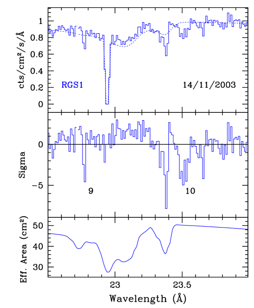
Figure 1: The ToO (left) and the archival (right) RGS–1 spectra of Mkn 421 in the [22.5–24] Å  band, together with the best–fit power–law models (upper panels). In the right panel, the solid and the dotted lines refer to the first and the second exposures of November 4, 2002, respectively, the short–dashed one represents the December 1^st, 2002 data while the long–dashed data are those taken in June 2003. In the middle panel we report the residuals left by the best–fit models and in the bottom panel the RGS–1 effective areas.

Residuals at $\sim 23.5$ Å  can be observed in the middle panels of Fig. 1, which are very likely produced by the interstellar neutral oxygen. Firstly, we fitted the ToO observation with a power–law + one Gaussian, then we simultaneously fitted the four archival spectra. Finally we fitted the five spectra together. The best–fit line position during the ToO observation is $23.510\pm 0.007$ Å, which is consistent with the archival data result ($23.507\pm 0.013$ Å). Fitting simultaneously all the spectra we obtained $\lambda=23.510\pm 0.007$ Å.
This value is slightly higher than the theoretical position found by Mc Laughlin & Kirby (1998; $\lambda=23.467$ Å), but it is consistent with the results of many authors, obtained through different experimental techniques (see Table 2).

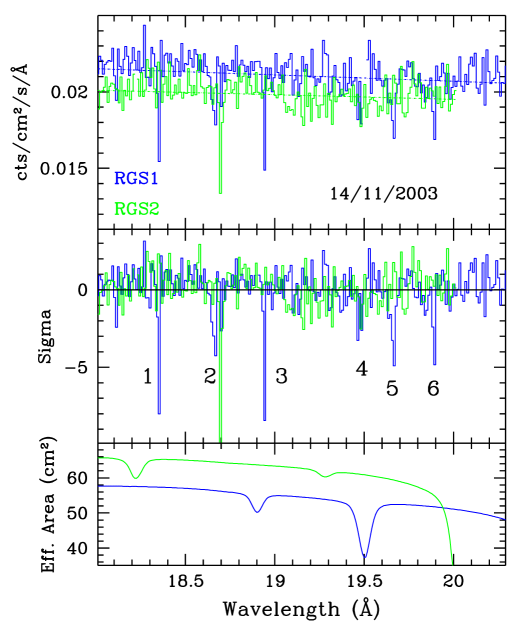
Figure 2: The RGS–1 (dark gray data) and the RGS–2 [18–20.3] Å  spectra (light gray data) of Mkn 421 during the ToO observation of November 2003. We also show the respective best–fit power–law models (dashed lines). In the mid panel we report the residuals left by the best–fit models and in the bottom panel the effective areas. The RGS–2 effective area decays above $\sim 20$ Å  because of the CCD–4 failure.

$\lambda$ (Å)	Method	Ref.
23.467	Theoretical	1
$23.489\pm 0.004$	Experimental	2
$23.536\pm 0.002$	Experimental	3
$23.52\pm 0.03$	Chandra, X0614+091	4
$23.509^{+0.008}_{-0.018}$	Chandra, PKS 2155-304	5
$23.50\pm 0.01$	XMM	6
$23.510\pm 0.015$	XMM, PKS 2155-304	7
$23.510\pm 0.007$	XMM, Mkn 421	ToO obs.
$23.507\pm 0.013$	XMM, Mkn 421	Arch. data
$23.510\pm 0.013$	XMM, Mkn 421	Total

Table 2: Neutral oxygen wavelengths (1s–2p transition). 1) Mc Laughlin & Kirby, 1998; 2) Krause 1994; 3) Stolte et al. 1997; 4) Paerels et al. 2001; 5) Nicastro et al. 2002; 6) de Vries et al. 2003; 7) Cagnoni et al. 2004.

In particular, it is in good agreement ($<1\,\sigma$) with other XMM–Newton and Chandra observations. Therefore, we shall not apply wavelength corrections to our data.

3.1 The [18–20.3] Å  spectra

In this energy range we can directly compare the RGS–1 and RGS–2 data. In Fig. 2 we show the RGS–1 (dark gray lines) and the RGS–2 spectra (light gray lines) of the ToO observation, together with the best–fit absorbed power–law model (dotted lines). We report also the residuals (in terms of sigmas, mid panels) and the effective area of the instruments (bottom panels) during the exposure. In Fig. 3, we show the same plots for the archival observations. We display as solid and dotted lines the first and the second exposures of November 4, 2002, respectively, as a short–dashed line the December 1^st, 2002 data and as a long–dashed line the June 1^st data.

Figure 3: The RGS–1 [18–20.3] Å  (left) and the RGS–2 [18–20] Å  (right) archival spectra of Mkn 421, together with the best–fit power–law models (upper panels). The solid and dotted data refer to the first and the second exposures of November 4, 2002, respectively, the short–dashed ones represent the December 1^st, 2002 data while the long–dashed ones the June 2003 data. In the mid panel we report the residuals left by the best–fit models and in the bottom panel the effective areas. We limit the RGS–2 plot to the [18–20] Å  range because of the CCD–4 failure.

Several features with significance $\gtrsim 3\,\sigma$ are shown in all the RGS–1 spectra. Two of them, the numbers 1 and 4, are located in some of the archival observations at the same energies as large structures in the effective area curves. Furthermore, they cannot be observed in the corresponding RGS–2 residuals, in regions where the effective areas are smooth. Their origin is very likely instrumental and we shall exclude them from further analysis.
We then fitted the RGS–1 spectra again, with an absorbed power–law model plus four Gaussian profiles to reproduce the residuals 2, 3, 5 and 6. In Table 3 we report the best–fit parameters of each Gaussian.

RGS–1 [18–20] Å
Feature	$\lambda$	FWHM	k
number	(Å)	(mÅ)	( cts cm-2 s-1 Å-1)
ToO observation
2	$18.661\pm 0.004$	$24^{+9}_{-6}$	$-0.0040\pm 0.0011$
3	$18.937\pm 0.001$	$8\pm 1$	$0.0111\pm 0.0023$
5	$19.662\pm 0.005$	$30\pm 10$	$-0.0040\pm 0.0010$
6	$19.890\pm 0.001$	$8.5^{+1.5}_{-1}$	$-0.0098\pm 0.0031$
Archival data
2	$18.683\pm 0.001$	$15.2^{+3}_{-2}$	$-0.319\pm 0.048$
3	$18.9585\pm 0.001$	$14.5\pm 2$	$-0.349\pm 0.051$
5	$19.681\pm 0.002$	$15\pm 3$	$-0.266\pm 0.053$
6	$19.910\pm 0.002$	$16\pm 3$	$-0.303\pm 0.050$
Total
2	$18.680\pm 0.004$	$33^{+9}_{-7}$	$-0.147\pm 0.026$
3	$18.953\pm 0.003$	$28^{+5}_{-4}$	$-0.177\pm 0.029$
5	$19.676\pm 0.003$	$23^{+5}_{-4}$	$-0.166\pm 0.032$
6	$19.904\pm 0.004$	$33^{+8}_{-7}$	$-0.128\pm 0.027$

Table 3: Best–fit parameters of the power–law plus four Gaussians model reproducing the [18–20] Å  RGS–1 spectra of Mkn 421. The error bars refer to the 90% confidence intervals.

Besides investigating the corresponding RGS–2 spectra, we also checked the reality of these features by studying a RGS–1 spectrum of the Crab taken in August 8, 2002 (Obs. Id. 0153750501). The Crab nebula, a Galactic source, has a very intense featureless power–law continuum and is therefore very useful to discriminate between the possible origins of the observed features. We reduced the Crab data as described in the previous Sections. In Fig. 4 we report the residuals (upper panel) given by the best–fit power–law model in the [18–20] Å  range and the relative effective area (lower panel).

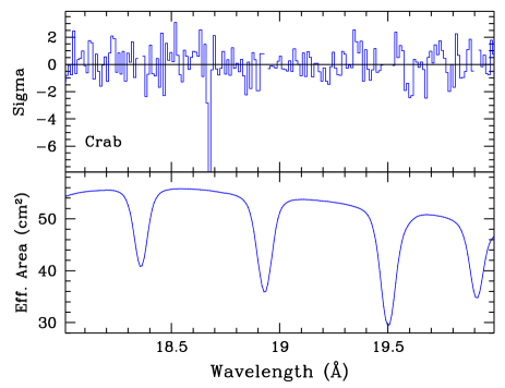
Figure 4: Residuals left by the best–fit power–law model to the [18–20] Å  RGS–1 spectrum of the Crab (upper panel). In the lower panel we show the relative RGS–1 effective area.

We summarise our results as follows:

• Feature 2 (18.680 Å): we found large residuals ($5-6\,\sigma$) close to the observer–frame wavelength of the OVII K$\beta$ transition, in a smooth region of the RGS–1 effective area. This identification, however, is still controversial. The RGS–2 data do not unambiguously confirm the RGS–1 results. During the first ToO observation and during the second one of November 4, 2002, the RGS–2 effective area was smooth and we observed a very narrow feature at a slightly higher wavelength ($18.697\pm 0.002$ Å, FWHM =$14\pm 3$ mÅ  and $\lambda=18.718\pm 0.004$ Å, FWHM = $17\pm 8$ mÅ, respectively). However, a large structure is present in the RGS–2 effective areas of the other observations. Furthermore, we also observed large residuals ($\sim 8\,\sigma$) in the RGS–1 Crab spectrum ($18.674^{+0.002}_{-0.003}$ Å). This implies a Galactic or an instrumental origin: the astronomical nature of this feature is still questionable.

• Feature 3 (18.953 Å): large residuals ($5-6\,\sigma$) are observed at the zero–redshift wavelength of the OVIII K$\alpha$ line. This identification also is quite doubtful. This line is located close to a RGS–1 effective area feature (at $\sim 18.9$ Å) and cannot be observed in the RGS–2 spectra, where the effective areas are smooth. If the RGS–2 response is well calibrated, this feature must be instrumental and the RGS–1 residuals are probably caused by calibration uncertainties of the effective area structure at $\sim 18.9$ Å.

• Feature 5 (19.676 Å): this $\sim 3\,\sigma$ feature is observed in all the RGS–1 spectra, but it is not present in the corresponding RGS–2 data. Also the RGS–1 Crab spectrum displays small residuals ($\sim 2\,\sigma$) at $19.673$ Å. The absence of this line in the RGS–2 suggests a very likely instrumental origin.

• Feature 6 (19.904 Å): the RGS–1 residuals ($\sim 4\,\sigma$) are not observed in the RGS–2 spectra. In this case, the comparison with the Crab spectrum is useless, since the corresponding effective area is characterized by a large feature. This line is probably instrumental.

3.2 The [21–22] Å  spectra

Since the ToO and the archival spectra do not display significant features in the [20–21] Å  range, we now concentrate on the [21–22] Å  interval, where line detections have been claimed by other authors. In Fig. 5 we show the [21–22] Å  RGS–1 data of the ToO (left) and of the archival observations (right).

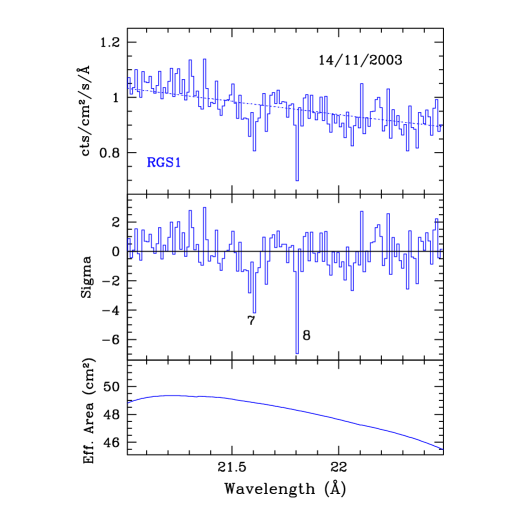
Figure 5: The RGS–1 spectra of Mkn 421 in the [21–22] Å  range. In the left panel we show the November 2003 ToO spectrum and in the right panel the archival data (upper panels), together with the best–fit models. On the right, we show with a solid and a dotted line the two exposures of November 4, 2002, with a short–dashed line the December 1^st, 2002 data and with a long–dashed line the June 2003 data. In the middle panels we display the residuals left by the best–fit models and in the lower panels the RGS–1 effective areas of the RGS–1.

Negative residuals are present at $\sim 21.6$ Å  (label 7, $\sim 2-3\,\sigma$) and at $\sim 21.8$ Å  (label 8, $\gtrsim 2\,\sigma$) both in the ToO and in the archival spectra. We reproduced the spectra with a power–law model plus 2 Gaussians. As before, we fitted the ToO spectrum alone, then the four archival spectra simultaneously. Finally, we fitted all the spectra together. In Table 4 we give the two Gaussian best–fit parameters.

RGS–1 [21–22.2] Å
Feature	$\lambda$	FWHM	k
number	(Å)	(mÅ)	(cts cm-2 s-1 Å-1)
ToO spectrum
7	$21.5915\pm 0.013$	$78^{+28}_{-25}$	$-0.0025\pm 0.0007$
8	$21.801\pm 0.0005$	$7\pm 1$	$-0.018\pm 0.005$
Archival data
7	$21.612\pm 0.010$	$68^{+19}_{-16}$	$-0.012\pm 0.002$
8	$21.819\pm 0.001$	$12\pm 2$	$-0.342\pm 0.068$
Total
7	$21.603\pm 0.008$	$81^{+17}_{-15}$	$-0.109\pm 0.019$
8	$21.823\pm 0.001$	$6\pm 2$	$-0.277\pm 0.059$

Table 4: Best–fit parameters of the power–law plus two Gaussians model reproducing the [21–22] Å  Mkn 421 spectra taken by the RGS–1. The errorbars refer to the 90% confidence intervals.

Because of readout failures in the RGS–2 CCD–4 we cannot compare the RGS–1 and the RGS–2 data. To check the reality of the two RGS–1 features, we investigated the spectrum of the Crab nebula. In Fig. 6 we show the residuals left by a power–law model in the RGS–1 Crab spectrum (upper panel) and the effective area of the instrument (lower panel).

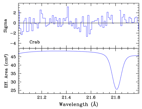
Figure 6: Residuals left by the best–fit power–law model to the [21–22] Å  RGS–1 spectrum of the Crab (upper panel). In the lower panel we show the relative RGS–1 effective area.

We summarize the results for this energy range as follows:

• Feature 7 (21.603 Å): broad residuals can be observed in each Mkn 421 spectrum at the observer–frame wavelength of the OVII K$\alpha$ transition. The line is not present in the Crab spectrum. We believe it is caused by an astronomical OVII K$\alpha$ absorbing system.

• Feature 8 (21.823 Å): large residuals can be observed at this wavelength (up to $\sim 4\,\sigma$, December 1^st). Unfortunately, the comparison with the Crab data is useless because of a large effective area structure. In previous papers, this line was usually interpreted as an OVII K$\alpha$ absorbing system at redshift $z\sim 0.01$. With the present data, however, we cannot draw firm conclusions about its astronomical origin.

3.3 The [22.5–24.5] Å  spectra

In Fig. 1 we showed the [22.5–24.5] Å  RGS–1 spectra of the ToO (left) and of the archival observations (right).
This energy range is characterized by the presence of broad instrumental features caused by oxygen absorption as well as by the interstellar absorption around the oxygen K edge (see e.g. de Vries 2003). Combining several Mkn 421 and PKS 2155-304 RGS–1 spectra and comparing them with strongly absorbed Galactic sources, de Vries et al. (2003) showed the presence of instrumental features around 23.05 Å  and 23.35  Å. The updated calibration files we used to analyze our Mkn 421 data account for these structures (see the large features in the RGS–1 effective areas of Fig. 1), even if large residuals are still present at $\sim 23.35$ Å, probably caused by uncertainties in calibrating the instrumental molecular oxygen absorption (de Vries 2003).
We observed two features at a wavelength where the effective areas are smooth, one of which (label 10 of Fig.1) is the already–discussed interstellar neutral oxygen 1s–2p absorption line at $\sim 23.5$ Å  (see Section 4.0.1). We fitted the [22.5–24.5]  Å  spectra with a power–law + 2 Gaussians models to reproduce the residuals and we report the results in Table 5.

RGS–1 [22.5–24.5] Å
Feature	$\lambda$	FWHM	k
number	(Å)	(mÅ)	(cts cm-2 s-1 Å-1)
ToO observation
9	$22.770\pm 0.001$	$9\pm 1$	$-0.011\pm 0.003$
10	$23.510\pm 0.007$	$64^{+13}_{-12}$	$-0.004\pm 0.001$
Archival data
9	$22.789^{+0.003}_{-0.002}$	$15.5\pm 5$	$-0.225\pm 0.0665$
10	$23.510\pm 0.013$	$64^{+26}_{-20}$	$-0.082\pm 0.029$
Total
9	$22.778\pm 0.001$	$6^{+2}_{-1}$	$-0.304\pm 0.086$
10	$23.510\pm 0.007$	$71^{+13}_{-11}$	$-0.133\pm 0.020$

Table 5: Best–fit parameters of the power–law plus three Gaussians model reproducing the [22–24] Å  Mkn 421 spectra taken by the RGS–1. The error bars refer to the 90% confidence intervals.

As a comparison, we show in Fig. 7 the residuals left by a power–law model of the Crab spectrum. In this case, the extremely large count rate strongly suggests calibration uncertainties and we therefore avoide reproducing the [22.9–23.6] Å  residuals.

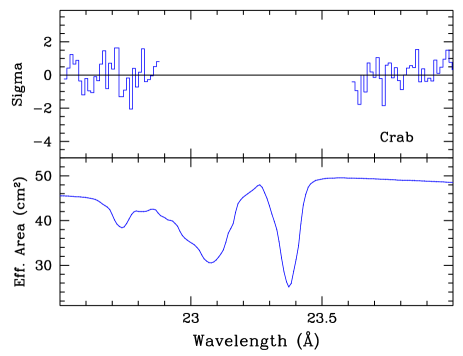
Figure 7: Residuals left by the best–fit power–law model to the [22.5–24] Å  RGS–1 spectrum of the Crab (upper panel). In the lower panel we show the corresponding RGS–1 effective area. We did not display the residuals in the [22.9–23.6] Å  range which is affected by large instrumental features.

We summarize the results as follows:

• Feature 9 (22.778 Å): each Mkn 421 spectrum display residuals ($2-3\,\sigma$) near a small structure of the RGS–1 effective areas (at $\sim 22.75$ Å). This feature cannot be observed in the Crab spectrum. In a previous paper, de Vries et al. (2003) tentatively identified this line as an OIV blend produced in the local intergalactic medium.

• Feature 10 (23.510 Å): this line was observed in all the RGS–1 spectra and can be identified with the interstellar neutral oxygen (1s–2p) absorption line (see the wavelength calibration Section).

Feature	RGS–1	RGS–2	Crab	Literature	Other
number	$\lambda$ (Å)				sources
2	$18.680\pm 0.004$	$18.697$ (ToO)	$18.674^{+0.002}_{-0.003}$	YES (C01–XMM)	PKS 2155-304 (N02–Cha)
		$18.718$ (4/11/02)		NO (N01–Cha)	PKS 2155-304 (C04–XMM)
		instrumental		YES (N03–Cha)
3	$18.953\pm 0.003$	NO	instrumental	YES (C01–XMM)	PKS 2155-304 (N02–Cha)
				NO (N01–Cha)	3C 273 (F03–Cha)
				YES (N03–Cha)	NO PKS 2155-304 (C04–XMM)
5	$19.676\pm 0.003$	NO	NO	NO	NO
6	$19.904\pm 0.004$	instrumental	instrumental	NO	PKS 2155-304 (C04–XMM)
					NO PKS 2155-304 (N02–Cha)
7	$21.603\pm 0.008$	no data	NO	YES (C01–XMM)	PKS 2155-304 (N02–Cha)
				NO (N01–Cha)	PKS 2155-304 (C04–XMM)
				YES (N03–Cha)	3C 273 (F03–Cha)
8	$21.823\pm 0.001$	no data	instrumental	YES (C01–XMM)	PKS 2155-304a (XMM)
				YESb (N01–Cha)	NO PKS 2155-304 (C04–XMM)
				YES (N03–Cha)
9	$22.778\pm 0.001$	no data	NO	YES (dV03–XMM)	PKS 2155-304 (dV03–XMM)
			near		PKS 2155-304 (dV03–Cha)
			instrumental		PKS 2155-304 (C04–XMM)
			feature		NO ScoX1(dV03–XMM)
					NO 4U 0614+91 (dV03–XMM)
10	$23.510\pm 0.007$	no data		YES (dV03–XMM)	PKS 2155-304 (P01–Cha)
					PKS 2155-304 (N02–Cha)
					PKS 2155-304 (C04–XMM)

Table 6: Summary of absorption features observed in the RGS spectrum of Mkn421. ^a: archival data analyzed by us. ^b: detected in one of the two observations. C01: Cagnoni (2001); N01: Nicastro et al. (2001); P01: Paerels et al. (2001); N02: Nicastro et al. (2002); N03: Nicastro et al. (2003); dV03: de Vries (2003); F03: Fang et al. (2003); C04: Cagnoni et al. (2004).

4 Discussion

In the previous Sections we showed the presence of several absorption features in the X–ray spectra of Mkn 421 taken with the RGS–1 aboard XMM–Newton. The X–ray spectra are similar, displaying the same absorption lines during all 5 observations over one year. We discarded some of the lines because they are very likely instrumental. Among the rest, we found the well–known interstellar neutral oxygen 1s–2p line at $\sim 23.5$ Å  (see e.g. de Vries et al. 2003). We observed features at the observer–frame wavelengths of the expected WHIM lines, i.e. at $\sim 18.6$ Å  (OVII K$\beta$), at $\sim 18.95$  Å  (OVIII K$\alpha$) and at $\sim 21.6$ Å  (OVII K$\alpha$), which were also reported in some previous works (e.g. Cagnoni 2001; Nicastro 2003). We cannot confirm the detection of the local NeIX absorption feature at $\sim 13.4$ Å  (Cagnoni 2001; Rasmussen et al. 2003). We also found two small features, at $\sim 21.8$ Å  and at $\sim 22.78$ Å, which were identified in previous papers as a $z\sim 0.01$ OVII K$\alpha$ line (Cagnoni 2001; Nicastro 2003) and as a local OIV blend (de Vries et al. 2003), respectively.
However, the astronomical origin of some of these lines is doubtful. The comparison of the RGS–1 data with the corresponding RGS–2 spectra (where available), with a RGS–1 spectrum of the Crab nebula and with the literature data suggests that some of these lines are probably instrumental. The absence of an RGS–1 feature in the corresponding RGS–2 spectrum strongly points towards an instrumental origin of the line. Also the literature data are not conclusive: none of the reported lines were always detected during the XMM–Newton and the Chandra observations. We resume these comparisons in Table 6.
The suspicions about the astronomical nature of some of the lines are furtherly strengthened by their extreme narrowness (see Table 7). The features at $18.95$ Å, $\sim 21.8$ Å  and at $\sim 22.78$ Å  are much smaller (by a factor $\gtrsim 4$) than the RGS–1 spectral resolution ($\lambda/\Delta\lambda_{\rm FWHM}<500$; see XMM–Newton users’ handbook). The feature at $\sim 18.6$ Å  is marginally consistent with the instrumental performances only during the ToO observation. Even in this case, however, both the corresponding RGS–2 line and the feature in the Crab spectrum are narrower than the RGS response ($\lambda/\Delta\lambda_{\rm FWHM}>1000$), supporting an instrumental nature. We therefore conclude that while the features at $\sim 21.6$ Å, at $\sim 23.5$ Å  can be identified as astronomical lines, all the others are probably of instrumental origin (although some of them have been reported as real astronomical lines in previous works by other authors).

Feature	$\lambda$	$\lambda/\Delta\lambda_{\rm FWHM}$
number	(Å)	ToO	Archival	Total
2	18.680	$780^{+190}_{-290}$	$1230^{+160}_{-240}$	$570^{+120}_{-150}$
3	18.953	$2370\pm 300$	$1310\pm 180$	$680^{+100}_{-120}$
7	21.603	$280^{+90}_{-100}$	$320^{+70}_{-90}$	$270\pm 50$
8	21.823	$3110\pm 440$	$1820\pm 300$	$3640\pm 1200$
9	22.778	$2530\pm 280$	$1470\pm 470$	$3800^{+630}_{-1260}$
10	23.510	$370\pm 70$	$370^{+110}_{-150}$	$330^{+50}_{-60}$

Table 7: $\lambda/\Delta\lambda_{\rm FWHM}$ ratios for the possible astronomical features observed in the RGS–1 spectra of Mkn 421. The instrumental resolving power is $\lambda/\Delta\lambda_{\rm FWHM}<500$.

The feature located at $23.510\pm 0.007$ Å  is the well–known interstellar neutral oxygen (1s–2p) absorption line which we discussed in a previous Section. The feature at $21.603\pm 0.008$ Å  is very close to the OVII K$\alpha$ transition ($\lambda=21.602$ Å  in the observer frame), the strongest WHIM signature predicted by the simulations (e.g. Hellsten, Gnedin & Miralda–Escudé 1998). An OVII absorbing system was already observed at zero redshift toward Mkn 421 (Cagnoni 2001; Nicastro 2003) as well as toward other sources as PKS 2155-489 (Nicastro et al. 2002; Cagnoni et al. 2004), 3C 273 (Fang et al. 2002) and H 1821+643 (Mathur et al. 2003), while Mckernan et al. (2004) studied the sightlines toward 15 AGNs, finding evidence of local hot gas in various cases. This has been attributed either to the WHIM within the local group of galaxies (e.g. Nicastro et al. 2002, McKernan et al. 2004) or to radiatively cooling gas inside our Galaxy (e.g. Heckmann et al., 2002; McKernan et al. 2004).
The average equivalent width of the $21.603$ Å  line is EW=$9.6^{+3.9}_{-3.1}$ mÅ, consistent with that found by Cagnoni (2001) in her composite spectrum (EW=$12.67^{+1.59}_{-1.54}$ mÅ). Since the equivalent width of our OVII K$\alpha$ line falls in the linear branch of the curve of growth calculated by Nicastro et al. (2002), it should be produced in an unsaturated absorption regime. Using Fig. 4 of Nicastro et al. (2002), we can therefore calculate the column density of OVII toward Mkn 421, N${}_{\rm OVII}\sim 4\times 10^{15}$ cm^-2. A similar result is also obtained using the curves of growth calculated by Mathur et al. (2003): the OVII column density is in the range $[4-10]\times 10^{15}$ cm^-2, depending on the assumed velocity parameter of the gas.
Assuming an upper limit to the equivalent width of the non–detected OVIII K$\alpha$, we could set an upper limit to the temperature of the absorbing gas. If a line is not saturated, as in our case, the equivalent width produced by an ion $X^{i}$ can be written as EW$(X^{i})\propto A(X)n_{X^{i}}$ (Nicastro et al. 1999b), where $A(X)$ is the relative abundance of the element $X$ compared to H and $n_{X^{i}}$ is the relative density of the ion $i$ of the element $X$. We assumed therefore that the OVIII K$\alpha$ at $\sim 18.97$ Å  was characterized by the same FWHM of the observed OVII K$\alpha$ (FWHM = $0.081^{+0.017}_{-0.015}$ Å) and by an amplitude of three times the uncertainty on the continuum at the line wavelength. We obtained an average EW=$1.3\pm 0.3$ Å. Using the OVIII/OVII ratio vs temperature $T$ plot calculated by Nicastro et al. (2002), we obtained an upper limit for the gas temperature $T\lesssim 1.6\times 10^{6}$ K in the case of a Galactic density ($n_{e}=1$ cm^-3). In the case of the extreme extragalactic low-denisity solution, $n_{e}=10^{-6}$ cm^-3, the gas temperature would be much lower than $10^{5}$ K, while for higher density values, up to $n_{e}=5\times 10^{-5}$ cm^-3 (Nicastro et al. 2005a), the gas temperature would be compatible with values of the order of few times $10^{5}$ K. Heckman et al. (2002) suggested that the zero redshift X–ray absorption lines observed toward PKS 2155-304 by Nicastro et al. (2002) originated in a radiatively cooling gas inside our Galaxy. This would be the case also for Mkn 421 if we assume a low extragalactic density. The gas would then be too cool to be identified as the searched-for WHIM, whose temperature is predicted to be greter than $10^{5}$ K (e.g Hellsten, Gnedin & Miralda–Escudé 1998). However, if we assume a larger density value, then our data are still compatible with a WHIM with a temperature of the order of a few times $10^{5}$ K.

5 Conclusions

We presented the analysis of the data of the high resolution RGS spectrometers aboard XMM–Newton during a ToO observation of Mkn 421 performed in November 2003. The pointing was triggered since the source was in a high state of activity in the X–ray band. We compared these data with 3 archival RGS observations of the same source performed in November and December 2002 and with one performed in June 2003. We summarize the main results:

• The integrated [7–36]  Å  RGS–1 and RGS–2 spectra are well fitted by a broken power–law model, with a hard spectral index ($\alpha_{1}\sim 0.6-0.9$) below 0.7–0.8 keV softening toward higher energies ($\alpha_{2}\sim 1.0-1.3$). The RGS–2 spectra show systematically softer slopes and lower fluxes.

• We compared the RGS spectra to the corresponding EPIC–PN spectra in the common well–calibrated energy range: [0.6–1.77] keV. The EPIC–PN spectra are significantly softer, always showing spectral indices $\alpha>1$, with fluxes larger by 5–10%.

• We focused on small sections, 2–3 Å  wide, of the RGS–1 spectra, looking for absorption features. We found several lines which are common to all the observed spectra. However, we found evidence that several of them are instrumental: their proximity to effective area features, their absence in the corresponding RGS–2 spectra or their extreme narrowness (much smaller than the instrumental resolution). We found that only two features are very likely of astronomical origin: one at $\sim 23.5$ Å  and one at $\sim 21.6$ Å.

• We identified the feature at $23.5$ Å  as interstellar neutral oxygen absorption, as proposed e.g. by de Vries et al. (2003). We found a best–fit wavelength of $23.510\pm 0.007$ Å, slightly larger than the theoretical position proposed by Mc Laughlin & Kirby (1998), but fully consistent with the experimental results of several authors.

• The feature at $\sim 21.6$ Å  corresponds to a zero–redshift OVII K$\alpha$ transition. Assuming a 3$\sigma$ upper limit on the non–detected corresponding OVIII K$\alpha$, we calculated an upper limit for the gas temperature. We found that an extragalactic gas with a very low density would be much colder than the predicted WHIM temperature range. In this case this line would have a Galactic origin, produced by a radiatively cooling gas, as proposed by Heckman et al. (2002). For an extragalactic gas with higher density, WHIM with a temperature of a few times $10^{5}$ K would still be compatible with the data.

We conclude from our analysis that, with the current knowledge of the XMM-Newton grating performances and the sensitivity provided by our spectra, we could not find firm evidence of the Warm/Hot Intergalactic Medium toward Mkn 421.

Note added in proof After this paper was accepted, the Nicastro et al. (2005b) paper appeared in the literature. Nicastro et al. were able to observe Mkn 421 in much higher states with the grating on board the Chandra satellite. Thanks to the higher signal to noise ratio they were able to identify many more astronomical lines that allow them to derive for the first time a population of baryons in two intervening WHIM systems at $z=0.011$ and $z=0.027$ and to study in detail the zero–redshift system (Williams et al. ApJ submitted).

Appendix A RGS spectral analysis and comparison with EPIC-PN

First, we analyzed the RGS–1 and RGS–2 spectra in the full [0.34–1.77] keV energy range ([7–36] Å), where the calibration uncertainties are smaller than 10%. We rebinned the RGS data to have at least 2000 counts per bin and added a systematic error of $3\%$. We fitted the data with an absorbed power–law and a broken power–law model, fixing the absorption parameter to the Galactic value (N${}_{\rm H}=1.61\pm 0.1\times 10^{20}$ cm^-2; Lockman & Savage 1995). In Table 8 we report the best–fit parameters of each observation. The RGS–2 spectra display systematically steeper slopes and lower fluxes than the RGS–1, as reported in the calibration paper on the radio–loud narrow–line Seyfert 1 galaxy PKS 0558-508 (Kirsch 2003).

   

Figure 8: The RGS–1 spectrum of the ToO observation of November 14, 2003. An absorbed power–law model is not able to reproduce the data well (left panel), while a broken power–law model fits the data better (right panel). We fixed the absorption parameter to the Galactic value. The spectra were rebinned in order to have at least 2000 counts per bin. The other RGS spectra display similar behaviors.

Inst.	$\alpha_{1}$	Eb	$\alpha_{2}$	F1keV	F0.5-1.5keV	$\chi^{2}_{r}/d.o.f.$
		(keV)		($\nu$Jy)	($\times 10^{-10}$)a
Exp. 0136540301
RGS–1	$0.99$			101.9	2.71	3.26/127
RGS–1	$0.755^{+0.055}_{-0.035}$	$0.74^{+0.1}_{-0.03}$	$1.27^{+0.11}_{-0.04}$	104.9	2.72	0.91/125
RGS–2	$1.05$			92.4	2.48	4.24/125
RGS–2	$0.81\pm 0.03$	$0.80^{+0.02}_{-0.03}$	$1.46^{+0.04}_{-0.06}$	97.3	2.51	0.90/125
Exp. 0136540401
RGS–1	$0.93$			120.1	3.16	3.89/137
RGS–1	$0.63^{+0.03}_{-0.06}$	$0.69^{+0.02}_{-0.04}$	$1.20^{+0.03}_{-0.04}$	123.2	3.19	0.94/135
RGS–2	$0.94$			115.9	3.05	2.52/144
RGS–2	$0.77^{+0.04}_{-0.02}$	$0.79^{+0.03}_{-0.05}$	$1.18\pm 0.04$	121.0	3.07	1.21/142
Exp. 0136541001
RGS–1	$0.90$			72.8	1.91	2.83/227
RGS–1	$0.64\pm 0.02$	$0.67^{+0.03}_{-0.02}$	$1.11\pm 0.02$	75.0	1.92	0.92/225
RGS–2	$0.92$			68.7	1.81	2.5/240
RGS–2	$0.74^{+0.03}_{-0.02}$	$0.76^{+0.03}_{-0.04}$	$1.17^{+0.02}_{-0.04}$	71.6	1.82	0.97/238
Exp. 0158970101
RGS–1	1.06			74.0	1.98	3.5/138
RGS–1	$0.80\pm 0.04$	$0.71^{+0.02}_{-0.04}$	$1.33^{+0.03}_{-0.04}$	75.3	2.00	1.16/136
RGS–2	1.10			68.5	1.85	2.3/139
RGS–2	$0.92^{+0.03}_{-0.04}$	$0.76\pm 0.05$	$1.35\pm 0.04$	71.2	1.86	0.83/137
Exp. 0150498701
RGS–1	$0.80$			186.5	4.83	3.17/454
RGS–1	$0.56\pm 0.02$	$0.71\pm 0.02$	$1.015\pm 0.015$	192.4	4.87	1.13/452
RGS–2	0.82			174.3	4.52	2.42/490
RGS–2	$0.64\pm 0.02$	$0.73\pm 0.02$	$1.02^{+0.01}_{-0.02}$	179.8	4.56	1.08/488
Parabolic model
	a		b
Exp. 0136540301
RGS–1	$1.21^{+0.02}_{-0.03}$		$0.77\pm 0.08$	110.9	2.74	1.02/126
RGS–2	$1.33^{+0.02}_{-0.03}$		$0.96^{+0.06}_{-0.1}$	101.2	2.52	1.1/126
Exp. 0136540401
RGS–1	$1.17^{+0.02}_{-0.03}$		$0.86^{+0.05}_{-0.09}$	131.5	3.21	1.11/136
RGS–2	$1.10^{+0.02}_{-0.03}$		$0.58^{+0.05}_{-0.09}$	125.4	3.08	1.36/143
Exp. 0136541001
RGS–1	$1.09^{+0.01}_{-0.04}$		$0.67^{+0.04}_{-0.07}$	79.3	1.93	1.07/226
RGS–2	$1.10^{+0.01}_{-0.02}$		$0.60^{+0.05}_{-0.06}$	74.5	1.83	1.13/239
Exp. 0158970101
RGS–1	$1.28^{+0.02}_{-0.03}$		$0.77^{+0.06}_{-0.08}$	80.6	2.01	1.33/137
RGS–2	$1.29\pm 0.02$		$0.65^{+0.06}_{-0.09}$	74.3	1.87	0.91/138
Exp. 0150498701
RGS–1	$0.96\pm 0.01$		$0.65^{+0.05}_{-0.03}$	204.0	4.91	1.25/453
RGS–2	$0.97^{+0.01}_{-0.02}$		$0.53^{+0.03}_{-0.04}$	188.6	4.57	1.25/489

Table 8: Best–fit parameters of the RGS spectra reproduced with power–law, broken power–law and parabolic models. We fixed the absorption parameter to the Galactic value. The error bars refer to the 90% confidence interval. ^a: erg cm^-2 s^-1.

Figure 9: EPIC–PN (filled circles), RGS–1 (empty circles) and RGS–2 (crosses) spectra of Mkn 421 during the ToO observation of November 14, 2003, fitted together with a broken power–law model (with Galactic absorption value). For plotting purposes, we rebin the the RGS data to have at least 15000 counts in each bin. The RGS spectra are significantly harder than the EPIC–PN spectrum. For clarity, we omitted the residual error bars.

The power–law model cannot reproduce the spectra: the $\chi^{2}_{r}$ are always larger than 2 (e.g. Fig. 8). The broken power–law model significantly improves the quality of the fit: the spectra of Mkn 421 are hard up to $\sim 0.7-0.8$ keV and soften toward higher energies. We also tried to reproduce the steepening with the logarithmic parabolic model proposed by Massaro et al. (2003a,b), which we already applied to the corresponding EPIC–PN spectra (Ravasio et al. 2004), as well as to the BeppoSAX spectra of other similar sources, such as 1ES 1959+650 (Tagliaferri et al. 2003). This curved model reproduces the data well, even if, in all cases, the broken power–law gives better results.

To check the quality and the good calibration of these data, we compared them to the corresponding EPIC–PN spectra in the common well–calibrated energy range ([0.6–1.77] keV). The RGS and the EPIC–PN data are well fitted by a broken power–law model softening toward higher energies. The EPIC–PN spectra are significantly softer, always with slopes $\alpha>1$, while the RGS spectra are hard up to $\sim 0.8$ keV. The greater softness of the EPIC–PN was shown also by Kirsch (2003), using an XMM–Newton observation of PKS 0558-508. This is very clear in Fig. 9, where we plot the RGS and the EPIC–PN spectra of the ToO observation. Furthermore, the EPIC–PN fluxes are larger by $\sim 5-10\%$. As an example, we report in Table 9 the best–fit parameters of the power–law and broken power–law models for the November 2003 ToO observation. These calibration differences, however, are not important for our search for WHIM features. We focused on such small sections of the RGS spectra (2–3 Å  wide) that the continuum uncertainties can be neglected.

Inst.	$\alpha_{1}$	Eb	$\alpha_{2}$	F1keV	F0.6-1.5keV	$\chi^{2}_{r}/d.o.f.$
		(keV)		($\mu$Jy)	($\times 10^{-10}$)a
November 14, 2003
RGS–1	$0.97\pm 0.01$			188.3	4.17	1.13/246
RGS–1	$0.76\pm 0.07$	$0.80^{+0.05}_{-0.03}$	$1.03^{+0.03}_{-0.02}$	192.3	4.18	0.91/244
RGS–2	$0.97\pm 0.01$			176.4	3.91	1.11/330
RGS–2	$0.75^{+0.09}_{-0.12}$	$0.78\pm 0.04$	$1.02\pm 0.02$	180.0	3.90	1.0/328
PN	$1.34\pm 0.01$			202.3	4.35	6.6/45
PN	$1.23^{+0.02}_{-0.03}$	$1.02\pm 0.06$	$1.43\pm 0.02$	207.2	4.35	0.81/43

Table 9: Best–fit parameters of the ToO RGS and EPIC–PN spectra fitted with power–law and broken power–law models, in the common energy range ([0.6–1.77] keV). The absorption parameter was fixed to the Galactic value. Systematic errors of 3% and of 0.5 % were added to the RGS and to the EPIC–PN data, respectively. The error bars refer to the 90% confidence interval for one parameter. ^a: erg cm^-2 s^-1.

References

- Aldcroft et al., (1994) Aldcroft, T., Elvis, M., McDowell, J. & Fiore, F. 1994, ApJ, 437, 584
- Burles & Tytler, (1998) Burles, S. & Tytler, D. 1998, ApJ, 499, 699
- Cagnoni (2001) Cagnoni, I. 2001, astro–ph/0212070
- Cagnoni et al., (2004) Cagnoni, I., Nicastro, F., Maraschi, L., Treves, A., Tavecchio, F., 2004, ApJ, 603, 449
- Cen & Ostriker, (1999) Cen, R. & Ostriker, J.P. 1999, ApJ, 514, 1
- Cen et al., (2001) Cen, R. , Tripp, T.M., Ostriker, J.P. & Jenkins, E.B. 2001, ApJ, 559L, 5
- Davé et al., (2001) Davé, R., Cen, R., Ostriker, J.P. et al. 2001, ApJ, 552, 473
- de Vries et al., (2003) de Vries, C.P., den Herder, J.W., Kaastra, J.S. et al. 2003, A&A, 404, 959
- Fang & Canizares, (2000) Fang, T. & Canizares, C.R. 2000, ApJ, 539, 532
- Fang et al., (2002) Fang, T., Marshall, H.L., Lee, J.C., Davis, D.S. & Canizares, C.R. 2002, ApJ, 572, L127
- Fang, Sembach & Canizares, (2003) Fang, T., Sembach, K.R. & Canizares, C.R. 2003, ApJ, 586L, 49
- Fukugita. Hogan & Peebles, (1998) Fukugita, M., Hogan, C.J. & Peebles, P.J.E. 1998, ApJ, 503, 518
- Heckman et al. (2002) Heckman, T.M., Norman, C.A., Strickland, D.K. & Sembach, K.R. 2002, ApJ, 577, 691
- Hellsten, Gnedin & Miralda–Escudé, (1998) Hellsten, U., Gnedin, N.Y. & Miralda–Escudé, J. 1998, ApJ, 509, 56
- Kirsch (2003) Kirsch, M., 2003, in XMM–EPIC status of calibration and data analysis, issue: 2.1
- Krause, (1994) Krause M.O. 1994, Nucl. Instrum. Methods B, 87,178
- Lockman & Savage, (1995) Lockman, F.J. & Savage, B.D. 1995, ApJS, 97, 1
- Ma et al., (1998) Ma, C., Arias, E.F., Eubanks, T.M. et al. 1998, AJ, 116, 516
- (19) Massaro, E., Giommi, P., Tagliaferri, G. et al. 2003a, A&A, 399,33
- (20) Massaro, E., Perri, M., Giommi, P. & Nesci, R. 2003b, subm. to A&A
- Mathur et al., (2002) Mathur, S., Weimberg, D.H. & Chen, X. 2002, in Proc. of the conference “IGM/Galaxy Connection – The Distribution of Baryons at z=0”, astro–ph/0210575
- Mathur et al. (2003) Mathur, S., Weimberg, D.H. & Chen, X. 2003, ApJ, 582, 82
- Mckernan et al. (2004) Mckernan, B., Yaqoob, T., Reynolds, C.S., 2004, ApJ 617, 232
- McLaughlin & Kirby, (1998) McLaughlin, B.M. & Kirby, K.P. 1998, J. Phys. B: At. Mol. Opt. Phys., 31, 4991
- Mulchaey et al., (1996) Mulchaey, J.S., Mushotzky, R.F., Burstein, D. & Davis, D.S. 1996, ApJ, 456, L5
- Nicastro et al., (2005) Nicastro, F., Elvis, M., Fiore, F., Mathur, S., 2005a, Proceeding of 35th Cospar, Paris 18-25 July 2004, astro-ph/0501126
- Nicastro et al., (1999) Nicastro, F., Fiore, F., Perola, G.C. & Elvis, M. 1999, ApJ, 512, 184
- Nicastro et al., (2001) Nicastro, F., Fruscione, A., Elvis, M. et al. 2001, in X–ray Astronomy 2000, ASP Conference Proceeding, Vol. 234, Eds. R. Giacconi, S. Serio & L. Stella, San Francisco: ASP, p. 511
- (29) Nicastro, F., Mathur, S., Elvis, M., Drake, J., Fang, T., Fruscione, A., Krongold, Y., Marshall, H., Williams, R., Zezas, A., 2005b, Nature 433, 495
- Nicastro et al., (2002) Nicastro, F., Zezas, A., Drake, J. et al. 2002, ApJ, 573, 157
- Nicastro et al., (2003) Nicastro, F. 2003, IAUS, 216, 170
- Paerels et al., (2001) Paerels, F., Brinkman A.C., van der Meer, R.L.J. et al. 2001, ApJ, 546, 338
- Perna & Loeb (1998) Perna, R., Loeb, A., 1998, ApJ, 503L, 135
- Rasmussen et al. (2003) Rasmussen, A., Kahn, S.M. & Paerels, F. 2003, in “The IGM/Galaxy Connection: The Distribution of Baryons at z=0”, ASSL Conference proceedings, Vol. 281, Eds. J.L. Rosenberg & M.E. Putman, p. 109
- Rauch et al., (1997) Rauch, M., Miralda–Escudé, J., Sargent, W.L.W. et al. 1997, ApJ, 489, 7
- Ravasio et al., (2004) Ravasio, M., Tagliaferri, G., Ghisellini, G. & Tavecchio, F., 2004, A&A, 424, 841
- Sembach et al. (2000) Sembach, K.R., Savage, B.D., Shull, M.D. et al., 2000, ApJ, 538, L31
- Snowden et al., (2002) Snowden S., Still M., Harrus I., Arida M. & Perry B., 2002, An introduction to XMM–Newton data analysis, NASA/GSFC XMM–Newton GOF
- Stolte et al., (1997) Stolte W.C. et al., 1997, J.Phys. B:At. Mol. Opt. Phys., 30, 4489
- Tagliaferri et al. (2001) Tagliaferri, G., Ghisellini, G. & Ravasio M. 2001, in Proceedings of the International Workshop “Blazar Astrophysics with BeppoSAX and other Observatories”, Eds. P. Giommi, E. Massaro & G. Palumbo, p.11
- Tagliaferri et al. (2003) Tagliaferri, G., Ravasio, M., Ghisellini, G. et al. 2003, A&A, 412, 711
- Tripp et al. (2001) Tripp, T.M., Giroux, L.M., Stocke, J.T. et al., 2001, ApJ, 563, 724