Probing the largest scale structure in the universe with polarization map of galaxy clusters

Abstract

We introduce a new formalism to describe the polarization signal of galaxy clusters on the whole sky. We show that a sparsely sampled, half–sky map of the cluster polarization signal at $z\sim 1$ would allow to better characterize the very large scale density fluctuations. While the horizon length is smaller in the past, two other competing effects significantly remove the contribution of the small scale fluctuations from the quadrupole polarization pattern at $z\sim 1$. For the standard $\Lambda$CDM universe with vanishing tensor mode, the quadrupole moment of the temperature anisotropy probed by WMAP is expected to have a $\sim 32\%$ contribution from fluctuations on scales below $6.3h^{-1}$Gpc. This percentage would be reduced to $\sim 2\%$ level for the quadrupole moment of polarization pattern at $z\sim 1$. A cluster polarization map at $z\sim 1$ would shed light on the potentially anomalous features of the largest scale structure in the observable universe.

1) Introduction One of the most intriguing features of the temperature anisotropy measured by WMAP Bennett:2003bz is the extremely low value of the estimated quadrupole moment. According to the WMAP team, the probability of observing such a low value, given their best–fit cosmological model, is $\sim 0.7\%$ Spergel:2003cb . Independent analysis of the WMAP data have somewhat reduced the significance of this finding (see e.g. Tegmark:2003ve ), but have also evidenced other curious results, such as the indication of a preferred direction for the quadrupole and octopole modes deOliveira-Costa:2003pu . These discoveries have raised speculations on possible non–standard topology of the Universe deOliveira-Costa:2003pu ; Cornish:2003db or inflationary physics (see e.g. Contaldi:2003zv ), and at the same time, evidenced the importance of independent observational methods to probe the largest scale structure in the Universe.

The low-$l$ moments of the present temperature anisotropies are usually assumed to probe the largest scales, but in fact they carry information about perturbations on a fairly broad range of scales. It would be highly preferable to find an observable which probes the largest scales with less contamination from intermediate ones. In this Letter we point out that the polarization signal from high–redshift clusters could be such observable.

Light scattered off a free electron is polarized, if the electron sees a quadrupole anisotropy of its incident light. This effect gives rise to interesting observable phenomena, like, for example, the large–scale polarization signal in a reionized Universe Zalda97 ; Skordis . The same effect is responsible for the major polarization signal in Sunyaeve–Zeldovich (SZ) galaxy clusters. As first pointed out by Kamionkowski:1997na , the polarization pattern of clusters at different redshifts may shed light on the quadrupole amplitude at earlier times and at different positions (see also Baumann:2003xb in relation to the low observed quadrupole moment). The cluster polarization has also been investigated as a potential tool to determine the nature of dark energy that is sensitive to the Integrated Sachs-Wolfe effect Baumann:2003xb ; Cooray:2003hd .

In this Letter we develop a transparent formalism for the calculation of the relevant observable quantities of the cluster’s polarization signal, and show that the polarization pattern at $z\sim 1$ could be a promising probe of the largest scale structure in the universe, compared with the quadrupole temperature anisotropies observed today. This finding contrasts with the naive expectation that the polarization signal of distant clusters are generated by fluctuations whose spatial scales are well within the horizon at the present Port . We also estimate how well the dark energy equation of state can be measured by the sole cluster polarization signal.

2) Formulation In this section we review the formalism to analyze the polarization signals of galaxy clusters. Throughout this Letter, we only discuss linear scalar perturbations in a flat background universe. We first introduce a fixed spherical coordinate system $\mbox{\boldmath${C}$}_{0}$ centered on an observer at $z=0$. In the coordinate system $\mbox{\boldmath${C}$}_{0}$ we denote the angular variables with $\Omega=(\theta,\phi)$ and use redshift $z$ as a radial coordinate for our past light cone. Let us consider the linear polarization generated by the local temperature anisotropy seen by a cluster labeled by $i$ at a redshift $z_{i}$ and direction $\Omega_{i}$. Such polarization can be expressed as a linear combination of the quadrupole anisotropy $a_{2m}(\Omega_{i},z_{i})$ seen by the cluster as Kamionkowski:1997na ; Seto ; Port :

$$X_{i}=\frac{Q_{i}+iU_{i}}{F(z_{i})\tau_{ci}}=\sum_{m=-2}^{2}a_{2m}(\Omega_{i},z_{i}){}_{2}Y_{2m}(\Omega_{i}),$$ (1)

where $F(z)=-\sqrt{6}/10T_{CMB}(z)$ is a normalization factor ($T_{CMB}(z)$: CMB temperature at redshift $z$), $\tau_{ci}$ is the effective optical depth of the cluster, and ${}_{2}Y_{2m}(\Omega)$ is the spin-weighted spherical harmonics Hu:1997hp ; Zaldarriaga:1996xe defined in the $\mbox{\boldmath${C}$}_{0}$ system. The coefficient $a_{2m}(\Omega_{i},z_{i})$ in eq.(1) is defined in a spherical coordinate system $\mbox{\boldmath${C}$}_{i}$ whose orientation is obtained by a parallel transport of $\mbox{\boldmath${C}$}_{0}$ to the cluster’s position $(\Omega_{i},z_{i})$. We shall assume that we can make a three dimensional polarization map $X(\Omega,z)$ on our past light cone by observing many clusters at different redshifts and directions. In eq.(1) we only include the primary temperature quadrupole anisotropy as the source for the cluster polarization, since the contribution of the secondary polarized incident light is expected to be much weaker. We also neglect the effects of the peculiar velocity field Kamionkowski:1997na ; Cooray:2003hd , assuming that the typical comoving distance between the surveyed clusters is larger than the correlation length of the peculiar velocity field $\lesssim 50h^{-1}$Mpc gorski88 . To make the map $X(\Omega,z)$ we need to estimate the optical depth $\tau_{ci}$ of each cluster. This would be performed by using other observations like the SZ spectral distortion or the X-rays.

One way to characterize the statistical properties of the polarization map $X(\Omega,z)$ is through its correlation function $\left\langle X(\Omega_{i},z_{i})X(\Omega_{j},z_{j})\right\rangle$. This function is written in terms of the correlation $\left\langle a_{2m}(\Omega_{i},z_{i})a_{2m^{\prime}}(\Omega_{j},z_{j})\right\rangle$ for the information given at two positions $i$ and $j$ Port . But this representation has two disadvantages. First, it is given by different frames of reference. Second, it is not a diagonal matrix with respect to $m$ and $m^{\prime}$. As a result its expression is very complicated and hard to relate to basic theoretical inputs (e.g. the primordial power spectrum).

Here, we extensively use the properties of the spin-weighted spherical harmonics for analyzing tensor quantities. This kind of approach is widely used in both CMB and weak lensing studies Hu:1997hp ; Zaldarriaga:1996xe ; lens , and especially useful for dealing with statistically isotropic fluctuations that are analyzed in this Letter. Our goal here is to write the map $X(\Omega,z)$ in the orthonormal form;

$$X(\Omega,z)=\sum_{l=2}^{\infty}\sum_{m=-l}^{l}{}_{2}Y_{lm}(\Omega)b_{lm}(z),$$ (2)

and to present the basic formulas that relate the coefficients $b_{lm}(z)$ to the spectrum $P(k)$ of the primordial density fluctuations. In order to cast eq.(1) as in (2), we first separate the radial information $z$ and the directional information $\Omega$ for the coefficient $a_{2m}(\Omega,z)$. Then we combine the angular information with that of the spin-weighted harmonics ${}_{2}Y_{2m}(\Omega)$ in eq.(1) to get the expansion with the orthonormal angular basis ${}_{2}Y_{lm}(\Omega)$ as in eq.(2). The latter process is similar to the unification of the spin and orbital angular momentum in Quantum Mechanics (e.g. Sakurai ), whose application to CMB is discussed in Hu & White Hu:1997hp (see also lens ). Following the analysis for the CMB polarization in a reionized universe Hu:1997hp ; Zaldarriaga:1996xe , we find

$$\left\langle b_{lm}(z)b^{*}_{l^{\prime}m^{\prime}}(z^{\prime})\right\rangle = \delta_{ll^{\prime}}\delta_{mm^{\prime}}(4\pi)^{2}$$

$$\times\int\frac{dk}{k}(P(k)k^{-1})h_{l}(k,z)h_{l}(k,z^{\prime}),$$

where $P(k)=Ak^{n}$ ($A$: a normalization factor) is the primordial power spectrum with $n=1$ corresponding to the scale invariant spectrum. Due to the assumption of the statistical isotropy, the correlation (3) has diagonal form. This expression is given for E-mode (electronic parity) polarization generated by scalar perturbations that would not produce B-mode (magnetic parity) polarization. Tensor (gravitational wave) or vector perturbations can generate both E, and B-mode polarizations, and we can determine or constrain their amplitudes by measureing B-mode polarization.

In eq.(Probing the largest scale structure in the universe with polarization map of galaxy clusters) the function $h_{l}(k,z)$ is defined as

$$h_{l}(k,z)=\Delta_{2}(z,k)f_{l}[k(\tau(0)-\tau(z))],$$ (4)

where $\tau$ is the conformal time, $\Delta_{2}(z,k)$ is the transfer function for the quadrupole temperature anisotropies at a given $z$, and $f_{l}[k(\tau(0)-\tau(z))]$ is a geometrical factor which relates the scale of the fluctuation with the distance of the cluster from the observer. We will return to this factor later on.

The transfer function $\Delta_{2}(z,k)$ is related to the linear growth rate $D$ and to the scale factor $a$ as:

$$\Delta_{2}(z,k) = \frac{3}{10}j_{2}[k(\tau(z)-\tau(z_{rec}))]$$ (5)

$$+\frac{9}{5}\int_{\tau_{rec}}^{\tau(z)}d\tau j_{2}[k(\tau(z)-\tau)]\frac{\partial}{\partial\tau}\left(\frac{D(\tau)}{a(\tau)}\right),$$

where $j_{2}(x)$ is the spherical Bessel function and $\tau_{rec}$ is the conformal time at recombination $z_{rec}\sim 1100$. Note that the function $\Delta_{2}(z,k)$ represents the evolution and the projection effects of each Fourier mode $k$, but it does not depend on the power spectrum. The first term on the r.h.s. of eq. (5) is the Sachs-Wolfe (SW) effect, and conveys information including the largest scale structure (comparable to the horizon size) at redshift $z$. The second term is the Integrated Sachs-Wolfe (ISW) effect, and is sensitive to the recent expansion history of the universe. The ISW term typically probes smaller scales than the horizon size.

The function $f_{l}(x)$ in eq.(4) represents projection effects for scales of the order of the cluster’s distance from the observer and it is expressed in terms of spherical Bessel functions as $f_{l}(x)\equiv\sqrt{\frac{(l+2)!}{6(l-2)!}}\frac{j_{l}(x)}{30x^{2}}.\$

Note that eq.(1) only contains the expression of the local quadrupole $(l=2)$ mode at the cluster’s location, while the expression in eq.(2) also contains higher modes $(l\geq 3)$. This is due to the power transfer from $l=2$ to $l\geq 3$ which is caused by the spin-orbit angular momentum coupling. The function $f_{l}(x)$ regulates such transfer, preserving the total power ($\sum_{l=2}^{\infty}f_{l}(x)^{2}(2l+1)=1$).

We can now build a natural estimator of the total angular power spectrum for each $l$-mode from the observed map as follows: $H_{l}(z)\equiv\sum_{m=-l}^{l}|b_{lm}(z)|^{2}.$ We assume that the primordial potential fluctuations are random Gaussian distributed. Then, it is straightforward to calculate the covariance of the spectrum

$$Cov(H_{l}(z),H_{l^{\prime}}(z^{\prime}))=2\delta_{ll^{\prime}}/(2l+1)\left(\sum_{m}\left\langle b_{lm}(z)b^{*}_{lm}(z^{\prime})\right\rangle\right)^{2},$$ (6)

where $\left(\left\langle b_{lm}(z)b^{*}_{lm}(z^{\prime})\right\rangle\right)$ is given by eq.(Probing the largest scale structure in the universe with polarization map of galaxy clusters). At $z=z^{\prime}$ this expression trivially allows to evaluate the cosmic variance for $H_{l}(z)$, leading to the familiar expression $Cov(H_{l}(z),H_{l}(z)={2/(2l+1)}H_{l}(z)^{2}$.

3) Results In this section we present the general features of the power spectrum $H_{l}(z)$. We first discuss how the observed quadrupole spectrum $H_{2}(z)$ is related to the matter fluctuations at different wave number $k$. As shown in eq.(Probing the largest scale structure in the universe with polarization map of galaxy clusters) the term $h_{2}(k,z)^{2}$ represents the weight for the function $P(k)/k$ which is constant for the scale invariant model. Therefore, we shall use $h_{2}(k,z)$ as a measure of the spatial scale probed by the spectrum $H_{2}(z)$.

In figure 1 we plot the function $h_{2}(k,z)$ at three different epochs $z=0$, 0.5 and 1 for our fiducial cosmological parameters $\Omega_{m}=0.3$ and $\Omega_{\lambda}=0.7$. Note that the curve for $z=0$ can also be a regarded as the weight for the quadrupole moment of the temperature anisotropies observed today. This curve shows that the temperature quadrupole receives a contribution from fluctuations on a broad range of scales $\sim 10^{-4}h$Mpc^-1 to $\sim 10^{-2}h$Mpc^-1. The wiggles in the curve reflect the oscillatory behavior of the spherical Bessel function in the first term on the r.h.s. of eq.(5) (related to the SW effect), while the negative mean value around $10^{-3}h$Mpc${}^{-1}\lesssim k\lesssim 10^{-2}h$Mpc^-1 is due to the second term (ISW effect).

Let us discuss the redshift evolution of the function $h_{2}(k,z)$. The wave number of the first peak of the curves $h_{2}(k,z)$ is determined by the horizon scale at each redshift. As expected, such wave number increases as we move to higher redshift. This scale, however, does not change much at $z\lesssim 1$: for our fiducial cosmological model the comoving length of the horizon is reduced only by $14\%$ ($24\%$) at $z=0.5$ ($z=1$) compared with the horizon size at $z=0$.

Let us now discuss two other important effects that tend to increase the weight of large spatial scales probed by $H_{2}(z)$ at redshift $z\sim 1$. The first effect is due to the presence of dark energy. In general, our Universe becomes very close to the Einstein de-Sitter one at a relatively low redshift $z\sim 1$. As a consequence, the weight associated with scales smaller than the horizon (which are the ones typically affected by the ISW effect) is significantly reduced at $z\sim 1$.

The other important effect that suppresses $h_{2}(k,z=1)$ at small scale is the transfer of power from $l=2$ mode to higher modes. This effect is characterized by the function $f_{2}(x)$ that has a profile $f_{2}(x)\sim 1$ at $x\lesssim 1$ and $f_{2}(x)\sim-15\sin(x)/x^{3}$ at $x\gtrsim 2$. The typical scale below which this suppression occurs is proportional to the distance to the cluster. However, as we are dealing with our past light cone, this distance coincides with the difference in the horizon sizes at the present and at the cluster’s redshift. As noted above, this length is 24 $\%$ of the present horizon for clusters at $z=1$, so that fluctuations on scales smaller than this one cannot make a important contribution to the observed quadrupole moment $H_{2}(z=1)$. The present result is straightforward in our new formalism, while it has been overlooked in previous works Port because of the complications introduced by the use of multiple coordinate systems (see also Skordis ). From figure 1, it is apparent that the polarization map around $z=1$ would be a powerful tool to study the largest scale fluctuations avoiding the small scale contamination.

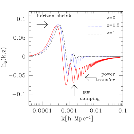
Figure 1: Redshift evolution of the function $h_{2}(k,z)$ for the fiducial cosmological model with $\Omega_{m}=0.3$ and $\Omega_{\lambda}=0.7$. Overall scale is irrelevant here. There are three effects that change the contribution of $k$-mode to the quadrupole pattern $H_{2}(z)$. Arrows show how these effects change the shape of the curve $h_{2}(k,z)$ with increasing $z$.

We will now attempt a quantitative analyses aimed to determine which wave number $k$ provides the dominant contribution to the function $h_{l}(k,z)$. We define a function $R(z)$ that is the mean of $\log_{10}[k]$ weighted by the weight $h_{2}(k,z)^{2}$ as follows $R(z)=\frac{\int\frac{dk}{k}\log_{10}[k]~{}h_{2}(k,z)^{2}}{\int\frac{dk}{k}h_{2}(k,z)^{2}}.$ If we define $\log_{10}[k_{*}]\equiv R(z)$, the wavelength $k_{*}$ can be regarded as a typical scale probed by the moment $H_{2}(z)$. We obtained $R(0)=-3.16$, $R(0.6)=-3.42$, $R(1.0)=-3.41$ and $R(2.0)=-3.38$ (with $k$ is in units of $h{\rm Mpc^{-1}}$). Roughly speaking, we can reduce the effective wave number by a factor of $\sim 2$ by using a map at $z\sim 1$, compared with the quadrupole temperature anisotropies observed today. For the sake of comparison we also calculated the same kind of quantity for the temperature anisotropies at $z=0$, and found $R=-3.08$ ($R=-3.00$) for $l=3$ ($l=4$).

In addition to $R(z)$, we also studied the contributions of fluctuations below and above $k=10^{-3}h{\rm Mpc^{-1}}$ to the spectrum $H_{2}(z)$. In figure 1 the wave number $k=10^{-3}h{\rm Mpc^{-1}}$ is given by the vertical long-dashed line, and corresponds to $\sim 6.3h^{-1}$Gpc in real scale. At $z=0$ about $32\%$ of the power is coming from $k>10^{-3}h{\rm Mpc^{-1}}$, but its contribution decreases to $\sim 2\%$ at $z=1$. We conclude that the quadrupole of the cluster polarization signal at $z\sim 1$ would allow to probe the large scale power of the Universe in a cleaner way.

So far, we mainly discussed the quadrupole mode. As we commented earlier, we expect higher modes $(l\geq 3)$ to be generated by the spin-orbit coupling. In figure 2 we show the spectrum $H_{l}(z)$ as a function of redshift. At $z=0$ the polarization map $X$ simply reflects our local quadrupole mode so that $H_{l\geq 3}=0$. The total power $\sum_{l=2}^{\infty}H_{l}(z)$ (dashed curve) is the averaged local temperature quadrupole moment $\sum_{m}\left\langle a_{2m}a^{*}_{2m}\right\rangle$ at each redshift (see eq.(1)). At $z\gtrsim 1$ it becomes a constant value due to the scale invariance of the matter power spectrum. The quadrupole mode $H_{2}(z)$ decreases continuously with increasing redshift due to the power transfer to higher-$l$ modes. However, the $l=2$ mode remains the largest signal at redshifts $z\lesssim 2$ where the cluster polarization map would be observationally available.

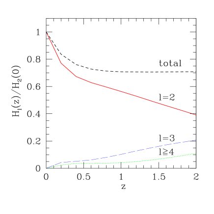
Figure 2: Redshift evolution of the spectrum $H_{l}(z)$ for parameters $\Omega_{m}=0.3$, $\Omega_{\lambda}=0.7$ and $n=1$.

We shall now consider if the redshit dependence of the polarization signal can be used to constrain cosmology. In particular we investigate possible constraints on the equation of state of dark energy. We evaluate the parameter estimation errors using the Fisher matrix approach applied to $H_{2}(z)$. We combine information on $H_{2}(z)$ from different redshift shells between $0\leq z\leq 2$ binned in $\delta z=0.2$ intervals, and assume cosmic variance with appropriate bin correlations (see eq.(6), and also Port ), as the sole source of the error.

We constrain a single fitting parameter $w=P/\rho=$constant around the fiducial model ($\Omega_{m}=0.3$, $\Omega_{\lambda}=0.7$ and $n=1$), and find $\Delta w\simeq 0.6$ ($1\sigma$). Such a large error is due to the large cosmic variance in each redshift bin and to the strong correlations between bins. Indeed the SW effect is not important for dark energy studies, but it contributes to the above correlation. Thus, in the attempt of removing the SW contribution, we also applied the Fisher matrix approach to the estimator $\sum_{m}\left\langle|b_{2m}(z)-b_{2m}(0)|^{2}\right\rangle$, and found $\Delta w\simeq 0.4$ ($1\sigma$). In order to improve this result we could also include, in principle, information of the higher order modes $l\geq 3$. In an actual observational analysis, we need a lot of efforts to detect these weak signals around at $z\lesssim 1$ where the effect of the dark energy is important (see figure 2). We conclude that cluster polarization alone would not be a powerful observational method to constrain dark energy.

Finally let us make an order of magnitude estimate for observational requirement needed to measure the moment $H_{2}(z)$ at $z\sim 1$ (see also Cooray:2003hd ). Suppose we measure the polarization signal for $N$ clusters distributed on the whole sky at $z\sim 1$ with an observational error $\sigma$ on the polarization intensity for each cluster. The total error for $H_{l}$ is $\Delta H_{l}=\sqrt{2(2l+1)}[H_{l}/(2l+1)+4\pi\sigma^{2}/N]$ with the first term representing the cosmic variance and the second term being the measurement error. For $l=2$ the two errors are equal if $\sigma\sim 0.3(\tau_{c}/10^{-2})(N/10^{3})^{1/2}\mu$K. A part from the sensitivity considerations, there is also the issue of separating the cluster polarization signal from the other competing ones, like, for example, the CMB lensing. This is best achieved if the cluster is spatially resolved, which typically requires observations with resolution of $\sim 1$ arcmin. Planck, for example, is an all sky survey mission with sensitivity $\sim 5\mu$K per pixel (for combined polarization channels and 14 months integration) and $\sim 5$ arcmin angular resolution. Because of the low resolution, it may not be the most suited experiment to detect $H_{2}$ around $z\sim 1$.

As the polarization pattern is dominated by the low-$l$ modes, a fine sky sampling is not necessary to map it. Furthermore, in order to probe only $l=2$ mode at $z\lesssim 1$ where $l\geq 3$ modes are weak, we just need to observe half of the sky ($2\pi$[sr]) due to the parity symmetry of scalar perturbations (though, in this case, the power transfer in figure 1 does not work). A ground–based telescope performing targeted cluster observations in small areas sparsely distributed on half sky may be an adequate tool to achieve this task.

The authors would like to thank A. Cooray and M. Sasaki for discussions. N.S. is supported by NASA grant NNG04GK98G and the Japan Society for the Promotion of Science. E.P. is an ADVANCE fellow (NSF grant AST-0340648) and also supported by NASA grant NAG5-11489.

References

- (1) C. L. Bennett et al., Astrophys. J. Suppl. 148, 1 (2003).
- (2) D. N. Spergel et al., Astrophys. J. Suppl. 148, 175 (2003).
- (3) M. Tegmark, et al., Phys. Rev. D 68, 123523 (2003); G. Efstathiou, Mon. Not. Roy. Astron. Soc. 346, L26 (2003); I. J. O’Dwyer et al., Astrophys. J. 617, L99 (2004).
- (4) A. de Oliveira-Costa, M. Tegmark, M. Zaldarriaga and A. Hamilton, Phys. Rev. D 69, 063516 (2004);
- (5) N. J. Cornish et al., Phys. Rev. Lett. 92, 201302 (2004).
- (6) C. R. Contaldi et al., JCAP 0307, 002 (2003).
- (7) M. Zaldarriaga, D. N. Spergel and U. Seljak, Astrophys. J. 488, 1 (1997); O. Dore, G. P. Holder and A. Loeb, Astrophys. J. 612, 81 (2004).
- (8) C. Skordis and J. Silk, arXiv:astro-ph/0402474.
- (9) M. Kamionkowski and A. Loeb, Phys. Rev. D 56, 4511 (1997).
- (10) D. Baumann and A. Cooray, New Astron. Rev. 47, 839 (2003).
- (11) A. Cooray, et al., Phys. Rev. D 69, 027301 (2004).
- (12) J. Portsmouth, Phys. Rev. D 70, 063504 (2004).
- (13) N. Seto and M. Sasaki, Phys. Rev. D 62, 123004 (2000); A. Amblard and M. J. White, arXiv:astro-ph/0409063.
- (14) W. Hu and M. J. White, Phys. Rev. D 56, 596 (1997).
- (15) M. Zaldarriaga and U. Seljak, Phys. Rev. D 55, 1830 (1997); M. Kamionkowski, A. Kosowsky and A. Stebbins, Phys. Rev. D 55, 7368 (1997).
- (16) K. Gorski, Astrophys. J. 332, L7 (1988).
- (17) P. G. Castro, A. F. Heavens and T. D. Kitching, arXiv:astro-ph/0503479.
- (18) J. J. Sakurai, Modern Quantum Mechanics (Addison-Wesley, New York, 1985).