Dip in UHECR spectrum as signature of proton interaction with CMB

Abstract

Ultrahigh energy (UHE) extragalactic protons propagating through cosmic microwave radiation (CMB) acquire the spectrum features in the form of the dip, bump (pile-up protons) and the Greisen-Zatsepin-Kuzmin (GZK) cutoff. We have performed the analysis of these features in terms of the modification factor. This analysis is weakly model-dependent, especially in case of the dip. The energy shape of the dip is confirmed by the Akeno-AGASA data with $\chi^{2}=19.06$ for $\mbox{d.o.f.}=17$ with two free parameters used for comparison. The agreement with HiRes data is also very good. This is the strong evidence that UHE cosmic rays observed at energies $1\times 10^{18}$ eV – $4\times 10^{19}$ eV are extragalactic protons propagating through CMB. The dip is also present in case of diffusive propagation in magnetic field.

, and

1 Introduction

The nature of signal carriers of UHECR is not yet established. The most natural primary particles are extragalactic protons. Due to interaction with the CMB radiation the UHE protons from extragalactic sources are predicted to have a sharp steepening of energy spectrum, so called GZK cutoff [1].

There are two other signatures of extragalactic protons in the spectrum: dip and bump [2, 3, 4, 5]. The dip is produced due to $p+\gamma_{\rm CMB}\to p+e^{+}+e^{-}$ interaction at energy centered by $E\approx 8\times 10^{18}$ eV. The bump is produced by pile-up protons which loose energy in the GZK cutoff. As was demonstrated in [3], see also [5], the bump is clearly seen from a single source at large redshift $z$, but it practically disappears in the diffuse spectrum, because individual peaks are located at different energies.

As will be discussed in this paper, the dip is a reliable feature in the UHE proton spectrum (see also [6] - [8]). Being relatively faint feature, it is however clearly seen in the spectra observed by AGASA, Fly’s Eye, HiRes and Yakutsk arrays (see [9] and [10] for the data). We argue here that it can be considered as the confirmed signature of interaction of extragalactic UHE protons with CMB.

Figure 1: The HiRes data [11] on mass composition. The measured atmospheric depths of EAS maximum $X_{\rm max}$ at $E\geq 1\times 10^{18}$ eV (triangles) are in a good agreement with QGSJet-Corsika prediction for protons.

The measurement of the atmospheric height of EAS maximum, $X_{\rm max}$, in the HiRes experiment (see Fig.1) gives another evidence of the proton composition of UHECR at $E\geq 1\times 10^{18}$ eV. Yakutsk [12] and HiRes-Mia [13] data also favour the proton composition at $E\geq 1\times 10^{18}$ eV, though some other methods of mass measurements indicate the mixed chemical composition [14].

At what energy the extragalactic component sets in?

According to the KASCADE data [15], the spectrum of galactic protons has a steepening at $E\approx 2.5\times 10^{15}$ eV (the first knee), helium nuclei - at $E\approx 6\times 10^{15}$ eV, and carbon nuclei - at $E\approx 1.5\times 10^{16}$ eV. It confirms the rigidity-dependent confinement with critical rigidity $R_{c}=E_{c}/Z\approx 3\times 10^{15}$ eV. Then CR galactic iron nuclei are expected to have the critical energy of confinement at $E_{c}\sim 1\times 10^{17}$ eV, and extragalactic protons can naturally dominate at $E\geq 1\times 10^{18}$ eV. This energy is close to the position of the second knee (Akeno - $6\times 10^{17}$ eV, Fly’s Eye - $4\times 10^{17}$ eV, HiRes - $7\times 10^{17}$ eV and Yakutsk - $8\times 10^{17}$ eV). The detailed analysis of transition from galactic to extragalactic component of cosmic rays is given in [16]. It favours the transition at $E\sim 1\times 10^{18}$ eV. The model of galactic cosmic rays developed by Biermann et al [17] also predicts the second knee as the ”end” of galactic cosmic rays due to rigidity bending in wind-shell around SN, produced by Wolf-Rayet stars. The extragalactic component becomes the dominant one at energy $E\sim 1\times 10^{18}$ eV (see Fig.1 in [17]).

Below we shall analyze the features in UHE proton spectrum using basically two assumptions: the uniform distribution of the sources in the universe and the power-law generation spectrum. We shall discuss how large-scale inhomogeneities in source distribution affect the shape of the features. We do not consider the possible speculations, such as cosmological evolution of sources. In contrast to our earlier works [6, 7, 16], we do not use here the model-dependent complex generation spectrum: the modification factor method allows us to use more general power-law spectrum with an arbitrary $\gamma_{g}$.

2 Bump in the diffuse spectrum

The analysis of the bump and dip is convenient to perform in terms of modification factor [3].

The modification factor is defined as a ratio of the spectrum $J_{p}(E)$, with all energy losses taken into account, to unmodified spectrum $J_{p}^{\rm unm}$, where only adiabatic energy losses (red shift) are included,

$$\eta(E)=J_{p}(E)/J_{p}^{\rm unm}(E).$$ (1)

For the power-law generation spectrum $\propto E_{g}^{-\gamma_{g}}$ from the sources without cosmological evolution one obtains the unmodified spectrum as

$$J_{p}^{\rm unm}(E)=\frac{c}{4\pi}(\gamma_{g}-2){\mathcal{L}}_{0}E^{-\gamma_{g}}\int_{0}^{z_{\rm max}}dz\frac{dt}{dz}(1+z)^{-\gamma_{g}+1},$$ (2)

where the observed energy $E$ and emissivity ${\mathcal{L}}_{0}$ are measured in GeV and GeV/Mpc³yr, respectively. The connection between $dt$ and $dz$ is given by usual cosmological expression (see e.g. [7]). The flux $J_{p}(E)$ is calculated as in [6] with all energy losses included.

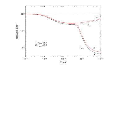
Figure 2: Modification factor for the power-law generation spectra with $\gamma_{g}$ in the range 2.0 - 2.7. Curve $\eta=1$ corresponds to adiabatic energy losses, curves $\eta_{ee}$ - to adiabatic and pair production energy losses and curves $\eta_{\rm tot}$  -  to all energy losses.

In Fig. 2 the modification factor is shown as a function of energy for two spectrum indices $\gamma_{g}=2.0$ and $\gamma_{g}=2.7$. They do not differ much from each other because both numerator and denominator in Eq. (1) include factor $E^{-\gamma_{g}}$. Let us discuss first the bump. We see no indication of the bump in Fig. 2 at merging of $\eta_{ee}(E)$ and $\eta_{\rm tot}(E)$ curves, where it should be located. The absence of the bump in the diffuse spectrum can be easily understood. The bumps are clearly seen in the spectra of the single remote sources [3]. These bumps, located at different energies, produce a flat feature, when they are summed up in the diffuse spectrum. This effect can be illustrated by Fig. 5 from Ref. [3]. The diffuse flux there is calculated in the model where sources are distributed uniformly in the sphere of radius $R_{\rm max}$ (or $z_{\rm max}$). When $z_{\rm max}$ are small (between 0.01 and 0.1) the bumps are seen in the diffuse spectra. When radius of the sphere becomes larger, the bumps merge producing the flat feature in the spectrum. If the diffuse spectrum is plotted as $E^{3}J_{p}(E)$ this flat feature looks like a pseudo-bump.

3 Dip as a signature of the proton interaction with CMB.

The dip is more reliable signature of interaction of protons with CMB than GZK feature. The shape of the GZK feature is strongly model-dependent: it is more flat in case of local overdensity of the sources, and more steep in case of their local deficit. It depends also on fluctuations in the distances between sources inside the GZK sphere and on fluctuations of luminosities of the sources there.

Figure 3: Predicted dip in comparison with the Akeno-AGASA data.

The shape of the dip is fixed and has a specific form which is difficult to imitate by other mechanisms. The protons in the dip are collected from the large volume with the radius about 1000 Mpc and therefore the assumption of uniform distribution of sources within this volume is well justified. In contrast to this well predicted and specifically shaped feature, the cutoff, if discovered, can be produced as the acceleration cutoff. Since the shape of both GZK cutoff and acceleration cutoff is model-dependent, it will be difficult to argue in favour of any of them. The problem of identification of the dip depends on the accuracy of observational data, which should confirm the specific (and well predicted) shape of this feature. Do the present data have the needed accuracy?

The comparison of the calculated modification factor with that obtained from the Akeno-AGASA data, using $\gamma_{g}=2.7$, is given in Fig. 3. It shows the excellent agreement between predicted and observed modification factors for the dip.

In Fig. 3 one observes that at $E<1\times 10^{18}$ eV the agreement between calculated and observed modification factors becomes worse and at $E\leq 4\times 10^{17}$ eV the observational modification factor becomes larger than 1. Since by definition $\eta(E)\leq 1$, it signals about appearance of another component of cosmic rays, which is most probably galactic cosmic rays. The condition $\eta>1$ means the dominance of the new (galactic) component, the transition occurs at higher energy.

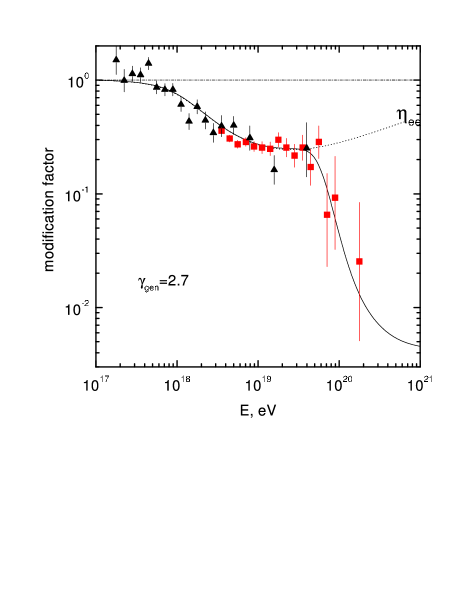
Figure 4: Predicted dip in comparison with the HiRes data.

To calculate $\chi^{2}$ for the confirmation of the dip by Akeno-AGASA data, we choose the energy interval between $1\times 10^{18}$ eV (which is somewhat arbitrary in our analysis) and $4\times 10^{19}$ eV (the energy of intersection of $\eta_{ee}(E)$ and $\eta_{\rm tot}(E)$). In calculations we used the Gaussian statistics for low-energy bins, and the Poisson statistics for the high energy bins of AGASA. It results in $\chi^{2}=19.06$. The number of Akeno-AGASA bins is 19. We use in calculations two free parameters: $\gamma_{g}$ and the total normalization of spectrum. In effect, the confirmation of the dip is characterised by $\chi^{2}=19.06$ for d.o.f.=17, or $\chi^{2}$/d.o.f.=1.12, very close to the ideal value 1.0 for the Poisson statistics.

In Fig. 4 the comparison of modification factor with the HiRes data is shown. The agreement is also very good: $\chi^{2}=19.5$ for $d.o.f.=19$ for the Poisson statistics.

The good agreement of the shape of the dip $\eta_{ee}(E)$ with observations is a strong evidence for extragalactic protons interacting with CMB. This evidence is confirmed by the HiRes data on the mass composition (see Fig. 1).

The dip is also present in case of diffusive propagation in magnetic field [18].

4 Extragalactic iron nuclei as UHECR primaries

Does modification factor for iron nuclei differ from the proton dip?

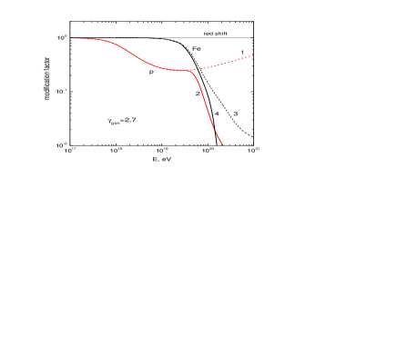
Figure 5: Modification factor for iron nuclei in comparison with that for protons. Curve $\eta=1$ corresponds to adiabatic energy losses. Proton modification factors are given given by curve 1 (adiabatic and pair production energy losses) and by curve 2 (total energy losses). Iron modification factors are given by curve 3 (adiabatic and pair production energy losses) and by curve 4 (with photodissociation included).

We calculated the modification factor for iron nuclei, assuming that that Fe nuclei are the heaviest ones accelerated in the sources, and considering the propagation of Fe nuclei with energy losses taken into account. The resulting flux is given only for primary iron nuclei, without secondary nuclei produced during propagation (more details will be presented in [19]).

The energy losses for Fe are dominated by adiabatic energy losses up to $4.5\times 10^{19}$ eV, from where on $e^{+}e^{-}$ energy losses dominate. For energies $E\geq 1.7\times 10^{20}$ eV photodissociation becomes the main source of energy losses [21, 19]. According to this dependence the energy spectrum of iron nuclei is $\propto E^{-\gamma_{g}}$ up to $E_{1}\sim 1\times 10^{19}$ eV, where the first steepening begins. The second steepening, caused by iron-nuclei destruction, occurs at energy $E_{2}\sim 1\times 10^{20}$ eV. For lighter nuclei the steepening (cutoff) starts at lower energies. Therefore the cutoff of the nuclei spectra occurs approximately at the same energy as the GZK cutoff, though the physical reason for these two cutoffs is different: while the latter (GZK) is caused by starting of photopion production, the former (nuclei) - by transition from adiabatic to pair-production energy losses [20].

In Fig. 5 the modification factors for iron nuclei are shown as function of energy in comparison with modification factors for protons. Comparison with Fig. 3 clearly shows that even small admixture of iron nuclei in the primary extragalactic flux upsets the good agreement of the proton dip with observational data.

5 Discussion and conclusions

There are three signatures of UHE protons propagating through CMB: GZK cutoff, bump and dip.

The energy shape of the GZK feature is model dependent. The local excess of sources makes it flatter, and the deficit - steeper. The shape is affected by fluctuations of source luminosities and distances between the sources. The cutoff, if discovered, can be produced as the acceleration cutoff (steepening below the maximum energy of acceleration). Since the shape of both, the GZK cutoff and acceleration cutoff, is model-dependent, it will be difficult to argue in favour of any of them, in case a cutoff is discovered.

The bump is produced by pile-up protons, which are loosing energy in photopion interactions and are accumulated at low energy, where the photopion energy losses become equal to that due to pair-production. Such bump is distinctly seen in calculation of spectrum from a single remote source. In the diffuse spectrum, since the individual peaks located at different energies, a flat spectrum feature is produced.

The dip is the most remarkable feature of interaction with CMB. The protons in this energy region are collected from the distances $\sim 1000$ Mpc, with each radial interval $dr$ providing the equal flux. All density irregularities and all fluctuations are averaged at this distance, and assumption of uniform distribution of sources with average distances between sources and average luminosities becomes quite reliable. The dip is confirmed by Akeno-AGASA and HiRes data with the great accuracy (see Figs 3 and 4). As one can see from Fig. 5, presence of even small fraction of extragalactic heavy nuclei in the primary flux upsets this agreement.
We interpret the excellent agreement of the calculated dip with the observations as an independent evidence that observed primaries at energy $1\times 10^{18}-4\times 10^{19}$ eV are extragalactic protons. This evidence is the complementary one to the direct measurements (now contradictive) of chemical composition.
At energy $E<4\times 10^{17}$ eV the modification factor from Akeno data exceeds 1, and it signals about dominance of another cosmic ray component, most probably the galactic one. It agrees with transition from galactic to extragalactic component at the second knee $E\sim 1\times 10^{18}$ eV. This conclusion is confirmed by the recent HiRes data on mass composition (see Fig. 1) and indirectly by the KASCADE data (see [16] for the detailed analysis).

Are there alternative explanations of the dip? The conservative one (see e.g. [22]) is known since early 80s, when the spectrum feature, ankle, was discovered in the Haverah Park data [23] at $E\sim 1\times 10^{19}$ eV. This feature was interpreted as transition from galactic to extragalactic cosmic rays (in contrast to the calculations above where the ankle naturally appears as a part of the dip). The hypothesis of the transition at the ankle can be described phenomenologically as follows: At energy below $1\times 10^{19}$ eV the cosmic ray flux is galactic and above - extragalactic. The galactic spectrum can be taken basically as power-law $\propto E^{-\gamma_{\rm gal}}$, but agreement with observations needs steepening at $E\geq E_{g}$, described by some steepening parameter. In effect one can use the parametrization:

$$I_{\rm gal}(E)=K_{\rm gal}E^{-\gamma_{\rm gal}}\left[1-a\exp(b\log E/10^{19}~{}{\rm eV})\right].$$ (3)

The extragalactic generation spectrum is assumed to be power-law with index $\gamma_{g}$. Together with two constants of the normalization for both fluxes, one has as minimum six free parameters to fit the observed spectrum. We found the best fit shown in Fig. 6. It is characterized by $\chi^{2}=9.1$ for 19 energy bins and 6 free parameters, i.e. by $\chi^{2}/d.o.f.=0.7$ for d.o.f.=13. The value $\chi^{2}/d.o.f.<1$ for the Poisson statistics signals for the large number of the free parameters and for very good formal fit to the experimental data. The problem of this ad hoc model is whether there is a physical model for propagation of galactic cosmic rays, which results in spectrum given by Eq.(3). It is just assumed that the spectrum at $E<1\times 10^{19}$ eV is the same as observed, while the dip model predicts this spectrum in excellent agreement with observations. An intermediate case is given in [24] where the dip is mostly described by extragalactic protons interacting with CMB with a small correction given by galactic cosmic rays only at the low-energy, $E\approx 1\times 10^{18}$ eV, part of the dip (see Fig. 13 in [24]).

Figure 6: The ad hoc model for explanation of the dip. The distorted power-law spectrum (3) is shown by curve “galactic”. The extragalactic spectrum with $\gamma_{g}=2$ is normalized by the data in the interval $(4-6)\times 10^{19}$ eV. The parameters of the galactic spectrum are found to provide the best fit to the data by the total spectrum (galactic + extragalactic), shown by the thick curve. It gives $\gamma_{\rm gal}=3.28$.

How does extragalactic magnetic field affect the discussed spectra features?

The influence of magnetic field on spectrum depends on the separation of the sources $d$. There is a statement which has a status of the theorem [25]:
For uniform distribution of sources with separation much less than characteristic lengths of propagation, such as energy attenuation length $l_{\rm att}$ and the diffusion length $l_{\rm diff}$, the diffuse spectrum of UHECR has an universal (standard) form independent of mode of propagation.

For the realistic intergalactic magnetic fields the spectrum is universal in energy interval $1\times 10^{18}-8\times 10^{19}$ eV [18]. Note, however, that generation spectrum is defined in [25] as one outside the source. In this work we implicitly assume that the sources are transparent for UHE protons and thus the generation spectrum is the same as the acceleration spectrum.

The most probable astrophysical sources of UHECR are AGN. They can accelerate particles to $E_{\rm max}\sim 1\times 10^{21}$ eV and provide the needed emissivity of UHECR ${\mathcal{L}}_{0}\sim 3\times 10^{46}$ erg/Mpc³yr. The correlation of UHE particles with directions to special type of AGN, Bl Lacs, is found in analysis of work [26]. AGN as UHECR sources in case of quasi(rectilinear) propagation of protons explain most naturally the small-scale anisotropy [27].

The UHECR from AGN have a problem with superGZK particles with energies $E>1\times 10^{20}$ eV: (i) another component is needed for explanation of the AGASA excess, and (ii) no sources are observed in AGASA and other arrays in direction of superGZK particles. These problems probably imply the new physics, such as UHECR from superheavy dark matter, new signal carrier, like e.g. new light stable hadron, strongly interacting neutrino, and Lorentz invariance violation. For the last case it is interesting to note that if Lorentz invariance is weakly broken for $e^{+}e^{-}$ production, but strongly for pion production, then the modification factor is given by the curve $\eta_{ee}$ in Fig. 3. This prediction agrees well with the Akeno-AGASA spectrum.

References

- [1] K. Greisen, Phys. Rev. Lett., 16, 748 (1966); G. T. Zatsepin, V. A. Kuzmin, Pisma Zh. Experim. Theor. Phys. 4, 114 (1966).
- [2] C. T. Hill and D. N. Schramm, Phys. Rev. D 31, 564 (1985).
- [3] V. S. Berezinsky and S. I. Grigorieva, Astron. Astroph. 199, 1 (1988).
- [4] S. Yoshida and M. Teshima, Progr. Theor. Phys. 89, 833 (1993).
- [5] T. Stanev et al., Phys. Rev. D 62, 093005 (2000).
- [6] V. Berezinsky, A. Z. Gazizov, S. I. Grigorieva, astro-ph/0204357.
- [7] V. Berezinsky, A. Z. Gazizov, S. I. Grigorieva, astro-ph/0210095.
- [8] V. Berezinsky, A. Z. Gazizov, S. I. Grigorieva, Proc. of Int. Workshop “Extremely High-Energy Cosmic Rays” (eds M.Teshima and T. Ebisuzaki), Universal Press, Tokyo, Japan, p. 63 (2002).
- [9] M. Takeda et al. [AGASA collaboration], astro-ph/0209422; N. Hayashida et al. [AGASA collaboration], Phys. Rev. Lett. 73, 3491 (1994); K. Shinozaki et al. [AGASA collaboration], Astrophys. J. 571, L117 (2002); T. Abu-Zayyad et al. [HiRes collaboration], astro-ph/0208243; D. J. Bird et al. [Fly’s Eye collaboration], Ap. J. 424, 491 (1994); A. V. Glushkov et al. [Yakutsk collaboration] Proc. of 28th Int. Cosmic Ray Conf. (Tsukuba, Japan), 1, 389 (2003); M. Ave et al [Haverah Park collaboration], Astrop. Phys. 19, 61 (2003).
- [10] M. Nagano and A. Watson, Rev. Mod. Phys. 72, 689 (2000).
- [11] G. Archbold and P. V. Sokolsky, Proc. of 28th ICRC, 405 (2003).
- [12] A. V. Glushkov et al. (Yakutsk collaboration) JETP Lett. 71, 97 (2000).
-
[13]
T.Abu-Zayyad et al., Astrophys. J., 557, 686 (2001);
T.Abu-Zayyad et al.,Phys. Rev. Lett. 84, 4276 (2003). - [14] A. Watson, Proc. of CRIS 2004 conference (Catania 2004), astro-ph/0408110.
- [15] K.-H. Kampert et al (KASCADE collaboration) Proc. 27th ICRC, volume Invited, Rapporteur and Highlight papers, 240 (2001).
- [16] V. Berezinsky, S. Grigorieva and B. Hnatyk, Astroparticle Physics, 21, 617 (2004).
- [17] P. L. Biermann et al, 2003, astro-ph/0302201.
- [18] R. Aloisio and V. Berezinsky, astro-ph/0412578.
- [19] R. Aloisio, V. Berezinsky, S. Grigorieva, in preparation.
- [20] V. S. Berezinsky, S. I. Grigorieva, G. T. Zatsepin, Proc. 14th ICRC (Munich) 2, 711 (1975).
- [21] F. W. Stecker and M. H. Salamon, Astrophys.J. 512, 521 (1999).
-
[22]
A. M. Hillas, talk at the Leeds Cosmic Ray Conference;
T. Wibig and A. W. Wolfendale, astro-ph/0410624. - [23] G. Cunningham et al. (Haverah Park collaboration), Astroph. J. 236, L71, (1980).
- [24] S. D. Wick, C. D. Dermer, A. Atoyan , Astrop. Phys. 21, 125 (2004).
- [25] R. Aloisio and V. Berezinsky, Astroph. J., 612, 900 (2004).
- [26] P. G. Tinyakov and I. I. Tkachev, JETP Lett., 74, 445 (2001).
- [27] S. L. Dubovsky P. G. Tinyakov and I. I. Tkachev, Phys. Rev. Lett. 85, 1154 (2000); Z. Fodor and S. Katz, Phys. Rev. D63, 23002 (2001); P. Blasi and D. De Marco, Astrop. Phys. 20, 559 (2004); M. Kachelriess and D. Semikoz, astro-ph/0405258.