Characterizing a new class of variability in GRS 1915$+$105 with simultaneous INTEGRAL/RXTE observations

We report on the analysis of 100 ks INTEGRAL observations of the Galactic microquasar GRS 1915$+$105. We focus on INTEGRAL Revolution number 48 when the source was found to exhibit a new type of variability as preliminarily reported in Hannikainen et al. (2003). The variability pattern, which we name $\xi$, is characterized by a pulsing behaviour, consisting of a main pulse and a shorter, softer, and smaller amplitude precursor pulse, on a timescale of 5 minutes in the JEM-X 3–35 keV lightcurve. We also present simultaneous RXTE data. From a study of the individual RXTE/PCA pulse profiles we find that the rising phase is shorter and harder than the declining phase, which is opposite to what has been observed in other otherwise similar variability classes in this source. The position in the colour-colour diagram throughout the revolution corresponds to State A (Belloni et al. 2000) but not to any previously known variability class. We separated the INTEGRAL data into two subsets covering the maxima and minima of the pulses and fitted the resulting two broadband spectra with a hybrid thermal–non-thermal Comptonization model. The fits show the source to be in a soft state characterized by a strong disc component below $\sim$6 keV and Comptonization by both thermal and non-thermal electrons at higher energies.

1 Introduction

GRS 1915$+$105 has been extensively observed at all wavelengths ever since its discovery. It was originally detected as a hard X-ray source with the WATCH all-sky monitor on the GRANAT satellite (Castro-Tirado, Brandt & Lund 1992). Apparent superluminal ejections have been observed from GRS 1915$+$105 several times with the Very Large Array in 1994 and 1995 (Rodríguez & Mirabel 1999) and in 1997 with the Multi-Element Radio-Linked Interferometer Network (Fender et al. 1999). Both times the true ejection velocity was calculated to be $>0.9c$. In addition to these superluminal ejections at the arcsec scale, GRS 1915$+$105 has also exhibited a compact radio jet resolved at milli-arcsec scales corresponding to a length of a few tens of AU (Dhawan, Mirabel & Rodríguez 2000; Fuchs et al. 2003). Using the Very Large Telescope, Greiner et al. (2001) identified the mass-donating star to be of spectral type K-M III. The mass of the black hole was deduced by Harlaftis & Greiner (2004) to be $14.0\pm 4.4\,{\rm M}_{\odot}$ in a binary orbit with the giant star of 33.5 days. The Rossi X-ray Timing Explorer (RXTE) has observed GRS 1915$+$105 since its launch in late 1995 and has shown the source to be highly variable on all timescales from milliseconds to months (see e.g. Belloni et al. 2000; Morgan, Remillard & Greiner 1997). Belloni et al. (2000) categorized the variability into twelve distinct classes which they labelled with Greek letters (two of those represented by semi-regular pulsing behaviour), and identified three distinct X-ray states: two softer states, A and B, and a harder state, C. The source has been detected up to $\sim$ 700 keV during OSSE observations (Zdziarski et al. 2001). For a recent comprehensive review of GRS 1915$+$105 see Fender & Belloni (2004).
The European Space Agency’s INTErnational Gamma-Ray Astrophysical Laboratory (INTEGRAL) is aimed at observing the sky between $\sim$ 3 keV and 10 MeV (Winkler et al. 2003). The INTEGRAL payload consists of two gamma-ray instruments – the Imager on Board the INTEGRAL Spacecraft, IBIS (Ubertini et al. 2003), and the Spectrometer on INTEGRAL, SPI (Vedrenne et al. 2003); two identical X-ray monitors – the Joint European X-ray monitor, JEM-X (Lund et al. 2003); and an optical monitor (Mas-Hesse et al. 2003).
GRS 1915$+$105 is being observed with INTEGRAL as part of the Core Program and also within the framework of an Open Time monitoring campaign. Here we present the results of the first of our AO-1 Open Time observations which took place during INTEGRAL Revolution number 48. The source was found to exhibit a new type of variability not documented in Belloni et al. (2000). Preliminary results were described elsewhere (Hannikainen et al. 2003). We also have a simultaneous observing campaign with RXTE to concentrate on timing analysis (Rodriguez et al. 2004a). The main goal of this INTEGRAL/RXTE program was to study the disc-jet connection in GRS 1915$+$105 and to study the variability classes in the hard X-ray regime. As the source behaviour is very unpredictable, we were not able to study the disc-jet connection in this particular case, nor any of the already known variability classes. Instead, (as we show below), the source exhibited a new type of variability and we discovered a new source (IGR J19140$+$0951) during the observation. In this paper, we conduct a more detailed analysis of the high energy behaviour of GRS 1915$+$105 during Revolution 48. In Section 2 we discuss the observation and data reduction methods, while in Section 3 we re-introduce the new type of variability. In Section 4 we present the RXTE results, while in Section 5 we discuss the spectral analysis of the INTEGRAL data. Finally, in Section 6 we present a summary of the paper.

2 Observations and data reduction

As part of a monitoring programme which consists of six 100-ks observations, INTEGRAL observed GRS 1915$+$105 for the first time for this campaign on 2003 Mar 6 beginning at UT 03:22:33 during INTEGRAL’s Revolution 48 for 100 ks. The INTEGRAL observations were undertaken using the hexagonal dither pattern (Courvoisier et al. 2003), which consists of seven pointings around a nominal target location (1 source on-axis pointing, 6 off-source pointings, each $2^{\circ}$ apart, with each science window of 2200 s duration). This means that GRS 1915$+$105 was always in the field-of-view of all three X-ray and gamma-ray instruments (JEM-X, IBIS and SPI) throughout the whole observation.
Figure 1 shows the RXTE/ASM one-day average 1.3–12 keV lightcurve. The vertical line indicates the date of the INTEGRAL and the simultaneous RXTE pointed observations.

Figure 1: The RXTE/ASM one-day average 1.3–12 keV lightcurve showing the epoch of the INTEGRAL observation and the simultaneous pointed RXTE observation (dashed line).

2.1 INTEGRAL data reduction

All data were reduced using the Off-line Scientific Analysis (OSA) version 4.0 software. The JEM-X data were reduced following the standard procedure described in the JEM-X cookbook. Based on the JEM-X 3–35 keV lightcurve first presented in Hannikainen et al. (2003) and reproduced here (Fig. 2), we defined Good Time Intervals (GTIs) for the spectral extraction process. We created two GTI files: one for data below 70 counts s^-1 (which corresponds to $\sim$ 0.5 Crab in that energy range) and one for data above 70 counts s^-1. We then ran the analysis using the two GTI files from which we extracted two total spectra. For the modelling of the spectra, we ignored data above 30 keV for the spectrum of the bright parts and above 25 keV for the faint parts. We assumed systematic uncertainties as shown in Table 1 (P. Kretschmar & S. Martínez Núñez, priv. comm.).

Channel	Energy	Systematic uncertainty
	(keV)	(%)
$<$ 72	$<$ 5.12	10
72–79	5.12–5.76	5
80–89	5.76–6.56	2
90–99	6.56–7.36	7
100–109	7.36–8.16	5
110–119	8.16–9.12	4
120–129	9.12–10.24	5
130–149	10.24–13.44	4
150–159	13.44–15.04	6
160–169	15.04–17.64	5
170–179	17.64–20.24	8
180–189	20.24–22.84	7
190–199	22.84–26.24	9
200–209	26.24–29.84	15

Table 1: Level of systematic uncertainty applied to the spectral channels of the JEM-X spectra, and energy channel correspondence.

Figure 2: The JEM-X 3–35 keV lightcurve for the whole of Revolution 48. The time bin is 8 s. As can be seen, the source varied between $\sim$ 0.25–2 Crab. Reproduced from Hannikainen et al. (2003). Shown on the plot is our simultaneous RXTE coverage.

Concerning IBIS, we reduced the data from the top layer plane detector, ISGRI (Lebrun et al. 2003). We made a run of the software up to the IMA level, i.e. the production of images. During the run we extracted images from individual science windows in two energy ranges (20–40 keV and 40–80 keV) as well as a mosaic in the same energy ranges. As with JEM-X, the GTIs were given as input to OSA to extract the ISGRI spectral products. Rather than using the standard spectral extraction, we then re-ran the analysis software up to the IMA level in ten energy bands and then estimated the spectra. The source count rate and error were then extracted from each mosaic at the position of the source, from the intensity and variance map respectively (see the Appendix in Rodriguez et al. 2004b for an in-depth description of this method). We further assumed 8% systematics in each channel (e.g. Cadolle-Bel et al. 2004).
To reduce SPI data a pre-release version of OSA 4.0 was used, which incorporates two different analysis methods: The default pipeline is optimised for speed, but cannot handle user defined GTIs (Knödlseder et al. 2004). Hence the alternative pipeline, which is more closely based on the OSA 3 release, was adopted but using the more recent calibration data from OSA 4.0. The background flux was estimated using the Mean Count Modulation (MCM) method and spectra were extracted from the reduced data, using the same input catalogue as the ISGRI analysis, with SPIROS v8.0.1 (Skinner & McConnell 2003).

The combined JEM-X, ISGRI and SPI spectra resulted in two broadband spectra: one for the high part of the JEM-X lightcurve, which we will refer to as pulse maxima and one for the low part, corresponding to the combined pulse minima. These two spectra are used for the broadband modelling in Section 5.

2.2 RXTE data reduction

During the last third of the INTEGRAL observations we obtained simultaneous RXTE observations ($\sim 32$ ks). We reduced and analysed the data from the RXTE Proportional Counter Array using the LHEASOFT package v5.3, following the standard steps explained in the PCA cookbook; see Rodriguez, Corbel & Tomsick (2003) for the details of the selection criteria. We first extracted a 1-s resolution lightcurve between 2.5–15 keV from the binned data, from all available Proportional Counter Units (PCU) turned on during individual $\sim 90$ min RXTE revolutions. The background-corrected lightcurve is shown in Fig. 3. Since we were interested in studying the spectral variations of the source during this observation, we took advantage of the high sensitivity of the PCA to extract spectra on the smallest timescale allowed by the standard 2 data. In a manner similar to a previous work (Rodriguez et al. 2002), we extracted PCA spectra and background spectra every 16 s from the top layer of PCU 0 and 2. The responses were generated with pcarsp (V10.1). The resulting 16-s RXTE spectra are used to study fast spectral variability in Section 4.

Figure 3: a The RXTE/PCA 2.5–15 keV lightcurve (with time bin of 1 second) extracted from all PCU and layers. The observations start on MJD 52704.99. Marked in the plot are the times of the pulses dealt with in Figs. 4, 5, 6, 8 and in Section 4. Each segment in the lightcurve represents one RXTE orbit. b An expanded plot of the pulses.

3 A new type of variability?

Fig. 2 shows the entire JEM-X 100 ks lightcurve. Throughout most of the lightcurve (the high fast flaring parts, e.g. from MJD 52704.15–52704.41) we see a novel class of variability, characterized by 5-minute pulses, not observed before (Hannikainen et al. 2003). The entire JEM-X lightcurve is dominated by these 5-minute pulses, as evidenced by the 3 mHz quasi-periodic oscillation which resulted from a Fourier transform the whole JEM-X lightcurve (Hannikainen et al. 2003). Although this kind of pulsed variability resembles the $\rho$-heartbeat and $\kappa$ oscillations described in Belloni et al. (2000), the oscillations presented there are more uniform and occur on shorter timescales. In Hannikainen et al. (2003), we also produced a colour-colour diagram for the RXTE data in the same manner as in Belloni et al. (2000) and showed that the data points fell in a different part of the colour-colour diagram as compared to the other classes. We call this new type of variability $\xi$.

Figure 4: The JEM-X colour-intensity diagram from the whole 100 ks observation. The colour was constructed from the 10–35 keV and 3–10 keV lightcurves. The maxima of the flares are in the right-hand edge of the plot, while the minima are in the left-hand edge. This confirms that the rising phases are harder than the declining phases. Each point is one time bin (10 s) and represents the averaged mean value from the 300 JEM-X flares; the cross shows the average standard deviation for the mean value of each individual point throughout the loop – this includes both the variability within each point and the error (i.e. it is not an error bar).

To study the behaviour of the source in this new variability class, we produced a colour-intensity diagram from the whole 100 ks JEM-X lightcurve (Fig. 4). The JEM-X colour was constructed from the 3–10 keV and 10–35 keV lightcurves. Each point is one time bin of 10 s and represents the averaged mean value from 300 JEM-X pulses. Points from the pulse-maxima are situated in the right-hand side of the plot, while points from the minima are on the left-hand side. Indicated in the figure are the rising and declining phases of the pulses. The cross shows the standard deviation of the mean value of each point – this includes both the real variability and the error, and hence is not an error bar in the conventional sense. The figure shows not a simple flux-hardness correlation, but rather some kind of limit cycle/hysteretic behaviour with the rising phases being harder than the declining phases. This is opposite to what has been observed in other similar classes (e.g. class $\rho$). In the next section, using the RXTE data, we take a more detailed look at this behaviour, starting with an examination of the individual pulses.

4 Pulses and variability in the RXTE data

During some of the RXTE pointings, the 5-minute pulses are clearly detected also by RXTE/PCA (Fig. 3a). In one segment in particular (Fig. 3b) we see nine consecutive pulses, representative of the variability pattern in the majority of the JEM-X lightcurve. Because of the better temporal resolution and higher collecting area of RXTE/PCA compared to INTEGRAL/JEM-X, we can study the variability of the source on a timescale of 1 s with good enough statistics. This time bin is appropriate because Belloni et al. (2000) used a time bin of 1 s to make their colour-colour diagrams, hence allowing for a direct comparison between this work and theirs. Another reason why a 1-s binning was chosen is that it is not of too high resolution, and therefore does not eliminate too many points which would render the plot unclear, but at the same time is not so low so as to smear out any variability present. The RXTE/PCA lightcurve was divided into three energy bands (2–5, 5–13, and 13–40 keV) and smoothed with a boxcar average of 5 time bins. Figure 5 shows the mean of the nine RXTE/PCA pulses from Fig. 3b. The pulses consist of the main pulse (with the rising phase being shorter and harder than the declining phase) and a precursor pulse, which is shorter, softer and of smaller amplitude than the main pulse.

The times of the maxima of the 2–5 keV pulses were determined from the smoothed lightcurve. The eight latter pulses were shifted onto the first pulse using the times of the maxima as the reference. This was repeated for the other two energy bands, using the times of the maxima of the 2–5 keV pulses. From the resulting average pulse shape, we can confirm that the rising phase of the (main) pulse is harder than the declining phase. In addition, the rise is also shorter than the decline. In each of these nine pulses, there is also a precursor seen only in the softer X-ray bands.

Figure 5: The mean of nine RXTE/PCA pulses – the times covered by these nine pulses is shown in Figs. 3 and 7. The top (red) line shows the 2–5 keV lightcurve, the middle (cyan) the 5–13 keV and the bottom (blue) the 13–40 keV lighcurve. The rising phases are shorter and harder than the declining phases. The latter eight pulses were shifted onto the first pulse as described in the text, using the maximum of the 2–5 keV lightcurve as the reference point.

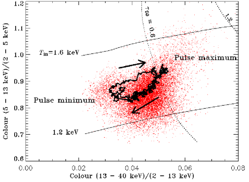
Figure 6: Colour-colour diagram showing the the RXTE/PCA from this study. The dots represent the whole observation, while the solid line superposed is from the pulses (Fig. 3b). The curved dotted lines correspond to the colours expected from a Comptonizing spherical corona with a given radial optical depth $\tau_{50}$ (i.e. optical depth for the assumed electron temperature of 50 keV) and varying values of the inner disc temperature $T_{\rm in}$. The solid lines show the colours expected for the model for given $T_{\rm in}$ and varying $\tau_{50}$. The pulse cycle goes clockwise.

To further study the indicated limit cycle, we constructed a colour-colour diagram from the RXTE/PCA data, shown in Figure 6. The X-ray colours were defined as HR1 = B/A and HR2 = C/(A + B), where A, B, and C are the counts in the 2–5 keV, 5–13 keV and 13–40 keV, respectively, following Belloni et al. (1997). In Fig. 6, the dots represent the whole RXTE observation (including the non-pulsed part), while the solid line shows the cycle traced by the pulses (Fig. 3b). The main aim of the figure is to show the small range of variability of the 5-minute pulses. The pulse cycle goes clockwise as indicated by the arrows. The maxima of the pulses are at the upper-right of the pulse cycle curve, while the minima are at the lower left.

Superposed in Fig. 6 are model curves from a study by Vilhu & Nevalainen (1998), calculated as explained below. Although a direct comparison of the parameters is not possible due to the RXTE/PCA gain evolution through the years, resulting in a change of the energy channel correspondence, we simply want to illustrate qualitatively the position in the colour-colour diagram of this present observation. In order to have an idea of what physical parameters the observed colours correspond to, we simulated the colours predicted by a Comptonization model. We assumed the Comptonizing source to be a sphere surrounded by a cooler disc with the inner radius equal to that of the sphere (Poutanen, Krolik, & Ryde 1997). Seed photons coming from the disc are characterized by the inner disc temperature $T_{\rm in}$. The electrons in the cloud were assumed to be thermal with temperature $kT=50$ keV. The Thomson optical depth of the cloud along the radius is $\tau_{50}$, with subscript 50 meaning that this $\tau$ corresponds to the 50 keV electrons. For a different $T$, similar Comptonization spectra are produced by a cloud of optical depth $\tau=\tau_{50}\times 50{\rm keV}/kT$, because the slope of the Comptonization spectrum, $\Gamma$, is a function of the Kompaneets parameter, $y=4\tau kT/m_{e}c^{2}$, and $\Gamma=\frac{9}{4}y^{-2/9}$ (Beloborodov 1999). For the given $T_{\rm in}$ and $\tau_{50}$, we compute the Comptonization spectrum using the method of Poutanen & Svensson (1996). Then we obtain the colours expected from the model spectrum using the responses of RXTE/PCA and plot them on the colour-colour diagram (Fig. 6). We see that the pulses discussed in this paper correspond to optical depth $\tau\la 0.7$ and inner disc temperature of $T_{\rm in}\sim 1.3-1.4$ keV. This temperature differs slightly from that obtained using a black body $+$ power law model, because the Comptonization spectrum is not a power law close to the seed photon energies (see e.g. Vilhu et al. 2001).

4.1 Hysteresis or limit-cycle oscillations?

Figure 7: The results from the RXTE spectral analysis. Each column represents one RXTE orbit – the fourth column from the left is from the time of the pulses examined in more detail. The top row reproduces the PCA 2–20 keV flux. The second row from the top shows the evolution of the photon index $\Gamma$ throughout the observations, the third row shows the inner disc temperature (keV), while the bottom row shows the inner disc radius (km). All results are from the fits to the 16-s spectra. Bad fits, i.e. data points with $\chi^{2}>50$ (for $\sim 41$ d.o.f.), were removed. The remaining data and fit results were smoothed with a boxcar average of 5 time bins to show the general trend throughout the data sets.

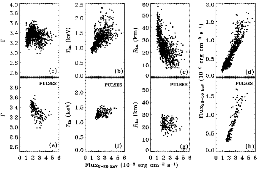
Figure 8: Panels a –d show $\Gamma$, $T_{\rm in}$, $R_{\rm in}$ and the 20–50 keV flux against the 2–20 keV flux from the whole set of the RXTE/PCA observations, while panels e–h show the same but only for the pulses.

The colour-intensity diagram in Fig. 4 and the colour-colour diagram in Fig. 6 both show loop-like features, which could be due to a hysteretic process or limit-cycle oscillations. The hysteresis phenomenon has been suggested to explain the loop features in the X-ray colour-colour diagram of black hole low-mass X-ray binaries (Miyamoto et al. 1995). One recent example is GX 339$-$4 (see Zdziarski et al. 2004). Hysteresis can occur on a large range of timescales, and for accreting black holes the timescale is attributed to the finite time required in the building up and dissipation of a viscous, optically thick accretion disc. The accretion disc gives rise to low-energy photons, which act as coolants for the hot plasma via inverse Comptonization. During the accretion disc build-up process, the source luminosity increases but the X-ray spectrum softens. On the other hand, when the accretion disc dissipates (e.g. due to evaporation), the source luminosity decreases and the X-ray spectrum hardens. The process is expected to occur in an extended region at a substantial distance from the central black hole. The duration of the two hysteretic states and their transition times are long, and for low-mass X-ray binaries the timescale would be a year or more.

In GRS 1915$+$105, the timescale for developing the loop features is relatively short – roughly hundreds of seconds. The observation is not consistent with the scenario requiring an extended accretion disc, the building up and the recession of which drive the hysteretic cycle. One may argue that the process could occur in a smaller inner disc region, and this naturally shortens the corresponding timescales. When we examined the loop in Fig. 4, we find spectral hardening accompanied by an increase in the X-ray photon counts, contrary to the properties of the hysteresis model for the GX 339$-$4 behaviour. We therefore conclude that the processes behind the loops in the colour-colour diagrams of GRS 1915$+$105 and GX 339$-$4 are not identical. As an alternative, we interpret the loops in the GRS 1915$+$105 data as limit-cycle oscillations, which are probably due to delayed feedback in the inner accretion disc. A possible explanation for the simultaneous rise in the photon counts and spectral hardening is an increase in the size of the hard X-ray emission region which produces the Comptonized hard X-rays. This region could be a hot disc corona or some non-thermal plasmas in the vicinity of the accreting black hole.

4.2 Fast spectral variability

To track variability on short timescales, the 16-s PCA spectra were fitted individually in XSPEC V11.3 (Arnaud 1996) with a simple model of absorbed power law plus multicolour disc blackbody (MCD, Mitsuda et al. 1984), and a Gaussian. The absorption column density $N_{\rm H}$ was fixed at $5\times 10^{22}$ cm^-2. The power law photon index $\Gamma$, inner disc temperature $kT_{\rm in}$ and inner disc radius $R_{\rm in}$ are plotted in Fig. 7, in addition to the actual lightcurve in flux units. All bad fits (points with $\chi^{2}>50$ for $\sim 41$ d.o.f.) were removed and the data were smoothed with a boxcar average of 5 time bins to highlight the general trend in the data sets. We clearly see amplitude variations of the fit parameters related to variations in the 2–20 keV flux. The inner disc radius is obtained from the normalisation, $N$, of the MCD model following $R_{\rm in}=d_{10}\times\sqrt{N/\cos\theta}$, where $\theta$ is the inclination angle, and $d_{10}$ is the distance in units of 10 kpc. For plotting purposes, we used $\theta=70^{\circ}$ and $d_{10}=1$ (Chapuis & Corbel 2004 quote a distance range of 6–12 kpc). No colour correction (e.g. Shimura & Takahara 1995) has been applied to those values. We remark that sometimes the inner disc temperature shows high values ($kT_{\rm in}>1.5$ keV), along with very low values of the inner disc radius. Those very high $kT_{\rm in}$ spikes are indicative of times when the MCD model is inappropriate (Merloni, Fabian & Ross 2000). However, the simple model we used in our fitting allows us to track the general spectral variations of the source on these short timescales, and even if the MCD parameters are unphysical during the spikes, they are indicative of underlying changes in the source spectrum.

Fig. 8 shows correlation plots between $\Gamma$, $T_{\rm in}$, $R_{\rm in}$ and the 20–50 keV flux against the 2–20 keV flux for the whole set of RXTE/PCA observations (a–d) and only for the subset of pulses (e–h) fitted with the simple MCD$+$power law model. The overall RXTE/PCA data sets (panels a–d) represent a mixture of source behaviour (see the lightcurve in Fig. 3 for example), as the RXTE/PCA observations covered times when the source behaviour did not necessarily exhibit the new variability pattern. Fig. 8a shows that there is no obvious correlation between the photon index and the 2–20 keV flux throughout the whole observation. Panel b shows that there is the tendency for $T_{\rm in}$ to increase with increasing flux, while panel c shows that $R_{\rm in}$ decreases with increasing flux. The data sets from the pulses are slightly different from the overall data set which includes the non-pulsed part. To begin with, Fig. 8e shows that on the whole the photon index decreases with increasing flux, which supports the scenario presented, for example, in Fig. 5 that the maxima are harder than the minima. Fig. 8f shows that there is no substantial variation in $T_{\rm in}$ with flux, indicating that the pulses are largely isothermal. Again, Fig. 8g shows no obvious correlation between $R_{\rm in}$ and flux, i.e. $R_{\rm in}$ does vary, but not coherently with the flux.

On the other hand, Fig. 8d and h show a very strong linear correlation between the flux in the 2–20 keV range and the 20–50 keV range, both for the overall data set and for the subset of pulses. Taken together with the photon index–flux anticorrelations, this implies that there is no pivoting in the RXTE energy range, but the flux at higher energies increases more than at lower energies.

5 Broadband spectral modelling

5.1 Spectral Model

In order to conduct a more detailed analysis of the spectrum, we used the co-added spectra, extracted from the high and low flux parts in the INTEGRAL lightcurve as described in Section 2. This provides us with two broadband spectra (JEM-X $+$ ISGRI $+$ SPI) in the energy range of 3–200 keV, for the pulse maxima and minima separately. The two spectra were fitted using XSPEC V11.3 (Arnaud 1996). We interpret the spectra in terms of Comptonization of soft X-ray seed photons, assumed here to be a disc blackbody with a maximum temperature, $T_{\rm in}$. We use a Comptonization model by Coppi (1992, 1999), eqpair. This model has previously been used to fit X-ray spectra of GRS 1915$+$105 (based on RXTE/PCA/HEXTE and CGRO/OSSE data) by Zdziarski et al. (2001), Cyg X-1 (Poutanen & Coppi 1998; Gierliński et al. 1999), as well as INTEGRAL and RXTE data of Cygnus X-3 (Vilhu et al. 2003).

Table 2: Model parameters^a for the best-fit models to the broadband spectra for the co-added pulse maxima and minima.

$$\begin{array}[]{lcccccccccccc}\hline\cr\hline\cr\vskip 3.0pt plus 1.0pt minus 1.0pt\cr{\rm Data}&N_{\rm H}&kT_{\rm in}&\ell_{\rm h}/\ell_{\rm s}&\ell_{\rm nth}/\ell_{\rm th}&{\rm\Gamma_{inj}}&\tau_{\rm i}&\tau^{\mathrm{b}}&kT_{\rm e}^{\mathrm{b}}&\Omega/2\pi^{\mathrm{c}}&F_{\rm K\alpha}&{F_{\rm bol}}^{\mathrm{d}}&\chi^{2}/\nu\\ \vskip 3.0pt plus 1.0pt minus 1.0pt\cr&10^{22}\,{\rm cm}^{-2}&{\rm keV}&&&&&&{\rm keV}&&{\rm cm}^{-2}\,{\rm s}^{-1}&{\rm erg\,cm}^{-2}\,{\rm s}^{-1}&\\ \vskip 3.0pt plus 1.0pt minus 1.0pt\cr\hline\cr\vskip 3.0pt plus 1.0pt minus 1.0pt\cr{{\rm Pulse\leavevmode\nobreak\ maxima}}&5.4_{-0.9}^{+0.7}&1.07^{+0.10}_{-0.40}&0.21_{-0.02}^{+0.03}&0.26_{-0.07}^{+0.02}&1.0_{-0.9}^{+0.2}&0^{+0.63}&0.50&28.5&1.5_{-0.15}^{+0.15}&2.2\times 10^{-3}&5.8\times 10^{-8}&87/191\\ \vskip 3.0pt plus 1.0pt minus 1.0pt\cr{{\rm Pulse\leavevmode\nobreak\ minima}}&6.4_{-0.9}^{+1.4}&1.05^{+0.08}_{-0.24}&0.12_{-0.01}^{+0.03}&0.21_{+0.04}^{-0.11}&1.9_{-0.5}^{+0.6}&0.18_{-0.15}^{+0.20}&0.34&34.4&2.0_{-1.0}&1.3\times 10^{-2}&2.9\times 10^{-8}&93/176\\ \vskip 3.0pt plus 1.0pt minus 1.0pt\cr\hline\cr\end{array}$$

• The uncertainties are for 90% confidence, i.e., $\Delta\chi^{2}=2.71$.

• Calculated from the energy and pair balance, i.e., not a free fit parameter.

• Assumed $\leq 2$ in the fits.

• The bolometric flux of the unabsorbed model spectrum.

The electron distribution in the eqpair model can be purely thermal or hybrid, i.e., Maxwellian at low energies and non-thermal at high energies, if an acceleration process is present. The electron distribution, including the temperature, $T_{\rm e}$, is calculated self-consistently from the assumed form of the acceleration (if present) and from the luminosities corresponding to the plasma heating rate, $L_{\rm h}$, and to the seed photons irradiating the cloud, $L_{\rm s}$. The total plasma optical depth, $\tau$, includes contributions from electrons formed by ionization of the atoms in the plasma, $\tau_{\rm i}$ (which is a free parameter) and a contribution from e^± pairs, $\tau-\tau_{\rm i}$ (which is calculated self-consistently by the model). The importance of pairs and the relative importance of Compton and Coulomb scattering depend on the ratio of the luminosity, $\ell$, to the characteristic size, $r$, which is usually expressed in dimensionless form as the compactness parameter, $\ell\equiv L\sigma_{\rm T}/(rm_{\rm e}c^{3})$, where $\sigma_{\rm T}$ is the Thomson cross section and $m_{\rm e}$ is the electron mass. The compactnesses corresponding to the electron acceleration at a power law rate with an index, $\Gamma_{\rm inj}$ and to a direct heating (i.e., in addition to Coulomb energy exchange with non-thermal $e^{\pm}$ and Compton heating) of the thermal $e^{\pm}$ are denoted as $\ell_{\rm nth}$ and $\ell_{\rm th}$, respectively, and $\ell_{\rm h}=\ell_{\rm nth}+\ell_{\rm th}$. Details of the model are given in Gierliński et al. (1999).

Following Zdziarski et al. (2001), we assume here a constant $\ell_{\rm s}=100$, compatible with the high luminosity of GRS 1915+105. For example, for 1/2 of the Eddington luminosity, $L_{\rm E}$, and spherical geometry, the size of the plasma corresponds then to $r\sim 100GM/c^{2}$. We note, however, that the dependence of the fit on $\ell_{\rm s}$ is rather weak, as this parameter is important only for $e^{\pm}$ pair production and Coulomb scattering, with the former not constrained by our data and the latter important only at $\ell_{\rm s}\la 1$ or so (Gierliński et al. 1999).

We include Compton reflection (Magdziarz & Zdziarski 1995), parametrized by an effective solid angle subtended by the reflector as seen from the hot plasma, $\Omega$, and an Fe K$\alpha$ fluorescent line from an accretion disc assumed to extend down to $6GM/c^{2}$. We assume a temperature of the reflecting medium of $10^{6}$ K, and allow it to be ionized, using the ionization calculations of Done et al. (1992). We define the ionizing parameter as $\xi_{\rm ion}\equiv 4\pi F_{\rm ion}/n$, where $F_{\rm ion}$ is the ionizing flux and $n$ is the reflector density. As the data poorly constrain $\xi_{\rm ion}$, but clearly require the reflector to be ionized, we freeze it to a value of 100 erg cm s^-1, in the middle of the confidence intervals for both fits.

We further assume the elemental abundances of Anders & Ebihara (1982), an absorbing column of $N_{\rm H}\geq 1.8\times 10^{22}$ cm^-2, which is an estimate of the Galactic column density in the direction of the source by Dickey & Lockman (1990), and an inclination of $66^{\circ}$ (Fender et al. 1999).

5.2 Results

The two spectra are shown in Fig. 9 together with the best-fit model. The parameters for the best-fit models are shown in Table 2, and Fig. 10 shows the spectral components of the fits for the two spectra. Note that the small values for $\chi^{2}$ are due to the systematics assumed for the INTEGRAL data.

Figure 9 shows that the main difference between the pulse maxima and minima is in the observed flux, which is higher by a factor of $\simeq$2 during maxima. Both spectra show that GRS 1915+105 during Revolution 48 was in a soft state, with spectra similar to that of state A in Sobolewska & Życki (2003) and in between the softest spectrum in the variability class C/$\chi$ and that in the B/$\gamma$ class, as observed by RXTE and CGRO in Zdziarski et al. (2001).

The fits imply (Fig. 10) that during pulse maxima as well as minima the spectrum at $\la$6 keV is dominated by the unscattered disc emission, with Comptonized emission dominating only at higher energies, and including a significant contribution from non-thermal electrons. The figure shows scattering by the thermal and the non-thermal electrons separately. This is obtained by first calculating the scattering spectrum by the total hybrid distribution, consisting of a Maxwellian and a non-thermal high-energy tail. Then, the non-thermal compactness is set to zero, $\ell_{\rm nth}=0$, leaving us with only thermal plasma. However, since the plasma parameters, $\tau$ and $kT_{\rm e}$, are determined by the model self-consistently, they change after setting $\ell_{\rm nth}=0$. Thus we have to adjust the model input parameters so as to recover the original $\tau$ and $kT_{\rm e}$. Since there is substantial pair production in the hybrid model but virtually none in the thermal model, we can set the (input) parameter $\tau_{\rm i}$ equal to the (output) $\tau$ of the hybrid model. We then need to adjust the plasma cooling rate, determined by $\ell_{\rm h}/\ell_{\rm s}$. Thus, we adjust that ratio to a value at which $kT_{\rm e}$ is equal to the original value of the hybrid model. At this point, we calculate the thermal scattering spectrum, and subtract it from the total scattering spectrum to obtain the non-thermal component. A Compton reflection component including a strong Fe K$\alpha$ line is also required by the fits to both spectra.

Figure 9: Deconvolved spectra of GRS 1915+105 during Revolution 48 from the pulse maxima (top) and minima (bottom) separately. The cyan, magenta and blue datapoints are from the JEM-X, ISGRI and SPI, respectively. The ISGRI and SPI data were renormalized to the JEM-X. The dashed and solid curves represent the best-fit models to the observed and unabsorbed spectra respectively, with the parameters given in Table 2.

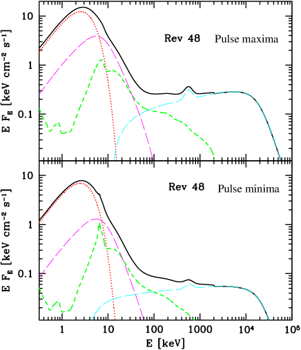
Figure 10: Spectral components of the fits to the pulse maxima (upper panel) and minima (lower panel). The dotted and long-dashed curves show the unscattered blackbody, and Compton scattering from thermal (red) and non-thermal electrons (cyan), including a component from $e^{\pm}$ pair annihilation, important around 511 keV. The short-dashed (green) curve shows the component from Compton reflection, including the Fe K${\alpha}$ line.

We see, however, that there is significant softening of the Comptonized part of the spectrum during pulse minima. This is reflected in the ratio, $\ell_{\rm h}/\ell_{\rm s}$, being significantly smaller. The ratio $\ell_{\rm h}/\ell_{\rm s}$, or, equivalently, $L_{\rm h}/L_{\rm s}$, is between the power supplied to the electrons in the Comptonizing plasma and that in soft disc blackbody photons irradiating the plasma. Our fits do not require an additional component in soft photons not irradiating the hot plasma and thus $L_{\rm s}$ corresponds to the luminosity in the entire disc blackbody emission.

As implied by the value of the bolometric flux in Table 2 (see also Fig. 9), the value of $L_{\rm s}$ (which dominates the bolometric flux) decreases by a factor of $\simeq 2$ during minima. Given the corresponding decrease of $L_{\rm h}/L_{\rm s}$ by a factor of $\simeq 2$, we find that $L_{\rm h}$ decreased by $\sim 4$. Conversely, there is an increase in the relative power supplied to the electrons in the plasma during pulse maxima by a factor of $\sim$2.

It should be noted that the spectrum from the pulse maxima contains both the end of the rising phase and the beginning of the declining phase of each pulse, and thus it is an average of the harder rising and the softer declining phases.

The other best-fit parameters for the two spectra are consistent with being the same within the measurement uncertainties. Given the importance of $e^{\pm}$ pair production, the contribution to the total optical depth, $\tau$, from the ionization electrons is relatively weakly constrained, especially in the high-flux state, when it is consistent with being null (i.e., with all scattering plasma formed by pair production). The corresponding range of the total optical depth, $\tau$, is much narrower; however, the eqpair model does not allow the uncertainties in $\tau$ to be calculated directly as it is not a free parameter.

6 Summary

We have presented INTEGRAL and RXTE data for GRS 1915$+$105 from INTEGRAL’s Revolution 48 in 2003 March. The source was found to exhibit a novel type of variability which we call $\xi$. The continuous 100 ks observations, due to INTEGRAL’s eccentric orbit, allowed us to classify this new variability that dominated the entire JEM-X 3–35 keV lightcurve, and is characterized by repeated 5-minute pulses. The simultaneous RXTE/PCA observations showed in one pointing a series of nine $\sim 5$ minute pulses, corresponding to the pattern seen by JEM-X. By examining the source behaviour in terms of flux-hardness correlations as well as individual pulse shape, we have shown that the rising phases of the pulses are harder and shorter than the declining phases, contrary to what is observed in the $\rho$ and $\kappa$ classes of Belloni et al. (2000) which this new variability class otherwise resembles. Simple modelling of the fast spectral variability confirms a negative correlation between hardness and flux but shows no obvious correlation between flux and inner disc temperature or radius, suggesting that the pulses are largely isothermal. Loop-like features, traced out by the pulses in the colour-colour diagram are interpreted as limit-cycle oscillations probably due to delayed feedback in the inner accretion disc.

Broadband spectral modelling of co-added spectra for the pulse maxima and minima respectively, using eqpair, showed that the spectra of maxima and minima both belong to spectral state A, according to the classification by Belloni et al. (2000), and were essentially similar, except for a significant softening of the Comptonized part of the spectrum during minima. The similarity of the spectra was also confirmed in the plot of the 2–20 keV against the 20–50 keV PCA fluxes which was essentially linear, both throughout the whole observation and solely during the pulses.

We have also seen that there is essentially no correlation between $T_{\rm in}$ and the flux during the pulses, again supporting the suggestion that they are isothermal. This implies that this new variability pattern in itself is largely isothermal by nature. The fact that the spectra do not change between the pulse maxima and the pulse minima (except for the flux level) and that the pulses are described by a fast rise and a slow decline indicates that the variability is not representative of oscillations between spectral states (as e.g. class $\rho$ in Belloni et al. (2000)). We attributed the variability to limit-cycle oscillations which are probably due to delayed feedback in the inner accretion disc. However, the variability could also result from flares in the accretion disc arising from instabilities in the accretion rate.

Recently, Tagger et al. (2004) have shown, based on the work by Fitzgibbon et al. (priv. comm.), that GRS 1915$+$105 always seems to follow the same pattern of transition through all 12 classes as defined by Belloni et al. (2000). This may suggest that GRS 1915$+$105 simply displays a repeating continuum of all possible configurations and that we caught it in an intermediate class between two previously known ones. This implies that more variability classes remain to be observed and that, with continued monitoring of GRS 1915$+$105, we should be able to observe other classes of variability behaviour and gain a better understanding of this mystifying source.

- (1) Anders, E., & Ebihara, M. 1982, Geochim. Cosmochim. Acta, 46, 2363
- (2) Arnaud, K. A. 1996, in Jacoby G. H., Barnes J., eds., Astronomical Data Analysis Software and Systems V, ASP Conf. Series Vol. 101, San Francisco, p. 17
- Belloni et al. (1997) Belloni, T., Méndez, M., King, A.R., van der Klis, M., & van Paradijs, J. 1997, ApJ, 488, L109
- Belloni et al. (2000) Belloni, T., Klein-Wolt, M., Méndez, M., van der Klis, M., & van Paradijs, J. 2000, A&A, 355, 271
- (5) Beloborodov, A.M. 1999, in ASP Conf. Ser. 161, High Energy Processes in Accreting Black Holes, ed. J. Poutanen & R. Svensson (San Francisco: ASP), 295
- Cadolle-Bel et al. (2004) Cadolle-Bel, M., Rodriguez, J., Sizun, P., et al. 2004, A&A, 426, 659
- Castro-Tirado et al. (1992) Castro-Tirado, A.J., Brandt, S., & Lund, N. 1992, IAUC 5590
- Chapuis & Corbel (2004) Chapuis, C., & Corbel, S. 2004, A&A, 414, 659
- (9) Coppi, P.S. 1992, MNRAS, 258, 657
- (10) Coppi, P.S. 1999, in ASP Conf. Ser. Vol. 161, High Energy Processes in Accreting Black Holes, ed. J. Poutanen & R. Svensson (San Francisco: ASP), 375
- Courvoisier et al. (2003) Courvoisier, T. J. L., Walter, R., Beckmann, V., et al. 2003, A&A, 411, L53
- Dhawan et al. (2000) Dhawan, V., Mirabel, I.F., & Rodríguez, L.F. 2000, ApJ, 543, 373
- Dickey & Lockman (1990) Dickey, J.M., & Lockman, F.J. 1990, ARA&A, 28, 215
- (14) Done, C., Mulchaey, J. S., Mushotzky, R. F., & Arnaud, K. A. 1992, ApJ, 395, 275
- Fender et al. (1999) Fender, R.P., Garrington, S.T., McKay, D.J., et al. 1999, MNRAS, 304, 865
- Fender & Belloni (2004) Fender, R., & Belloni, T. 2004, ARA&A, 42, 317
- Fuchs et al. (2003) Fuchs, Y., Rodriguez, J., Mirabel, I.F., et al. 2003, A&A, 409, L35
- (18) Gierliński, M., Zdziarski, A.A., Poutanen, J., et al. 1999, MNRAS, 309, 496
- Greiner et al. (2001) Greiner, J., Cuby, J.G., McCaughrean, M.J., Castro-Tirado, A., & Mennickent, R.E. 2001, A&A, 373, L37
- Hannikainen et al. (2003) Hannikainen, D.C., Vilhu, O., Rodriguez, J., et al. 2003, A&A, 411, L415
- Harlaftis & Greiner (2004) Harlaftis, E., & Greiner, J. 2004, A&A, 414, L13
- Knodlseder et al. (2004) Knödlseder, J., et al. 2004, Proceedings of the 5th INTEGRAL Workshop, Munich, Feb 16–20, 2004, ESA-SP 552.
- Lebrun et al. (2003) Lebrun, F., Leroy, J.P., Lavocat, P., et al. 2003, A&A, 411, L141
- Lund et al. (2003) Lund, N., Budtz-Jørgensen, C., Westergaard, N.J., et al. 2003, A&A, 411, L231
- (25) Magdziarz, P., & Zdziarski, A.A. 1995, MNRAS, 273, 837
- Mas-Hesse et al. (2003) Mas-Hesse, J.M., A. Giménez, J.L. Culhane, et al. 2003, A&A, 411, L261
- Merloni et al. (2000) Merloni, A., Fabian, A.C., & Ross, R.R. 2000, MNRAS, 313, 193
- Mitsuda et al. (1984) Mitsuda, K., Inoue, H., Koyama, K., et al. 1984, PASJ, 36, 741
- Miyamoto et al. (2003) Miyamoto, S., Kitamoto, S., Hayashida, K., & Egoshi, W., 1995, ApJ, 442, L13
- Morgan et al. (1997) Morgan, E.H., Remillard, R.A., & Greiner, J. 1997, ApJ, 482, 993
- Poutanen & Coppi (1998) Poutanen, J., & Coppi, P. 1998, Physica Scripta, T77, 57
- Poutanen & Svensson (1996) Poutanen, J., & Svensson, R. 1996, ApJ, 470, 249
- Poutanen et al. (1997) Poutanen, J., Krolik, J.H., & Ryde, F. 1997, MNRAS, 292, L21
- Rodriguez et al. (2002) Rodriguez, J., Varnière, P., Tagger, M., & Durouchoux, P. 2002, A&A, 387, 487
- Rodriguez et al. (2003) Rodriguez, J., Corbel, S., & Tomsick, J.A. 2003, ApJ, 595, 1032
- Rodriguez et al. (2004a) Rodriguez, J., Corbel, S., Hannikainen, D.C., et al. 2004a, ApJ, 615, 416
- Rodriguez et al. (2004b) Rodriguez, J., Cabanac, C., Hannikainen, et al., 2004b, astro-ph/0412555
- (38) Rodríguez, L.F., & Mirabel, I.F. 1999, ApJ, 511, 398
- Shimura & Takahara (1995) Shimura, T., & Takahara, F. 1995, ApJ,445, 780
- Skinner & McConnell (2003) Skinner, G., & McConnell, P. 2003, A&A, 411, L123
- (41) Sobolewska, M.A., & Życki, P. T. 2003, A&A, 400, 553
- Tagger et al. (2004) Tagger, M., Varnière, P., Rodriguez, J., & Pellat, R. 2004, ApJ, 607, 410
- Ubertini et al. (2003) Ubertini, P., Lebrun, F., Di Cocco, G., et al. 2003, A&A, 411, L131
- Vedrenne et al. (2003) Vedrenne, G., Roques, J.P., Schoenfelder, V., et al. 2003, A&A, 411, L63
- Vilhu & Nevalainen (1998) Vilhu, O., & Nevalainen, J. 1998, ApJ, 508, L85
- (46) Vilhu, O., Poutanen, J., Nikula, P., & Nevalainen, J. 2001, ApJ, 553, L51
- vilhu (03) Vilhu, O., Hjalmarsdotter, L., Zdziarski, A.A., et al. 2003, A&A, 411, L405
- Winkler et al. (2003) Winkler, C., Courvoisier, T.J.-L., DiCocco, G., et al. 2003, A&A, 411, L1
- Zdziarski et al. (2001) Zdziarski, A.A., Grove, J.E., Poutanen, J., Rao, A.R., & Vadawale, S.V. 2001, ApJ, 554, L45
- (50) Zdziarski, A.A., Gierliński, M., Mikołajewska, J., et al. 2004, MNRAS, 351, 791