Lensed CMB power spectra from all-sky correlation functions

Abstract

Weak lensing of the CMB changes the unlensed temperature anisotropy and polarization power spectra. Accounting for the lensing effect will be crucial to obtain accurate parameter constraints from sensitive CMB observations. Methods for computing the lensed power spectra using a low-order perturbative expansion are not good enough for percent-level accuracy. Non-perturbative flat-sky methods are more accurate, but curvature effects change the spectra at the $0.3$–$1\%$ level. We describe a new, accurate and fast, full-sky correlation-function method for computing the lensing effect on CMB power spectra to better than $0.1\%$ at $l\lesssim 2500$ (within the approximation that the lensing potential is linear and Gaussian). We also discuss the effect of non-linear evolution of the gravitational potential on the lensed power spectra. Our fast numerical code is publicly available.

I Introduction

The CMB temperature and polarization anisotropies are being measured with ever increasing precision. The statistics of the anisotropies already provide valuable limits on cosmological parameters, as well as constraints on early-universe physics. As we enter the era of precision measurement, with signal-dominated observations out to small angular scales, non-linear effects will become increasingly important. One of the most significant of these over scales of most interest for parameter estimation is weak gravitational lensing by large scale structure. Fortunately it can be modelled accurately as a second-order effect: the linear gravitational potential along the line of sight lenses the linear perturbations at the last scattering surface (see e.g. Refs. Seljak (1996); Zaldarriaga and Seljak (1998a); Hu (2000a) and references therein). Modelling of fully non-linear evolution is not required for the near future on scales of several arcminutes (corresponding to multipoles $l\lesssim 2000$) for the temperature and electric polarization power spectra. Non-linear corrections can easily be applied to the lensing potential if and when required, provided that its non-Gaussianity can be ignored Seljak (1996).

In principle, the weak-lensing contribution to the observed sky can probably be subtracted given sufficiently accurate and clean high-resolution observations. Early work in this area Seljak and Zaldarriaga (1999); Guzik et al. (2000); Hu (2001); Hu and Okamoto (2002) suggested a limit on the accuracy of this reconstruction due to the statistical nature of the (unknown) unlensed CMB fields. More recently, it has been argued that polarization removes this limit in models where lensing is the only source of $B$-mode polarization on small scales Hirata and Seljak (2003). If subtraction could be done exactly we could recover the unlensed Gaussian sky, and use this for all further analysis. However current methods for subtracting the lensing contribution are approximate, and not easy to apply to realistic survey geometries. The result of imperfect lensing subtraction is a sky with complicated, non-Gaussian statistics of the signal, and significantly more complicated noise properties than the original (lensed) observations. For observations in the near future, a much simpler method to account for the lensing effect is to work with the lensed sky itself, modelling the lensing effect by the expected change in the power spectra and their covariances. The effects of lensing non-Gaussianities on the covariance of the temperature and $E$-mode polarization power spectra are likely to be small, but this will not be the case for the $B$-mode spectrum once thermal-noise levels permit imaging of the lens-induced $B$ modes Smith et al. (2004). In this paper we discuss how to compute the lensed power spectra accurately. The simulation of lensed skies and the effect on parameter estimation is discussed in Ref. Lewis (2005).

On scales where the non-Gaussianity of the lensing potential can be ignored, the calculation of the lensed power spectra is straightforward in principle. However, achieving good accuracy on both large and small scales for all the CMB observables is surprisingly difficult. The lensing action on the CMB fields at scales approaching the r.m.s. of the lensing deflection angle ($\sim 3\,\mathrm{arcmin}$) cannot be accurately described with a first-order Taylor expansion, as in the full-sky harmonic method of Ref. Hu (2000a). There is not much power in the unlensed CMB on such scales, but a first-order Taylor expansion still gives lensed power spectra that are inaccurate at the percent level for $l\gtrsim 1000$. The lensed CMB on scales well below the diffusion scale is generated by the action of small-scale weak lenses on the (relatively) large-scale unlensed CMB, and a Taylor expansion should become more accurate again Seljak and Zaldarriaga (2000). (However, non-linear effects are also important on such scales.) The breakdown of the Taylor expansion can be easily fixed by using the flat-sky correlation-function methods of Refs. Seljak (1996); Zaldarriaga and Seljak (1998a), which can handle the dominant effect of the lensing displacement in a non-perturbative manner. However, a new problem then arises on scales where the flat-sky approximation is not valid. As noted in Ref. Hu (2000a), this is not confined to large scales due to the mode-coupling nature of lensing: degree-scale lenses contribute significantly to the lensed power over a wide range of observed scales. In this paper we develop a new method for computing the lensed power spectra that is accurate on all scales where non-Gaussianity due to non-linear effects is not important. We do this by calculating the lensed correlation functions on the spherical sky. This allows us to include both the non-perturbative effects of displacing small-scale CMB fluctuations, and the effects of sky curvature.

This paper is arranged as follows. We start in Section II with a brief introduction to CMB lensing, then in Section III we review previous work on flat-sky correlation-function methods and present our new full-sky method and results. In Section IV we compare our new results with the flat-sky correlation-function results of Refs. Seljak (1996); Zaldarriaga and Seljak (1998a) and the perturbative harmonic result of Ref. Hu (2000a), and explain why the latter is not accurate enough for precision cosmology. The effect of non-linear evolution of the density field on the lensed power spectra is considered in Section V. We end with conclusions, and include some technical results in the appendices.

II CMB lensing

Gradients in the gravitational potential transverse to the line of sight to the last scattering surface cause deviations in the photon propagation, so that points in a direction $\hat{\mathbf{n}}$ actually come from points on the last scattering surface in a displaced direction $\hat{\mathbf{n}}^{\prime}$. Denote the lensed CMB temperature by $\tilde{\Theta}(\hat{\mathbf{n}})$ and the unlensed temperature by $\Theta(\hat{\mathbf{n}})$, so the lensed field is given by $\tilde{\Theta}(\hat{\mathbf{n}})=\Theta(\hat{\mathbf{n}}^{\prime})$. The change in direction on the sky can be described by a displacement vector field $\bm{\alpha}(\hat{\mathbf{n}})\equiv\bm{\nabla}\psi$, so that (symbolically) $\hat{\mathbf{n}}^{\prime}=\hat{\mathbf{n}}+\bm{\nabla}\psi$. Here $\psi$ is the lensing potential which encapsulates the deviations caused by potentials along the line of sight. More rigorously, on a unit sphere the point $\hat{\mathbf{n}}^{\prime}$ is obtained from $\hat{\mathbf{n}}$ by moving a distance $|\bm{\nabla}\psi|$ along a geodesic in the direction of $\bm{\nabla}\psi(\hat{\mathbf{n}})$, where $\bm{\nabla}$ is the covariant derivative on the sphere Challinor and Chon (2002). We assume that the lensing is weak, so that the potentials may be evaluated along the unperturbed path (i.e. we use the Born approximation). Lensing deflections are a few arcminutes, but are coherent over degree scales, so this is a good approximation.

In terms of the zero-shear acceleration potential $\Psi$, the lensing potential in a flat universe with recombination at conformal distance $\chi_{*}$ is given by the line-of-sight integral

$$\psi(\hat{\mathbf{n}})=-2\int_{0}^{\chi_{*}}{\text{d}}\chi\,\Psi(\chi\hat{\mathbf{n}};\eta_{0}-\chi)\frac{\chi_{*}-\chi}{\chi\chi_{*}}.$$ (1)

Here we neglect the very small effect of late-time sources, including reionization, and approximate recombination as instantaneous so that the CMB is described by a single source plane at $\chi=\chi_{*}$. The quantity $\eta_{0}-\chi$ is the conformal time at which the photon was at position $\chi\hat{\mathbf{n}}$. With the Fourier convention

$$\Psi(\mathbf{x};\eta)=\int\frac{{\text{d}}^{3}{\mathbf{k}}}{(2\pi)^{3/2}}\,\Psi({\mathbf{k}};\eta)e^{i{\mathbf{k}}\cdot\mathbf{x}},$$ (2)

and power spectrum

$$\langle\Psi({\mathbf{k}};\eta)\Psi^{*}({\mathbf{k}}^{\prime};\eta^{\prime})\rangle=\frac{2\pi^{2}}{k^{3}}\mathcal{P}_{\Psi}(k;\eta,\eta^{\prime})\delta({\mathbf{k}}-{\mathbf{k}}^{\prime}),$$ (3)

the angular power spectrum of the lensing potential $\psi$ evaluates to

$$C_{l}^{\psi}=16\pi\int\frac{{\text{d}}k}{k}\,\int_{0}^{\chi_{*}}{\text{d}}\chi\,\int_{0}^{\chi_{*}}{\text{d}}\chi^{\prime}\,\mathcal{P}_{\Psi}(k;\eta_{0}-\chi,\eta_{0}-\chi^{\prime})j_{l}(k\chi)j_{l}(k\chi^{\prime})\left(\frac{\chi_{*}-\chi}{\chi_{*}\chi}\right)\left(\frac{\chi_{*}-\chi^{\prime}}{\chi_{*}\chi^{\prime}}\right).$$ (4)

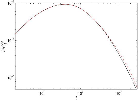
Figure 1: The power spectrum of the lensing potential for a concordance $\Lambda$CDM model. The linear theory spectrum (solid) is compared with the same model including non-linear corrections (dashed) from halofit Smith et al. (2003) using Eq. (67).

In linear theory we can define a transfer function $T_{\Psi}(k,\eta)$ so that $\Psi({\mathbf{k}};\eta)=T_{\Psi}(k,\eta)\mathcal{R}({\mathbf{k}})$ where $\mathcal{R}({\mathbf{k}})$ is the primordial comoving curvature perturbation (or other variable for isocurvature modes). We then have

$$C_{l}^{\psi}=16\pi\int\frac{{\text{d}}k}{k}\,\mathcal{P}_{\mathcal{R}}(k)\left[\int_{0}^{\chi_{*}}{\text{d}}\chi\,T_{\Psi}(k;\eta_{0}-\chi)j_{l}(k\chi)\left(\frac{\chi_{*}-\chi}{\chi_{*}\chi}\right)\right]^{2}$$ (5)

where the primordial power spectrum is $\mathcal{P}_{\mathcal{R}}(k)$. This can be computed easily numerically using camb Lewis et al. (2000), and a typical spectrum is shown in Fig. 1.

III Lensed correlation function

III.1 Flat-sky limit

We start by calculating the lensed correlation function in the flat-sky limit, broadly following the method of Ref. Seljak (1996). We use a 2D Fourier transform of the temperature field

$$\Theta(\mathbf{x})=\int\frac{{\text{d}}^{2}{\mathbf{l}}}{2\pi}\,\Theta({\mathbf{l}})e^{i{\mathbf{l}}\cdot\mathbf{x}},$$ (6)

and the power spectrum for a statistically isotropic field is then

$$\langle\Theta({\mathbf{l}})\Theta^{*}({\mathbf{l}}^{\prime})\rangle=C_{l}^{\Theta}\delta({\mathbf{l}}-{\mathbf{l}}^{\prime}).$$ (7)

Lensing re-maps the temperature according to

$$\tilde{\Theta}(\mathbf{x})=\Theta(\mathbf{x}+\bm{\alpha}),$$ (8)

where in linear theory the displacement vector $\bm{\alpha}$ is a Gaussian field. We shall require its correlation tensor $\langle\alpha_{i}(\mathbf{x})\alpha_{j}(\mathbf{x}^{\prime})\rangle$ to compute the lensed CMB power spectrum. Introducing the Fourier transform of the lensing potential, $\psi({\mathbf{l}})$, we have

$$\bm{\alpha}(\mathbf{x})=i\int\frac{{\text{d}}^{2}{\mathbf{l}}}{2\pi}\,{\mathbf{l}}\psi({\mathbf{l}})e^{i{\mathbf{l}}\cdot\mathbf{x}},$$ (9)

so that

$$\langle\alpha_{i}(\mathbf{x})\alpha_{j}(\mathbf{x}^{\prime})\rangle=\int\frac{{\text{d}}^{2}{\mathbf{l}}}{(2\pi)^{2}}l_{i}l_{j}C_{l}^{\psi}e^{i{\mathbf{l}}\cdot(\mathbf{x}-\mathbf{x}^{\prime})}.$$ (10)

By symmetry, the correlator can only depend on $\delta_{ij}$ and the trace-free tensor $r_{\langle i}r_{j\rangle}$, where ${\mathbf{r}}\equiv\mathbf{x}-\mathbf{x}^{\prime}$. Evaluating the coefficients of these two terms by taking the trace of the correlator, and its contraction with $r^{i}r^{j}$, we find

$$\langle\alpha_{i}(\mathbf{x})\alpha_{j}(\mathbf{x}^{\prime})\rangle=\frac{1}{4\pi}\int{\text{d}}l\,l^{3}C_{l}^{\psi}J_{0}(lr)\delta_{ij}-\frac{1}{2\pi}\int{\text{d}}l\,l^{3}C_{l}^{\psi}J_{2}(lr)\hat{r}_{\langle i}\hat{r}_{j\rangle},$$ (11)

where $J_{n}(x)$ is a Bessel function of order $n$. Note that the trace-free term is analytic at $r=0$ due to the small-$r$ behaviour of $J_{2}(lr)$. Following Ref. Seljak (1996), let us denote $\langle\bm{\alpha}(\mathbf{x})\cdot\bm{\alpha}(\mathbf{x}^{\prime})\rangle$ by $C_{\text{gl}}(r)$ so that

$$C_{\text{gl}}(r)=\frac{1}{2\pi}\int{\text{d}}l\,l^{3}C_{l}^{\psi}J_{0}(lr).$$ (12)

Similarly we define the anisotropic coefficient

$$C_{\text{gl},2}(r)=\frac{1}{2\pi}\int{\text{d}}l\,l^{3}C_{l}^{\psi}J_{2}(lr),$$ (13)

so that

$$\langle\alpha_{i}(\mathbf{x})\alpha_{j}(\mathbf{x}^{\prime})\rangle=\frac{1}{2}C_{\text{gl}}(r)\delta_{ij}-C_{\text{gl},2}(r)\hat{r}_{\langle i}\hat{r}_{j\rangle}.$$ (14)

The lensed correlation function $\tilde{\xi}(r)$ is given by

$$\tilde{\xi}(r) \equiv \langle\tilde{\Theta}(\mathbf{x})\tilde{\Theta}(\mathbf{x}^{\prime})\rangle$$ (15)

$$= \int\frac{{\text{d}}^{2}{\mathbf{l}}}{(2\pi)^{2}}C_{l}^{\Theta}e^{i{\mathbf{l}}\cdot{\mathbf{r}}}\langle e^{i{\mathbf{l}}\cdot[\bm{\alpha}(\mathbf{x})-\bm{\alpha}(\mathbf{x}^{\prime})]}\rangle,$$

where we have assumed that the CMB and lensing potential are independent (i.e. we are neglecting the large scale correlation that arises from the integrated-Sachs-Wolfe effect and has only a tiny effect on the lensed CMB). Since we are assuming $\bm{\alpha}$ is a Gaussian field, ${\mathbf{l}}\cdot[\bm{\alpha}(\mathbf{x})-\bm{\alpha}(\mathbf{x}^{\prime})]$ is a Gaussian variate and the expectation value in Eq. (15) reduces to

$$\langle e^{i{\mathbf{l}}\cdot[\bm{\alpha}(\mathbf{x})-\bm{\alpha}(\mathbf{x}^{\prime})]}\rangle = \exp\left(-\frac{1}{2}\langle[{\mathbf{l}}\cdot(\bm{\alpha}-\bm{\alpha}^{\prime})]^{2}\rangle\right)$$ (16)

$$= \exp\left(-\frac{1}{2}l^{2}[\sigma^{2}(r)+\cos 2(\phi_{\mathbf{l}}-\phi_{\mathbf{r}})C_{\text{gl},2}(r)]\right),$$

where we have used $l^{i}l^{j}\hat{r}_{\langle i}\hat{r}_{j\rangle}=l^{2}\cos 2(\phi_{\mathbf{l}}-\phi_{\mathbf{r}})/2$ and defined $\sigma^{2}(r)\equiv C_{\text{gl}}(0)-C_{\text{gl}}(r)$. Here, e.g. $\phi_{\mathbf{l}}$ is the angle between ${\mathbf{l}}$ and the $x$-axis. The $\cos 2(\phi_{\mathbf{l}}-\phi_{\mathbf{r}})$ term in Eq. (16) is difficult to handle analytically. Instead, we expand the exponential and integrate term by term. Expanding to second order in $C_{\text{gl},2}$, we find

$$\tilde{\xi}(r) = \frac{1}{2\pi}\int l{\text{d}}l\,C_{l}e^{-l^{2}\sigma^{2}(r)/2}\left[\left(1+\frac{1}{16}l^{4}C_{\text{gl},2}^{2}(r)\right)J_{0}(lr)+\frac{1}{2}l^{2}C_{\text{gl},2}(r)J_{2}(lr)+\frac{1}{16}l^{4}C_{\text{gl},2}^{2}(r)J_{4}(lr)\right].$$ (17)

Expanding to this order is sufficient to get the lensed power spectrum to second order in $C_{l}^{\psi}$; higher order terms in $C_{\text{gl},2}$ only contribute at the $O(10^{-4})$ level on the scales of interest. Note that the $\exp(-l^{2}\sigma^{2}/2)$ term is easily handled without resorting to a perturbative expansion in $C_{l}^{\psi}$. Since $\sigma^{2}$ is significantly less than $C_{\text{gl},2}$ (as shown in Fig. 2), the perturbative expansion in $C_{\text{gl},2}$ converges much faster than one in $\sigma^{2}$. Equation (17) extends the result of Ref. Seljak (1996) to second order in $C_{\text{gl},2}$.

Figure 2: The functions $\sigma^{2}(\beta)\equiv C_{\text{gl}}(0)-C_{\text{gl}}(\beta)$ [solid] and $C_{\text{gl},2}(\beta)$ [dashed] as a function of angular separation $\beta$ (in radians) for a typical concordance model. The results are calculated using the full-sky definitions of Eqs. (35), and use the linear power spectrum for $C_{l}^{\psi}$.

III.1.1 Polarization

The polarization calculation is also straightforward in the flat-sky limit Zaldarriaga and Seljak (1998b). We use the spin $-2$ polarization $P\equiv Q+iU$, where $Q$ and $U$ are the Stokes’ parameters measured with respect to the fixed basis composed of the $x$ and $-y$ axes. Expanding $P(\mathbf{x})$ in terms of the Fourier transforms of its electric ($E$) and magnetic ($B$) parts, we have

$$P(\mathbf{x})=-\int\frac{{\text{d}}^{2}{\mathbf{l}}}{2\pi}\,(E({\mathbf{l}})-iB({\mathbf{l}}))e^{-2i\phi_{{\mathbf{l}}}}e^{i{\mathbf{l}}\cdot\mathbf{x}},$$ (18)

where $(\partial_{x}-i\partial_{y})^{2}e^{i{\mathbf{l}}\cdot\mathbf{x}}/l^{2}=-e^{-2i\phi_{{\mathbf{l}}}}e^{i{\mathbf{l}}\cdot\mathbf{x}}$ is a spin -2 flat-sky harmonic. The polarization correlation functions are defined as

$$\xi_{+}(r) \equiv \langle e^{-2i\phi_{\mathbf{r}}}P^{*}(\mathbf{x})e^{2i\phi_{\mathbf{r}}}P(\mathbf{x}^{\prime})\rangle,$$ (19)

$$\xi_{-}(r) \equiv \langle e^{2i\phi_{\mathbf{r}}}P(\mathbf{x})e^{2i\phi_{\mathbf{r}}}P(\mathbf{x}^{\prime})\rangle,$$ (20)

$$\xi_{X}(r) \equiv \langle\Theta(\mathbf{x})e^{2i\phi_{\mathbf{r}}}P(\mathbf{x}^{\prime})\rangle,$$ (21)

where $\pi-\phi_{\mathbf{r}}$ is the angle to rotate the $x$-axis onto the vector joining $\mathbf{x}$ and $\mathbf{x}^{\prime}$, so that e.g. $e^{2i\phi_{\mathbf{r}}}P(\mathbf{x})$ is the polarization on the basis adapted to $\mathbf{x}$ and $\mathbf{x}^{\prime}$. Then the lensed correlation functions to second-order in $C_{\text{gl},2}$ are

$$\tilde{\xi}_{+}(r) = \frac{1}{2\pi}\int l{\text{d}}l\,(C_{l}^{E}+C_{l}^{B})e^{-l^{2}\sigma^{2}(r)/2}\left[\left(1+\frac{1}{16}l^{4}C_{\text{gl},2}^{2}(r)\right)J_{0}(lr)\right.$$ (22)

$$\phantom{\frac{1}{2\pi}\int l{\text{d}}l\,(C_{l}^{E}+C_{l}^{B})e^{-l^{2}\sigma^{2}(r)/2}+}\left.+\frac{1}{2}l^{2}C_{\text{gl},2}(r)J_{2}(lr)+\frac{1}{16}l^{4}C_{\text{gl},2}^{2}(r)J_{4}(lr)\right],$$

$$\tilde{\xi}_{-}(r) = \frac{1}{2\pi}\int l{\text{d}}l\,(C_{l}^{E}-C_{l}^{B})e^{-l^{2}\sigma^{2}(r)/2}\left[\left(1+\frac{1}{16}l^{4}C_{\text{gl},2}^{2}(r)\right)J_{4}(lr)\right.$$ (23)

$$\phantom{\frac{1}{2\pi}\int l{\text{d}}l\,(C_{l}^{E}-C_{l}^{B})e^{-l^{2}\sigma^{2}(r)/2}+}\left.+\frac{1}{2}l^{2}C_{\text{gl},2}(r)\frac{1}{2}[J_{2}(lr)+J_{6}(lr)]+\frac{1}{16}l^{4}C_{\text{gl},2}^{2}(r)\frac{1}{2}[J_{0}(lr)+J_{8}(lr)]\right],$$

$$\tilde{\xi}_{X}(r) = \frac{1}{2\pi}\int l{\text{d}}l\,C_{l}^{X}e^{-l^{2}\sigma^{2}(r)/2}\left[\left(1+\frac{1}{16}l^{4}C_{\text{gl},2}^{2}(r)\right)J_{2}(lr)+\frac{1}{2}l^{2}C_{\text{gl},2}(r)\frac{1}{2}[J_{0}(lr)+J_{4}(lr)]\right.$$ (24)

$$\phantom{\frac{1}{2\pi}\int l{\text{d}}l\,C_{l}^{X}e^{-l^{2}\sigma^{2}(r)/2}+}\left.+\frac{1}{16}l^{4}C_{\text{gl},2}^{2}(r)\frac{1}{2}[J_{2}(lr)+J_{6}(lr)]\right].$$

Here $C_{l}^{E}$ and $C_{l}^{B}$ are the $E$-mode and $B$-mode power spectra, and $C_{l}^{X}$ is the $\Theta$-$E$ cross-correlation. This is the straightforward extension of the result in Ref. Zaldarriaga and Seljak (1998b) to higher order; see that paper for further details of the calculation.

The lensed $\tilde{\xi}_{+}(r)$ has the same structure as for the temperature since the unlensed correlation functions involve the same $J_{0}(lr)$, and there are no complications due to the different local bases defined by the displacement ${\mathbf{r}}$ and its image under lensing ${\mathbf{r}}-\bm{\alpha}^{\prime}+\bm{\alpha}$ since the phase factors from the rotations cancel. This is not the case for the lensed $\tilde{\xi}_{-}(r)$ and $\tilde{\xi}_{X}(r)$.

III.1.2 Limber approximation

At high $l$ the power spectrum $\mathcal{P}_{\Psi}(k)$ varies slowly compared to the spherical Bessel functions in Eq. (4), which pick out the scale $k\sim l/\chi$. Using

$$\int k^{2}{\text{d}}k\,j_{l}(k\chi)j_{l}(k\chi^{\prime})=\frac{\pi}{2\chi^{2}}\delta(\chi-\chi^{\prime}),$$ (25)

we can Limber-approximate $C_{l}^{\psi}$ as

$$C_{l}^{\psi}\approx\frac{8\pi^{2}}{l^{3}}\int_{0}^{\chi_{*}}\chi{\text{d}}\chi\,\mathcal{P}_{\Psi}(l/\chi;\eta_{0}-\chi)\left(\frac{\chi_{*}-\chi}{\chi_{*}\chi}\right)^{2}.$$ (26)

Changing variables to $k=l/\chi$, we find

$$C_{\text{gl}}(r)\approx 4\pi\int{\text{d}}k\,\int{\text{d}}\chi\mathcal{P}_{\Psi}(k;\eta_{0}-\chi)\left(\frac{\chi_{*}-\chi}{\chi_{*}}\right)^{2}J_{0}(k\chi r),$$ (27)

in agreement with Ref. Seljak (1996) if we note that his $P_{\phi}(k)=\mathcal{P}_{\Psi}(k)/(4\pi k^{3})$ outside radiation-domination. Ref. Seljak (1996) also defines $C_{\text{gl},2}(r)$ as (in our notation)

$$C_{\text{gl},2}(r)\approx 4\pi\int{\text{d}}k\,\int{\text{d}}\chi\mathcal{P}_{\Psi}(k;\eta_{0}-\chi)\left(\frac{\chi_{*}-\chi}{\chi_{*}}\right)^{2}J_{2}(k\chi r),$$ (28)

which is the Limber-approximation version of Eq. (13). For the results of this paper we do not use the Limber approximation, though the approximation is rather good.

III.2 Spherical sky

The flat-sky result for the lensed correlation function is non-perturbative in $\sigma^{2}(r)$ and this turns out to be crucial for getting high accuracy in the lensed power spectrum on arcminute scales. Consider the contribution to the lensed correlation functions from the unlensed CMB at multipole $l$. Both $\sigma^{2}$ and $C_{\text{gl},2}$ appear with a factor $l^{2}$ and so the (dominant) $l^{2}\sigma^{2}$ term cannot be handled accurately with a low-order expansion at high $l$. Physically, this is because the typical lensing displacement is then comparable to the wavelength of the unlensed fluctuation, and so approximating the fluctuation as a gradient over the scale of the lensing displacement is inaccurate. The error from this gradient approximation on the lensed power spectra will be large on any scale $|{\mathbf{l}}|$ where the dominant contribution is from unlensed fluctuations with wavenumber ${\mathbf{l}}^{\prime}$ comparable to the typical lensing displacement at scale $|{\mathbf{l}}-{\mathbf{l}}^{\prime}|$.

As noted in the Introduction, the small-scale cut-off in the power in the unlensed fluctuations due to diffusion damping means that the gradient approximation should not get uniformly worse on small scales; the approximation should be poorest on scales of a few arcminutes. We also noted that the the flat-sky approximation will be suspect on large scales, and also on any scale where the dominant contribution is from large-scale lenses, i.e.  those for which their mode-coupled wavenumber $|{\mathbf{l}}-{\mathbf{l}}^{\prime}|$ small. What is needed for an accurate calculation (on all scales where non-linearities in the lensing potential are not important), is a non-perturbative treatment of $\sigma^{2}$ and a proper treatment of curvature effects in the correlation functions. In this section we show how to generalize the flat-sky calculation to spherical correlation functions.

On the full sky we can expand the temperature field in spherical harmonics

$$\Theta(\hat{\mathbf{n}})=\sum_{lm}\Theta_{lm}Y_{lm}(\hat{\mathbf{n}}),$$ (29)

and the temperature correlation function is defined by

$$\xi(\beta)\equiv\langle\Theta(\hat{\mathbf{n}}_{1})\Theta(\hat{\mathbf{n}}_{2})\rangle,$$ (30)

where $\beta$ is the angle between the two directions ($\hat{\mathbf{n}}_{1}\cdot\hat{\mathbf{n}}_{2}=\cos\beta$). The power spectrum is defined as the variance of the harmonic coefficients $C_{l}^{\Theta}\equiv\langle|\Theta_{lm}|^{2}\rangle$ for a statistically-isotropic ensemble.

Figure 3: The geometry of the weak lensing deflections (shown without curvature for clarity).

We define a spin-1 deflection field ${}_{1}\alpha\equiv\bm{\alpha}\cdot(\mathbf{e}_{\theta}+i\mathbf{e}_{\phi})$, where $\mathbf{e}_{\theta}$ and $\mathbf{e}_{\phi}$ are the unit basis vectors of a spherical-polar coordinate system. Rotating to the basis defined by the geodesic connecting $\hat{\mathbf{n}}_{1}$ and $\hat{\mathbf{n}}_{2}$, the spin-1 deflection (denoted with an overbar in the geodesic basis) has real and imaginary components

$$\alpha_{1}\cos\psi_{1}=\Re{}_{1}\bar{\alpha}(\hat{\mathbf{n}}_{1}),\quad\alpha_{1}\sin\psi_{1}=\Im{}_{1}\bar{\alpha}(\hat{\mathbf{n}}_{1}),\quad$$ (31)

and similarly at $\hat{\mathbf{n}}_{2}$. Here, $\alpha_{1}=|\bm{\alpha}(\hat{\mathbf{n}}_{1})|$ is the length of the lensing displacement at $\hat{\mathbf{n}}_{1}$ and $\psi_{1}$ is the angle it makes with the geodesic from $\hat{\mathbf{n}}_{1}$ to $\hat{\mathbf{n}}_{2}$ (see Fig. 3). In terms of these angles we have the lensed correlation function

$$\tilde{\xi}(\beta) = \langle\Theta(\hat{\mathbf{n}}_{1}^{\prime})\Theta(\hat{\mathbf{n}}_{2}^{\prime})\rangle$$ (32)

$$= \sum_{lm}C_{l}^{\Theta}\langle Y_{lm}(\hat{\mathbf{n}}_{1}^{\prime})Y^{*}_{lm}(\hat{\mathbf{n}}_{2}^{\prime})\rangle$$ (33)

$$= \sum_{lmm^{\prime}}C_{l}^{\Theta}d^{l}_{mm^{\prime}}(\beta)\langle Y_{lm}(\alpha_{1},\psi_{1})Y^{*}_{lm^{\prime}}(\alpha_{2},\psi_{2})\rangle.$$ (34)

The easiest way to see the last step is to put $\hat{\mathbf{n}}_{1}$ along the $z$-axis, and $\hat{\mathbf{n}}_{2}$ in the $x$-$z$ plane so that $\hat{\mathbf{n}}_{1}^{\prime}$ has polar coordinates $(\alpha_{1},\psi_{1})$. The harmonic at the deflected position $\hat{\mathbf{n}}_{2}^{\prime}$ can be evaluated by rotation: $Y_{lm}(\hat{\mathbf{n}}_{2}^{\prime})=[\hat{D}^{-1}(0,\beta,0)Y_{lm}](\alpha_{2},\psi_{2})$, where $[\hat{D}Y_{lm}](\hat{\mathbf{n}})$ is a spherical harmonic rotated by the indicated Euler angles. We have neglected the small correlation between the deflection angle and the temperature so that they may be treated as independent fields. The remaining average is over possible realizations of the lensing field.

We assume the lensing potential is Gaussian, so the covariance of the spin-1 deflection field can be determined using the results

$$\langle{}_{1}\bar{\alpha}(\hat{\mathbf{n}}_{1}){}_{1}\bar{\alpha}(\hat{\mathbf{n}}_{2})\rangle = -\sum_{l}\frac{2l+1}{4\pi}l(l+1)C_{l}^{\psi}d^{l}_{-11}(\beta)\equiv-C_{\text{gl},2}(\beta),$$

$$\langle{}_{1}\bar{\alpha}^{*}(\hat{\mathbf{n}}_{1}){}_{1}\bar{\alpha}(\hat{\mathbf{n}}_{2})\rangle = \sum_{l}\frac{2l+1}{4\pi}l(l+1)C_{l}^{\psi}d^{l}_{11}(\beta)\equiv C_{\text{gl}}(\beta).$$ (35)

As in the flat-sky limit, it is convenient to define $\sigma^{2}(\beta)\equiv C_{\text{gl}}(0)-C_{\text{gl}}(\beta)$. The covariance of the Gaussian variates $\Re{}_{1}\bar{\alpha}(\hat{\mathbf{n}}_{1})$, $\Im{}_{1}\bar{\alpha}(\hat{\mathbf{n}}_{1})$, $\Re{}_{1}\bar{\alpha}(\hat{\mathbf{n}}_{2})$ and $\Im{}_{1}\bar{\alpha}(\hat{\mathbf{n}}_{2})$ are determined by Eq. (35). Transforming variables to $\alpha_{1}$, $\psi_{1}$, $\alpha_{2}$ and $\psi_{2}$ we find their probability distribution function

$$\text{Pr}(\alpha_{1},\alpha_{2},\psi_{1},\psi_{2}) = \frac{4\alpha_{1}\alpha_{2}}{(2\pi)^{2}}\frac{e^{-{\textstyle{\frac{1}{2}}}(\alpha_{1}\cos\psi_{1}+\alpha_{2}\cos\psi_{2})^{2}/(\sigma^{2}+2C_{\text{gl}}-C_{\text{gl},2})}}{\sqrt{\sigma^{2}+2C_{\text{gl}}-C_{\text{gl},2}}}$$ (36)

$$\mbox{}\times\frac{e^{-{\textstyle{\frac{1}{2}}}(\alpha_{1}\sin\psi_{1}+\alpha_{2}\sin\psi_{2})^{2}/(\sigma^{2}+2C_{\text{gl}}+C_{\text{gl},2})}}{\sqrt{\sigma^{2}+2C_{\text{gl}}+C_{\text{gl},2}}}\frac{e^{-{\textstyle{\frac{1}{2}}}(\alpha_{1}\cos\psi_{1}-\alpha_{2}\cos\psi_{2})^{2}/(\sigma^{2}+C_{\text{gl},2})}}{\sqrt{\sigma^{2}+C_{\text{gl},2}}}$$

$$\mbox{}\times\frac{e^{-{\textstyle{\frac{1}{2}}}(\alpha_{1}\sin\psi_{1}-\alpha_{2}\sin\psi_{2})^{2}/(\sigma^{2}-C_{\text{gl},2})}}{\sqrt{\sigma^{2}-C_{\text{gl},2}}}.$$

Here and below we have left the dependence of $\sigma^{2}$, $C_{\text{gl}}$ and $C_{\text{gl},2}$ on $\beta$ implicit. Our general strategy to evaluate Eq. (34) is to expand $\text{Pr}(\alpha_{1},\alpha_{2},\psi_{1},\psi_{2})$ in $C_{\text{gl}}$ and $C_{\text{gl},2}$, but not $\sigma^{2}$, before performing the integral over the angles $\psi_{1}$ and $\psi_{2}$ in the expectation value. The remaining integrals over $\alpha_{1}$ and $\alpha_{2}$ then enter through functions of the form

$$X_{imn}\equiv\int_{0}^{\infty}\frac{2\alpha}{\sigma^{2}}\left(\frac{\alpha}{\sigma^{2}}\right)^{i}e^{-\alpha^{2}/\sigma^{2}}d^{l}_{mn}(\alpha)\,{\text{d}}\alpha.$$ (37)

Since terms involving $C_{\text{gl}}(\beta)$ are suppressed at high $l$ (they do not appear in the flat-sky results), while at low $l$ the leading-order result neglecting $C_{\text{gl}}$ and $C_{\text{gl},2}$ altogether is very accurate, we neglect terms involving $C_{\text{gl}}$ entirely. This approximation is very accurate [$<O(10^{-4})$] (for completeness the full second-order result is given in Appendix C). As shown in Fig. 2 the values of $C_{\text{gl},2}$ are much smaller than $\sigma^{2}$, so a perturbative treatment in $C_{\text{gl},2}$ is sufficient as in the flat-sky case. Working to second-order in $C_{\text{gl},2}$, we find

$$\tilde{\xi}\approx\sum_{l}\frac{2l+1}{4\pi}C^{\Theta}_{l}\biggl{\{}X_{000}^{2}d^{l}_{00}+\frac{8}{l(l+1)}C_{\text{gl},2}X_{000}^{\prime\,2}d_{1-1}^{l}+C_{\text{gl},2}^{2}\left(X_{000}^{\prime\,2}d^{l}_{00}+X_{220}^{2}d_{2-2}^{l}\right)\biggr{\}},$$ (38)

where primes denote differentiation with respect to $\sigma^{2}$ [note that the $X_{imn}$ are implicit functions of $\beta$ via the dependence on $\sigma^{2}(\beta)$]. In Appendix B we develop approximations for the integrals $X_{imn}$ which are accurate for all $l$. Applying these approximations, the required $X_{imn}$ are

$$X_{000} \approx e^{-l(l+1)\sigma^{2}/4}$$ (39)

$$X_{220} \approx \frac{1}{4}\sqrt{(l+2)(l-1)l(l+1)}e^{-[l(l+1)-2]\sigma^{2}/4}.$$ (40)

The expansion of these results to $O(\sigma^{2})$ may also be derived straightforwardly by using the series expansion of $d^{l}_{mn}(\alpha)$ for small $\alpha$. (The smallness of $\sigma^{2}$ guarantees that the integral is dominated by the small $\alpha$ region). However, it is important to retain the correct non-perturbative form for high $l$.

In the limit of large $l$ the limiting result $d^{l}_{mn}(\beta)\rightarrow(-1)^{n-m}J_{m-n}(l\beta)$ shows that the full result of Eq. (38) reduces to Eq. (17) in the flat-sky limit and is therefore consistent. In the limit in which the separation angle $\beta\rightarrow 0$ we have

$$\tilde{\xi}(0) = \sum_{l}\frac{2l+1}{4\pi}C^{\Theta}_{l}=\sum_{l}\frac{2l+1}{4\pi}\tilde{C}^{\Theta}_{l},$$ (41)

where $\tilde{C}_{l}^{\Theta}$ is the lensed power spectrum. This expresses the fact that weak lensing does not change the total fluctuation power.

III.2.1 Polarization

We can extend the previous calculation to polarization. Defining Stokes’ parameters with the local $x$-axis along the $\theta$-direction and $y$ along $-\phi$, the quantities $Q\pm iU$ are spin $\mp 2$ respectively. We can expand $Q\pm iU$ in terms of the spin-weight harmonics as Zaldarriaga and Seljak (1997)

$$(Q\pm iU)(\hat{\mathbf{n}})=\sum_{lm}(E_{lm}\mp iB_{lm}){}_{\mp 2}Y_{lm}(\hat{\mathbf{n}}),$$ (42)

which expresses $P\equiv Q+iU$ as the sum of its electric ($E$ or gradient-like) and magnetic ($B$ or curl-like) parts. (Our conventions for the polarization harmonics and correlation functions follow Refs. Lewis et al. (2002); Chon et al. (2004); see these papers for a more thorough introduction). The polarization correlation functions can be defined in terms of the spin $\pm 2$ polarization defined in the physical basis of the geodesic connecting the two positions. As for the temperature, we evaluate the polarization correlation functions by taking $\hat{\mathbf{n}}_{1}$ along the $z$-axis and $\hat{\mathbf{n}}_{2}$ in the $x$-$z$ plane at angle $\beta$ to the $z$-axis. With this geometry, the polar-coordinate basis is already the geodesic basis connecting $\hat{\mathbf{n}}_{1}$ and $\hat{\mathbf{n}}_{2}$ so that the lensed correlation functions are

$$\tilde{\xi}_{+}(\beta) \equiv \langle\tilde{P}^{*}(\hat{\mathbf{n}}_{1})\tilde{P}(\hat{\mathbf{n}}_{2})\rangle,$$ (43)

$$\tilde{\xi}_{-}(\beta) \equiv \langle\tilde{P}(\hat{\mathbf{n}}_{1})\tilde{P}(\hat{\mathbf{n}}_{2})\rangle,$$ (44)

$$\tilde{\xi}_{X}(\beta) \equiv \langle\tilde{\Theta}(\hat{\mathbf{n}}_{1})\tilde{P}(\hat{\mathbf{n}}_{2})\rangle.$$ (45)

Under a lensing deflection the polarization orientation is preserved relative to the direction of the deflection (we are neglecting the small effect of field rotation Hirata and Seljak (2003)), i.e. the polarization undergoes parallel transport. The geometry of the deflections is shown in Fig. 3.

We can easily evaluate the lensed polarization on the connecting geodesic basis (between $\hat{\mathbf{n}}_{1}$ and $\hat{\mathbf{n}}_{2}$) as

$$\tilde{P}(\hat{\mathbf{n}}_{1})=P(\alpha_{1},\psi_{1})e^{-2i\psi_{1}}.$$ (46)

The rotation angle $\psi_{1}$ is that needed to rotate the spin $-2$ polarization from polar coordinates (coinciding with the the $\hat{\mathbf{n}}_{1}$–$\hat{\mathbf{n}}_{1}^{\prime}$ basis at $\hat{\mathbf{n}}_{1}^{\prime}$) to the geodesic basis connecting $\hat{\mathbf{n}}_{1}$ and $\hat{\mathbf{n}}_{2}$.

For the lensed polarization at $\hat{\mathbf{n}}_{2}$ a little more work is required. Let $\chi^{\prime}$ denote the angle between the geodesics connecting $\hat{\mathbf{n}}_{2}$ to $\hat{\mathbf{n}}_{2}^{\prime}$, and $\hat{\mathbf{n}}_{1}$ (along the $z$-axis) to $\hat{\mathbf{n}}_{2}^{\prime}$ (see Fig. 3). The lensed polarization at $\hat{\mathbf{n}}_{2}$ on the geodesic basis adapted to $\hat{\mathbf{n}}_{1}$ and $\hat{\mathbf{n}}_{2}$ is then

$$\tilde{P}(\hat{\mathbf{n}}_{2})=P(\hat{\mathbf{n}}_{2}^{\prime})e^{2i\chi^{\prime}}e^{-2i\psi_{2}}.$$ (47)

We can write $\hat{\mathbf{n}}_{2}^{\prime}$ as the direction obtained by rotating a direction with polar angles $(\alpha_{2},\psi_{2})$ by an angle $\beta$ about the $y$-axis, i.e. $\hat{\mathbf{n}}_{2}^{\prime}=\hat{D}(0,\beta,0)(\alpha_{2},\psi_{2})$. Writing $P$ as $(Q-iU)^{*}$, and using Eq. (42), we have

$$P(\hat{\mathbf{n}})=\sum_{lm}(E_{lm}+iB_{lm})^{*}{}_{+2}Y_{lm}^{*}(\hat{\mathbf{n}}).$$ (48)

Using the rotation properties of the spin-$s$ harmonics (see Appendix A), we then find

$$\tilde{P}(\hat{\mathbf{n}}_{2})=e^{2i\chi^{\prime}}e^{-2i\psi_{2}}e^{-2i\kappa}\sum_{lmm^{\prime}}(E_{lm}+iB_{lm})^{*}D^{l*}_{mm^{\prime}}(0,\beta,0){}_{2}Y_{lm^{\prime}}^{*}(\alpha_{2},\psi_{2}).$$ (49)

The angle $\kappa$ is the rotation about $\hat{\mathbf{n}}_{2}^{\prime}$ that is required to bring the polar basis there onto that obtained by rotating the polar basis at $(\alpha_{2},\psi_{2})$ with $\hat{D}(0,\beta,0)$. Since the latter is aligned with the geodesic basis adapted to $\hat{\mathbf{n}}_{2}$ and $\hat{\mathbf{n}}_{2}^{\prime}$, we have $\kappa=\chi^{\prime}$ and the lensed polarization at $\hat{\mathbf{n}}_{2}$ simplifies to

$$\tilde{P}(\hat{\mathbf{n}}_{2})=e^{-2i\psi_{2}}\sum_{lmm^{\prime}}(E_{lm}+iB_{lm})^{*}d^{l}_{mm^{\prime}}(\beta){}_{2}Y_{lm^{\prime}}^{*}(\alpha_{2},\psi_{2}).$$ (50)

We can now quickly proceed to the following expressions for the lensed polarization correlation functions:

$$\tilde{\xi}_{+}(\beta) = \sum_{lmm^{\prime}}(C_{l}^{E}+C_{l}^{B})d^{l}_{mm^{\prime}}(\beta)\langle e^{2i\psi_{1}}{}_{2}Y_{lm}(\alpha_{1},\psi_{1}){}_{2}Y_{lm^{\prime}}^{*}(\alpha_{2},\psi_{2})e^{-2i\psi_{2}}\rangle,$$ (51)

$$\tilde{\xi}_{-}(\beta) = \sum_{lmm^{\prime}}(C_{l}^{E}-C_{l}^{B})d^{l}_{mm^{\prime}}(\beta)\langle e^{-2i\psi_{1}}{}_{-2}Y_{lm}(\alpha_{1},\psi_{1}){}_{2}Y_{lm^{\prime}}^{*}(\alpha_{2},\psi_{2})e^{-2i\psi_{2}}\rangle,$$ (52)

$$\tilde{\xi}_{X}(\beta) = \sum_{lmm^{\prime}}C_{l}^{X}d^{l}_{mm^{\prime}}(\beta)\langle Y_{lm}(\alpha_{1},\psi_{1}){}_{2}Y_{lm^{\prime}}^{*}(\alpha_{2},\psi_{2})e^{-2i\psi_{2}}\rangle,$$ (53)

where the expectation values are over lensing realizations. Here, $C_{l}^{E}$ and $C_{l}^{B}$ are the power spectra $\langle|E_{lm}|^{2}\rangle$ and $\langle|B_{lm}|^{2}\rangle$ respectively. The cross-correlation power spectrum is $C_{l}^{X}\equiv\langle\Theta_{lm}E_{lm}^{*}\rangle$.

We evaluate the expectation values in Eqs. (51–53) following the earlier calculation for the temperature, i.e. expanding $\text{Pr}(\alpha_{1},\alpha_{2},\psi_{1},\psi_{2})$ to second order in $C_{\text{gl},2}$ before integrating. As for the temperature, $C_{\text{gl}}$ terms contribute negligibly (see Appendix C for the full result). We find the following results for the lensed polarization correlation functions to second order in $C_{\text{gl},2}$:

$$\tilde{\xi}_{+} \approx \sum_{lmm^{\prime}}\frac{2l+1}{4\pi}(C_{l}^{E}+C_{l}^{B})\Big{\{}X_{022}^{2}d^{l}_{22}+2C_{\text{gl},2}X_{132}X_{121}d^{l}_{31}+C_{\text{gl},2}^{2}[(X_{022}^{\prime})^{2}d^{l}_{22}+X_{242}X_{220}d^{l}_{40}]\Big{\}},$$ (54)

$$\tilde{\xi}_{-} \approx \sum_{lmm^{\prime}}\frac{2l+1}{4\pi}(C_{l}^{E}-C_{l}^{B})\Bigg{\{}X_{022}^{2}d^{l}_{2\,-2}+C_{\text{gl},2}[X_{121}^{2}d^{l}_{1\,-1}+X_{132}^{2}d^{l}_{3\,-3}]$$ (55)

$$\phantom{\sum_{lmm^{\prime}}\frac{2l+1}{4\pi}(C_{l}^{E}-C_{l}^{B})\Bigg{\{}}\mbox{}+\frac{1}{2}C_{\text{gl},2}^{2}[2(X_{022}^{\prime})^{2}d^{l}_{2\,-2}+X_{220}^{2}d^{l}_{00}+X_{242}^{2}d^{l}_{4\,-4}]\Bigg{\}},$$

$$\tilde{\xi}_{X} \approx \sum_{lmm^{\prime}}\frac{2l+1}{4\pi}C_{l}^{X}\Bigg{\{}X_{022}X_{000}d^{l}_{02}+C_{\text{gl},2}\frac{2X_{000}^{\prime}}{\sqrt{l(l+1)}}(X_{112}d^{l}_{11}+X_{132}d^{l}_{3\,-1})$$ (56)

$$\phantom{\sum_{lmm^{\prime}}\frac{2l+1}{4\pi}C_{l}^{X}\Bigg{\{}}\mbox{}+\frac{1}{2}C_{\text{gl},2}^{2}[(2X_{022}^{\prime}X_{000}^{\prime}+X_{220}^{2})d^{l}_{20}+X_{220}X_{242}d^{l}_{-24}]\Bigg{\}},$$

where

$$X_{022} \approx e^{-[l(l+1)-4]\sigma^{2}/4},$$ (57)

$$X_{121} \approx -\frac{1}{2}\sqrt{(l+2)(l-1)}e^{-[l(l+1)-8/3]\sigma^{2}/4},$$ (58)

$$X_{132} \approx -\frac{1}{2}\sqrt{(l+3)(l-2)}e^{-[l(l+1)-20/3]\sigma^{2}/4},$$ (59)

$$X_{242} \approx \frac{1}{4}\sqrt{(l+4)(l+3)(l-2)(l-3)}e^{-[l(l+1)-10]\sigma^{2}/4}.$$ (60)

These expressions for the $X_{imn}$ are accurate to $O(\sigma^{2})$ at low $l$, and have the correct non-perturbative form at high $l$. Since only $X_{000}$ and $X_{022}$ enter at lowest order, the other exponentials may be further safely approximated as $\sim X_{000}$ since their contributions will be negligible at low $l$.

In the limit of zero separation $\beta\rightarrow 0$ we have

$$\tilde{\xi}_{+}(0) = \sum_{l}\frac{2l+1}{4\pi}(C_{l}^{E}+C_{l}^{B})=\sum_{l}\frac{2l+1}{4\pi}(\tilde{C}_{l}^{E}+\tilde{C}_{l}^{B}),$$ (61)

$$\tilde{\xi}_{-}(0) = \tilde{\xi}_{X}(0)=0,$$ (62)

where $\tilde{C}_{l}^{E}$ and $\tilde{C}_{l}^{B}$ are the lensed $E$- and $B$-mode power spectra respectively. This shows that lensing does not change the total polarization power, though it mixes $E$ and $B$ modes as well as different scales.

III.2.2 CMB power spectra

Once the lensed correlation functions have been computed, transforming to the CMB power spectra is straightforward using

$$\tilde{C}_{l}^{\Theta} = 2\pi\int_{-1}^{1}\tilde{\xi}(\beta)d^{l}_{00}(\beta){\text{d}}\cos\beta,$$ (63)

$$\tilde{C}_{l}^{E}-\tilde{C}_{l}^{B} = 2\pi\int_{-1}^{1}\tilde{\xi}_{-}(\beta)d^{l}_{2-2}(\beta){\text{d}}\cos\beta,$$ (64)

$$\tilde{C}_{l}^{E}+\tilde{C}_{l}^{B} = 2\pi\int_{-1}^{1}\tilde{\xi}_{+}(\beta)d^{l}_{22}(\beta){\text{d}}\cos\beta,$$ (65)

$$\tilde{C}_{l}^{X} = 2\pi\int_{-1}^{1}\tilde{\xi}_{X}(\beta)d^{l}_{20}(\beta){\text{d}}\cos\beta.$$ (66)

For a further discussion of correlation functions and the transform to power spectra see Ref. Chon et al. (2004).

III.2.3 Numerical implementation

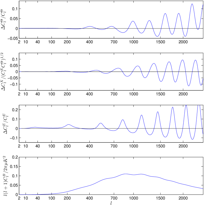
Figure 4: Difference between the lensed and unlensed temperature, cross-correlation and $E$-polarization power spectra (top three plots), and the lensed $B$ power spectrum (bottom) for a fiducial concordance model. The unlensed model has no tensor component (so no $B$-mode power), and the lensed $B$ power spectrum shown is not highly accurate due to the neglect of non-linear evolution in the lensing potential. The magnitude of the lensing effect depends on the fluctuation amplitude in the model; here the model has curvature perturbation power $A_{s}=2.5\times 10^{-9}$ on $0.05\,\text{Mpc}^{-1}$ scales and spectral index $n_{s}=0.99$.

The correlation function method is inherently very efficient, only requiring the evaluation of one dimensional sums and integrals. For an accurate calculation of $\tilde{C}_{l}^{B}$ it is essential to compute the full range of the correlation function because it is sensitive to large and small scales. However, when $\tilde{C}_{l}^{B}$ is not needed the lensing is only a small-scale effect and we only need to integrate some of the angular range to compute $\tilde{\xi}(\beta)-\xi(\beta)$ (and hence the lensing contribution $\tilde{C}_{l}-C_{l}$). We find that using $\beta_{\text{max}}=\pi/16$ is sufficient for $0.1\%$ accuracy to $l=2000$, providing a significant factor of 16 gain in speed. Truncating the correlation function does induce ringing on very small scales, so if accuracy is needed on much smaller scales the angular range can be increased. For all but very small scales, and the $\tilde{C}_{l}^{B}$ spectrum, we can accurately evaluate the sums over $l$ to compute the lensed correlation functions by sampling only every 10th $l$, yielding an additional significant time saving.

Our code is publicly available as part of camb, with execution time being dominated by that required to compute the transfer functions for the CMB and the lensing potential. Once these have been computed, the time required to compute the unlensed $C_{l}$ and then lens the result is about a hundred times less (if $\tilde{C}_{l}^{B}$ is not required accurately). This means that efficient methods for exploiting ‘fast’ and ‘slow’ parameters Lewis and Bridle (2002, ) during Markov Chain Monte Carlo parameter estimation can still be applied when lensing is accounted for via the lensed power spectrum.

Sample numerical results for the lensed CMB power spectra compared to the unlensed spectra are shown in Fig. 4.

IV Comparison of methods

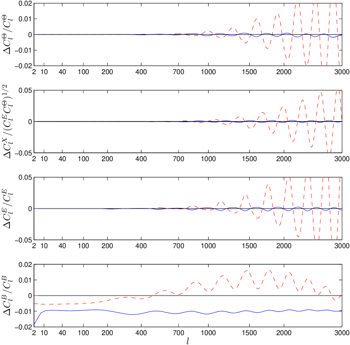
Figure 5: Comparison of our new result with the $O(C_{l}^{\psi})$ harmonic result of Ref. Hu (2000a) (dashed) and the flat-sky non-perturbative result of Ref. Seljak (1996), extended to second order in $C_{\text{gl},2}$ (solid). The magnitude of the difference depends on the exact model and we have neglected non-linear contributions to the lensing potential.

We are now in a position to compare our new, accurate full-sky result with previous work. In Fig. 5 we compare our result with the full-sky lowest-order perturbative harmonic result of Ref. Hu (2000a) [correct to $O(C_{l}^{\psi}{})$] for a typical concordance model. We also compare to the flat-sky result of Refs. Seljak (1996); Zaldarriaga and Seljak (1998a) which is non-perturbative in $\sigma^{2}$. [We extend their results to second order in $C_{\text{gl},2}$ using Eqs. (17) and (21)]. In all cases we use an accurate numerical calculation of $C_{l}^{\psi}$, rather than the Limber approximation, and ignore its non-linear contribution.

It is clear that the lowest-order perturbative harmonic method of Ref. Hu (2000a) is not sufficiently accurate for precision cosmology, with $\sim 1\%$ errors on the temperature and $\sim 5\%$ on the $E$-mode polarization by $l\sim 2000$. These errors are sufficient to bias parameters even with the planned Planck satellite observations. The perturbative harmonic result is equivalent to expanding the correlation function result self-consistently to first order in $C_{l}^{\psi}$. As discussed in Sec. III.2, this is inaccurate because $l^{2}\sigma^{2}$ in the isotropic terms is not very small for large $l$, so many terms need to be retained to get accurate results. It is possible to extend the harmonic result to higher order Cooray (2004), however the multi-dimensional integrals required scale exponentially badly with increasing order. Even a self-consistent expansion to second order in $C_{l}^{\psi}$ is not good enough at $l>2000$, so at least third order would be required. Furthermore we see that for $\tilde{C}_{l}^{B}$ the method is also somewhat inaccurate on large scales: because the $B$-mode signal comes from a wide range of $l$, and the $E$-mode power peaks on small scales, the non-perturbative effects can be significant on all scales. In fact, the large-scale lensed $E$-mode power also receives most of its contribution from small-scale modes since the unlensed polarization power spectrum rises steeply with $l$ on large scales. However, lensing is still only a small fractional effect for $E$-polarization on large scales and so the perturbative expansion is relatively more accurate for $E$ than $B$.

The correlation function methods can easily handle the isotropic term non-perturbatively. The accurate flat-sky result is much more accurate than the lowest-order harmonic full-sky result, with only $\sim 0.3\%$ curvature corrections to the temperature. The polarization errors are rather larger, with percent-level difference on $\tilde{C}_{l}^{B}$. Although this is smaller than the effect of non-linearities in the lensing potential (see Section V), the latter can be accurately accounted for with better modelling (e.g. Ref. Smith et al. (2003)) or simulations. While the accurate flat-sky result is probably sufficient to Planck sensitivities, curvature effects must be taken account for truly accurate results approaching the cosmic-variance limit. Although the curvature is negligible on the scale of the deflection angles, it is not negligible on the scale of the lensing potential coherence length. Computing our full-sky accurate result is not much harder or slower than computing the flat result, so we recommend our new calculation for future work.

Note that the absolute precision of the lensed results is limited by the accuracy of the computed lensing potential and the unlensed CMB power spectra. In particular, uncertainties in the ionization history may generate errors significantly above cosmic variance on the unlensed $C_{l}$. We use the recfast code of Ref. Seager et al. (2000) that may well be inaccurate at above the percent level Leung et al. (2004); Dubrovich and Grachev (2005). However if the ionization history can be computed reliably to high accuracy our new lensing method can then be used to compute the lensed power spectra accurately.

V Non-linear evolution

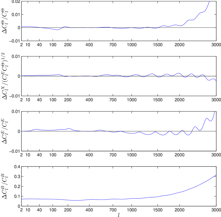
Figure 6: The fractional change in the lensed $C_{l}$ due to non-linear corrections using halofit Smith et al. (2003) for the same model as Fig. 4. The lensed $C_{l}$ are computed using our new accurate method.

The most important assumption we have made so far is that the lensing potential is linear and Gaussian. On small scales this will not be quite correct. Although our method does not allow us to account for the non-Gaussianity, we can take into account the effect of non-linear evolution on the power spectrum of the lensing potential [and hence $\sigma^{2}(\beta)$ and $C_{\text{gl},2}(\beta)$ Seljak (1996)]. On scales where the non-Gaussianity of the deflection field is small this should be a good approximation, assuming we have an accurate way to compute the non-linear power spectrum of the density field.

We use the halofit code of Ref. Smith et al. (2003) to compute an approximate non-linear, equal-time power spectrum given an accurate numerical linear power spectrum at a given redshift. halofit is expected to be accurate at the few percent level for standard $\Lambda$CDM models with power law primordial power spectra (but cannot be relied on for other models, for example with an evolving dark energy component). We simply scale the potential transfer functions $T_{\Psi}(k,\eta)$ of Eq. (5) so that the power spectrum of the potential $\Psi$ has the correct non-linear form at that redshift:

$$T_{\Psi}(k,\eta)\rightarrow T_{\Psi}(k,\eta)\sqrt{\frac{\mathcal{P}^{\text{non-linear}}_{\Psi}(k,\eta)}{\mathcal{P}_{\Psi}(k,\eta)}}.$$ (67)

Since non-linear effects on $C_{l}^{\psi}$ are only important where the Limber approximation holds, Eq. (67) should be very accurate.

The effect of the non-linear evolution on the power spectrum of the lensing potential is shown in Fig. 1. Although there is very little effect on scales where the power peaks ($l\sim 60$), non-linear evolution significantly increases the power on small scales. The corresponding changes to the lensed CMB power spectra are shown in Fig. 6. The temperature power spectrum $\tilde{C}_{l}^{\Theta}$ is changed by $\lesssim 0.2\%$ for $l\sim 2000$, but there are percent level changes on smaller scales. Thus inclusion of the non-linear evolution will be important to obtain results accurate at cosmic-variance levels, but is not likely to be important at $l<2000$ for the near future. The effect on the $B$-mode power spectrum is more dramatic, giving a $>6\%$ increase in power on all scales. On scales beyond the peak in the $B$-mode power ($l\gtrsim 1000$) the extra non-linear power becomes more important, producing an order unity change in the $B$-mode spectrum on small scales. On these scales the assumption of Gaussianity is probably not very good, and the accuracy will also be limited by the precision of the non-linear power spectrum. For more accurate results, more general models, and on very small scales where the non-Gaussianity of the lensing potential becomes important, numerical simulations may be required (e.g. see Refs. White and Vale (2004); White and Hu (2000)).

There are, of course, other non-linear effects on the CMB with the same frequency spectrum as the primordial (and lensed) temperature anisotropies and polarization. The kinematic Sunyaev-Zel’dovich (SZ) effect is the main such effect for the temperature anisotropies, and current uncertainties in the reionization history and morphology make the spectrum $C_{l}^{\Theta}$ uncertain at the few percent level at $l=2000$ Zahn et al. (2005). This is a little larger than the error in the first-order harmonic lensing result, but this doesn’t mean that one should be content with the error in the latter. Precision cosmology from the damping tail will require accurate modelling of both lensing and the kinematic SZ effect. Errors at the percent level in the lensing power on these scales would seriously limit our ability to constrain reionization scenarios with future arcminute-resolution observations. For the polarization spectra, the kinematic SZ effect is much less significant Hu (2000b).

VI Conclusions

We have presented a new, fast and accurate method for computing the lensed CMB power spectra using spherical correlation functions. Previous perturbative methods were found to be insufficiently inaccurate for precision cosmology, and non-perturbative results in the flat-sky approximation are in error at above the cosmic-variance level. The method developed here should enable accurate calculation of the lensing effect to within cosmic-variance limits to $l\lesssim 2500$ under the assumptions of the Born approximation and Gaussianity of the primordial fields. Non-linear corrections to the lensing potential have only a small effect on the lensed temperature power spectrum, but are important on all scales for an accurate calculation of the lensed $B$-mode power spectrum.

VII Acknowledgments

We thank Gayoung Chon for her work towards implementing the full-sky lowest-order lensing result of Ref. Hu (2000a) in camb, and AL thanks Matias Zaldarriaga, Mike Nolta, Oliver Zahn, Patricia Castro, Pat McDonald and Ben Wandelt for discussion and communication. AC acknowledges a Royal Society University Research Fellowship.

Appendix A Rotating spin-weight harmonics

Consider evaluating ${}_{s}Y_{lm}$ at $\hat{D}\hat{\mathbf{n}}$, where $\hat{D}$ is the rotation operator corresponding to Euler angles $\alpha$, $\beta$ and $\gamma$. This is the same as rigidly rotating the function ${}_{s}Y_{lm}$ (as a scalar) by $\hat{D}^{-1}$ and evaluating at $\hat{\mathbf{n}}$. For spin-0 harmonics we know that

$$Y_{lm}(\hat{D}\hat{\mathbf{n}})=D^{l}_{m^{\prime}m}(-\gamma,-\beta,-\alpha)Y_{lm^{\prime}}(\hat{\mathbf{n}}).$$ (68)

For spin-$s$ harmonics, we note that

$${}_{s}Y_{lm}(\hat{\mathbf{n}})=(-1)^{m}\sqrt{\frac{2l+1}{4\pi}}D^{l}_{-ms}(\phi,\theta,0),$$ (69)

where $(\theta,\phi)$ refer to $\hat{\mathbf{n}}$, so that

$$D^{l}_{m^{\prime}m}(-\gamma,-\beta,-\alpha){}_{s}Y_{lm^{\prime}}(\hat{\mathbf{n}}) = (-1)^{m^{\prime}}\sqrt{\frac{2l+1}{4\pi}}D^{l}_{m^{\prime}m}(-\gamma,-\beta,-\alpha)D^{l}_{-m^{\prime}s}(\phi,\theta,0)$$ (70)

$$= (-1)^{m}\sqrt{\frac{2l+1}{4\pi}}D^{l}_{-mm^{\prime}}(\alpha,\beta,\gamma)D^{l}_{m^{\prime}s}(\phi,\theta,0)$$

$$= (-1)^{m}\sqrt{\frac{2l+1}{4\pi}}D^{l}_{-ms}(\phi^{\prime},\theta^{\prime},\kappa)$$

$$= {}_{s}Y_{lm}(\hat{D}\hat{\mathbf{n}})e^{-is\kappa}.$$

Here, we have used $\hat{D}(\alpha,\beta,\gamma)\hat{D}(\phi,\theta,0)=\hat{D}(\phi^{\prime},\theta^{\prime},\kappa)$, so that $(\theta^{\prime},\phi^{\prime})$ refer to the image of $\hat{\mathbf{n}}$ under $\hat{D}(\alpha,\beta,\gamma)$, and $\kappa$ is the additional rotation required about $\hat{D}\hat{\mathbf{n}}$ to map the polar basis vectors there onto the image of the polar basis at $\hat{\mathbf{n}}$ under $\hat{D}(\alpha,\beta,\gamma)$. Denoting the polar basis (unit) vectors at $\hat{\mathbf{n}}$ by $\mathbf{e}_{\theta}$ and $\mathbf{e}_{\phi}$, and at $\hat{\mathbf{n}}^{\prime}$ by $\mathbf{e}_{\theta}^{\prime}$ and $\mathbf{e}_{\phi}^{\prime}$, we have

$$\mathbf{e}_{\theta}^{\prime}\pm i\mathbf{e}_{\phi}^{\prime}=e^{\pm i\kappa}\hat{D}(\mathbf{e}_{\theta}\pm i\mathbf{e}_{\phi}).$$ (71)

This ensures that the $2l+1$ rank-$s$ tensor fields ${}_{\pm}\mathbf{Y}_{lm}(\hat{\mathbf{n}})\equiv{}_{\pm s}Y_{lm}(\hat{\mathbf{n}})(\mathbf{e}_{\theta}\mp i\mathbf{e}_{\phi})\otimes\cdots\otimes(\mathbf{e}_{\theta}\mp i\mathbf{e}_{\phi})$ transform irreducibly under rotations as $\hat{D}{}_{\pm}\mathbf{Y}_{lm}=\sum_{m^{\prime}}D^{l}_{m^{\prime}m}{}_{\pm}\mathbf{Y}_{lm^{\prime}}$.

Appendix B Evaluation of $X_{imn}$

The integrals

$$X_{imn}\equiv\int_{0}^{\infty}\frac{2\alpha}{\sigma^{2}}\left(\frac{\alpha}{\sigma^{2}}\right)^{i}e^{-\alpha^{2}/\sigma^{2}}d^{l}_{mn}(\alpha)\,{\text{d}}\alpha$$ (72)

that are required for the non-perturbative calculation of the lensed power spectra on the spherical sky can easily be evaluated as series in $\sigma^{2}$. From the definition of the rotation matrices, we have

$$d^{l}_{mn}(\alpha)=\langle lm|e^{-i\alpha\hat{L}_{y}}|ln\rangle,$$ (73)

where we adopt the Condon–Shortley phase for the eigenstates $|lm\rangle$ of the $\hat{L}_{z}$ and $\hat{L}^{2}$ angular momentum operators, and we have set $\hbar=1$. Expanding the exponential as a series in $\alpha$, we have

$$X_{imn}=\sum_{j=0}^{\infty}\frac{1}{j!}\sigma^{j-i}\Gamma(j+1+i/2)\langle lm|(-i\hat{L}_{y})^{j}|ln\rangle.$$ (74)

The action of the $\hat{L}_{y}$ operator on the eigenstates of $\hat{L}_{z}$ is given by the familiar result

$$-i\hat{L}_{y}|lm\rangle={\textstyle{\frac{1}{2}}}\sqrt{l(l+1)-m(m-1)}|l\,m-1\rangle-{\textstyle{\frac{1}{2}}}\sqrt{l(l+1)-m(m+1)}|l\,m+1\rangle,$$ (75)

and this can be used recursively to evaluate the matrix element in Eq. (74).

For $l\gg 1/\sigma$ the series in Eq. (74) is slow to converge and a non-perturbative treatment of the $X_{imn}$ is required. Using the asymptotic result

$$d^{l}_{mn}(\alpha)\sim(-1)^{n-m}J_{m-n}[(l+1/2)\alpha],$$ (76)

valid for $l\rightarrow\infty$ with $l\alpha\gg 1$ but $\alpha\ll 1$, and, noting that we only require the case $i=m-n$, we can use Eq. (6.6314) from Ref. Gradshteyn and Ryzhik (2000) to show that

$$X_{imn}\sim\left(-\frac{(l+1/2)}{2}\right)^{i}e^{-(l+1/2)^{2}\sigma^{2}/4}\quad\mbox{for $i=m-n$}.$$ (77)

In practice, we obtain an excellent approximation to $X_{imn}$, valid for all $l$, by adjusting the $l$-independent term in the exponent of the asymptotic result, and the prefactor, so that its series expansion agrees with a direct evaluation of Eq. (74) to $O(\sigma^{2})$.

Appendix C Full second order result

The full result for the lensed correlation functions accurate to second order in $C_{\text{gl}}$ and $C_{\text{gl},2}$ is

$$\tilde{\xi} \approx\sum_{l}\frac{2l+1}{4\pi}C^{\Theta}_{l}\biggl{\{}\left(X_{000}^{2}+2C_{\text{gl}}X_{000}X_{000}^{\prime}+C_{\text{gl}}^{2}(X_{000}^{\prime\prime}X_{000}+2X_{000}^{\prime\,2})+C_{\text{gl},2}^{2}X_{000}^{\prime\,2}\right)d_{00}^{l}$$

$$\hskip 85.35826pt+\frac{8}{l(l+1)}X_{000}^{\prime}\left(X_{000}^{\prime}+2C_{\text{gl}}X_{000}^{\prime\prime}\right)\left(C_{\text{gl},2}d_{1-1}^{l}+C_{\text{gl}}d_{11}^{l}\right)+C_{\text{gl},2}^{2}X_{220}^{2}d_{2-2}^{l}$$

$$\hskip 85.35826pt+C_{\text{gl}}^{2}X_{220}^{2}d_{22}^{l}-4C_{\text{gl}}C_{\text{gl},2}X_{000}^{\prime}X_{220}d_{20}^{l}\biggr{\}}$$ (78)

$$\tilde{\xi}_{+} \approx\sum_{l}\frac{2l+1}{4\pi}(C^{E}_{l}+C^{B}_{l})\biggl{\{}\left(X_{022}^{2}+2C_{\text{gl}}X_{022}X_{022}^{\prime}+C_{\text{gl}}^{2}(X_{022}^{\prime\prime}X_{022}+2X_{022}^{\prime\,2})+C_{\text{gl},2}^{2}X_{022}^{\prime\,2}\right)d_{22}^{l}$$

$$\hskip 142.26378pt+C_{\text{gl}}X_{132}(X_{132}+2C_{\text{gl}}X_{132}^{\prime})d_{33}^{l}+C_{\text{gl}}X_{121}(X_{121}+2C_{\text{gl}}X_{121}^{\prime})d_{11}^{l}$$

$$\hskip 142.26378pt+2C_{\text{gl},2}\left[X_{121}X_{132}+C_{\text{gl}}(X_{121}X_{132}^{\prime}+X_{132}X_{121}^{\prime})\right]d_{31}^{l}+\frac{1}{2}C_{\text{gl}}^{2}X_{220}^{2}d_{00}^{l}$$

$$\hskip 142.26378pt+C_{\text{gl},2}^{2}X_{220}X_{242}d_{40}^{l}-2C_{\text{gl}}C_{\text{gl},2}(X_{220}X_{022}^{\prime}d_{20}^{l}+X_{242}X_{022}^{\prime}d_{42}^{l})+\frac{1}{2}C_{\text{gl}}^{2}X_{242}^{2}d_{44}^{l}\biggr{\}}$$ (79)

$$\tilde{\xi}_{-} \approx\sum_{l}\frac{2l+1}{4\pi}(C^{E}_{l}-C^{B}_{l})\biggl{\{}\left(X_{022}^{2}+2C_{\text{gl}}X_{022}X_{022}^{\prime}+C_{\text{gl}}^{2}(X_{022}^{\prime\prime}X_{022}+2{X_{022}^{\prime}}^{2})+C_{\text{gl},2}^{2}{X_{022}^{\prime}}^{2}\right)d_{2-2}^{l}$$

$$\hskip 142.26378pt+C_{\text{gl},2}X_{132}(X_{132}+2C_{\text{gl}}X_{132}^{\prime})d_{3-3}^{l}+C_{\text{gl},2}X_{121}(X_{121}+2C_{\text{gl}}X_{121}^{\prime})d_{1-1}^{l}$$

$$\hskip 142.26378pt+2C_{\text{gl}}\left(X_{121}X_{132}+C_{\text{gl}}[X_{121}X_{132}^{\prime}+X_{132}X_{121}^{\prime}]\right)d_{3-1}^{l}+\frac{1}{2}C_{\text{gl},2}^{2}X_{220}^{2}d_{00}^{l}$$

$$\hskip 142.26378pt+C_{\text{gl}}^{2}X_{220}X_{242}d_{40}^{l}-2C_{\text{gl}}C_{\text{gl},2}(X_{220}X_{022}^{\prime}d_{20}^{l}+X_{242}X_{022}^{\prime}d_{4-2}^{l})+\frac{1}{2}C_{\text{gl},2}^{2}X_{242}^{2}d_{4-4}^{l}\biggr{\}}$$ (80)

$$\tilde{\xi}_{X} \approx\sum_{l}\frac{2l+1}{4\pi}C^{X}_{l}\biggl{\{}\biggl{[}X_{022}X_{000}+C_{\text{gl}}(X_{022}X_{000}^{\prime}+X_{000}X_{022}^{\prime})+C_{\text{gl},2}^{2}(X_{000}^{\prime}X_{022}^{\prime}+\frac{1}{2}X_{220}^{2})$$

$$\hskip 170.71652pt+\frac{1}{2}C_{\text{gl}}^{2}(X_{220}^{2}+X_{000}X_{022}^{\prime\prime}+X_{022}X_{000}^{\prime\prime}+4X_{022}^{\prime}X_{000}^{\prime})\biggr{]}d_{20}^{l}$$

$$\hskip 85.35826pt+\frac{2}{\sqrt{l(l+1)}}\left[C_{\text{gl}}(X_{121}X_{000}^{\prime\prime}+X_{121}^{\prime}X_{000}^{\prime})+X_{121}X_{000}^{\prime}\right]\left(C_{\text{gl}}d_{1-1}^{l}+C_{\text{gl},2}d_{11}^{l}\right)$$

$$\hskip 85.35826pt+\frac{2}{\sqrt{l(l+1)}}\left[C_{\text{gl}}(X_{132}X_{000}^{\prime\prime}+X_{132}^{\prime}X_{000}^{\prime})+X_{132}X_{000}^{\prime}\right]\left(C_{\text{gl},2}d_{3-1}^{l}+C_{\text{gl}}d_{31}^{l}\right)$$

$$\hskip 85.35826pt-C_{\text{gl}}C_{\text{gl},2}(X_{000}^{\prime}X_{220}d_{00}^{l}+X_{000}^{\prime}X_{242}d_{40}^{l})+\frac{1}{2}X_{242}X_{220}(C_{\text{gl},2}^{2}d_{4-2}^{l}+C_{\text{gl}}^{2}d_{42}^{l})\biggl{\}}.$$ (81)

As discussed in the main text, the $C_{\text{gl}}$ terms may be neglected at the $O(10^{-4})$ level for realistic lensing deflection amplitudes.

References

- Seljak (1996) U. Seljak, Astrophys. J. 463, 1 (1996), eprint astro-ph/9505109.
- Zaldarriaga and Seljak (1998a) M. Zaldarriaga and U. Seljak, Phys. Rev. D58, 023003 (1998a), eprint astro-ph/9803150.
- Hu (2000a) W. Hu, Phys. Rev. D62, 043007 (2000a), eprint astro-ph/0001303.
- Seljak and Zaldarriaga (1999) U. Seljak and M. Zaldarriaga, Phys. Rev. Lett. 82, 2636 (1999), eprint astro-ph/9810092.
- Guzik et al. (2000) J. Guzik, U. Seljak, and M. Zaldarriaga, Phys. Rev. D62, 043517 (2000), eprint astro-ph/9912505.
- Hu (2001) W. Hu, Astrophys. J. 557, L79 (2001), eprint astro-ph/0105424.
- Hu and Okamoto (2002) W. Hu and T. Okamoto, Astrophys. J. 574, 566 (2002), eprint astro-ph/0111606.
- Hirata and Seljak (2003) C. M. Hirata and U. Seljak, Phys. Rev. D68, 083002 (2003), eprint astro-ph/0306354.
- Smith et al. (2004) K. M. Smith, W. Hu, and M. Kaplinghat, Phys. Rev. D70, 043002 (2004), eprint astro-ph/0402442.
- Lewis (2005) A. Lewis (2005), eprint astro-ph/0502469.
- Seljak and Zaldarriaga (2000) U. Seljak and M. Zaldarriaga, Astrophys. J. 538, 57 (2000), eprint astro-ph/9907254.
- Challinor and Chon (2002) A. Challinor and G. Chon, Phys. Rev. D66, 127301 (2002), eprint astro-ph/0301064.
- Lewis et al. (2000) A. Lewis, A. Challinor, and A. Lasenby, Astrophys. J. 538, 473 (2000), eprint astro-ph/9911177.
- Zaldarriaga and Seljak (1998b) M. Zaldarriaga and U. Seljak, Phys. Rev. D58, 023003 (1998b), eprint astro-ph/9803150.
- Zaldarriaga and Seljak (1997) M. Zaldarriaga and U. Seljak, Phys. Rev. D55, 1830 (1997), eprint astro-ph/9609170.
- Lewis et al. (2002) A. Lewis, A. Challinor, and N. Turok, Phys. Rev. D65, 023505 (2002), eprint astro-ph/0106536.
- Chon et al. (2004) G. Chon, A. Challinor, S. Prunet, E. Hivon, and I. Szapudi, Mon. Not. Roy. Astron. Soc. 350, 914 (2004), eprint astro-ph/0303414.
- Lewis and Bridle (2002) A. Lewis and S. Bridle, Phys. Rev. D66, 103511 (2002), eprint astro-ph/0205436.
- (19) A. Lewis and S. Bridle, http://cosmologist.info/notes/cosmomc.ps.gz.
- Cooray (2004) A. R. Cooray, New Astron. 9, 173 (2004), eprint astro-ph/0309301.
- Smith et al. (2003) R. E. Smith et al. (The Virgo Consortium), Mon. Not. Roy. Astron. Soc. 341, 1311 (2003), eprint astro-ph/0207664.
- Seager et al. (2000) S. Seager, D. D. Sasselov, and D. Scott, Astrophys. J. Suppl. 128, 407 (2000), eprint astro-ph/9912182.
- Dubrovich and Grachev (2005) V. K. Dubrovich and S. I. Grachev (2005), eprint astro-ph/0501672.
- Leung et al. (2004) P. K. Leung, C.-W. Chan, and M.-C. Chu, Mon. Not. Roy. Astron. Soc. 349, 632 (2004), eprint astro-ph/0309374.
- White and Vale (2004) M. J. White and C. Vale, Astropart. Phys. 22, 19 (2004), eprint astro-ph/0312133.
- White and Hu (2000) M. J. White and W. Hu, Astrophys. J. 537, 1 (2000), eprint astro-ph/9909165.
- Zahn et al. (2005) O. Zahn, M. Zaldarriaga, L. Hernquist, and M. McQuinn (2005), eprint astro-ph/0503166.
- Hu (2000b) W. Hu, Astrophys. J. 529, 12 (2000b), eprint astro-ph/9907103.
- Gradshteyn and Ryzhik (2000) I. S. Gradshteyn and I. M. Ryzhik, Table of Integrals, Series and Products, 6th edn. (Academic Press, San Diego, 2000).