GEMS: The Size Evolution of Disk Galaxies

Abstract

We combine HST imaging from the GEMS survey with photometric redshifts from COMBO-17 to explore the evolution of disk-dominated galaxies since $z\lesssim 1.1$. The sample is comprised of all GEMS galaxies with Sérsic indices $n<2.5$, derived from fits to the galaxy images. We account fully for selection effects through careful analysis of image simulations; we are limited by the depth of the redshift and HST data to the study of galaxies with $M_{V}\lesssim-20$, or equivalently $\log\left(\mathcal{M}/\mathcal{M}_{\odot}\right)\gtrsim 10$. We find strong evolution in the magnitude–size scaling relation for galaxies with $M_{V}\lesssim-20$, corresponding to a brightening of $\sim$1 mag arcsec^-2 in rest-frame $V$-band by $z\sim 1$. Yet, disks at a given absolute magnitude are bluer and have lower stellar mass-to-light ratios at $z\sim 1$ than at the present day. As a result, our findings indicate weak or no evolution in the relation between stellar mass and effective disk size for galaxies with $\log\left(\mathcal{M}/\mathcal{M}_{\odot}\right)\gtrsim 10$ over the same time interval. This is strongly inconsistent with the most naive theoretical expectation, in which disk size scales in proportion to the halo virial radius, which would predict that disks are a factor of two denser at fixed mass at $z\sim 1$. The lack of evolution in the stellar mass–size relation is consistent with an “inside-out” growth of galaxy disks on average (galaxies increasing in size as they grow more massive), although we cannot rule out more complex evolutionary scenarios.

1. Introduction

The last eight billion years have witnessed strong evolution of the disk galaxy population. Both ‘archaeological’ studies of local disk-dominated galaxies and ‘look-back’ studies of the evolution of disk galaxies suggest a steady build-up in their stellar masses since $z\sim 1$ (Rocha-Pinto et al., 2000; Flores et al., 1999; Bell et al., 2005; Hammer et al., 2005). Insights into how this growth occurs are accessible through the study of disk galaxy scaling relations, such as the luminosity–rotation velocity (Tully-Fisher) relation or the luminosity–size relation (e.g. Vogt et al., 1996; Lilly et al., 1998; Simard et al., 1999; Böhm et al., 2004). Yet, owing to sample size limitations, selection effects, and differences in analysis techniques, these studies have come to widely divergent conclusions. In this paper, we explore the evolution of the luminosity–size and stellar mass–size relations over the last 8 Gyr (since $z\sim 1$) using a sample of almost 5700 disk-dominated galaxies from the HST GEMS survey (Galaxy Evolution from Morphology and SEDs Rix et al., 2004).

In the Cold Dark Matter (CDM) picture of structure formation, collapsing dark matter perturbations acquire angular momentum through tidal torques and mergers (Peebles, 1969; Maller et al., 2002; Vitvitska et al., 2002). Some fraction of this angular momentum is conserved, leading to the formation of cold, rotationally-supported disks. The typical magnitude of the specific angular momentum predicted in this framework leads to the formation of present day disks with approximately the correct distribution of radial sizes, if the specific angular momentum of the gas is similar to that of the dark matter and is mostly conserved during the formation process (Fall & Efstathiou, 1980).

A difficulty is that this idealized picture does not correspond to the outcome when the process of galaxy formation is simulated in detail within the cosmological context of CDM. In hydrodynamical simulations, the gas tends to lose a large fraction of its initial angular momentum, resulting in disks that are too small compared to observed nearby galaxies (Navarro & White, 1994; Sommer-Larsen et al., 1999; Navarro & Steinmetz, 2000; D’Onghia & Burkert, 2004). Furthermore, very few ‘late-type’ disks are formed in such simulations: galaxies tend to suffer mergers that thicken and destroy their disks (Steinmetz & Navarro, 2002). It is not yet established whether this problem represents a fundamental difficulty with the ‘standard’ CDM paradigm (i.e., a result of excess small scale power), a reflection of our incomplete ability to understand and simulate the complexities of star formation and supernova feedback, or inadequacies in numerical resolution.

Many proposed solutions to this problem involve delaying gas collapse and disk formation to later times, either by adopting an alternate power spectrum with reduced small scale power (such as Warm Dark Matter), in which structure formation occurs later (e.g. Sommer-Larsen & Dolgov, 2001), or by invoking some form of feedback that prevents the gas from cooling until relatively late times $z\sim 1$ (Weil et al., 1998; Thacker & Couchman, 2001). While these solutions would be consistent with an important build-up in the disk galaxy population at late times, the late formation times implied by these models may be in conflict with the old ages of disk stars in the Milky Way and M31 (Rocha-Pinto et al., 2000; Ferguson & Johnson, 2001). Additional constraints can be gleaned from so-called ‘backwards evolution’ models, in which the ages and metallicities of the stars in present-day disk galaxies are used to constrain the formation history of different components within our and other galaxies (Chiappini et al., 1997; Boissier & Prantzos, 1999). Direct measurements of the mass–size scaling relations and radial size distributions of disk galaxies at earlier epochs will provide an important counterpoint to these arguments by providing direct constraints on the angular momentum content of stars at these earlier times.

A number of previous studies have used the Hubble Space Telescope (HST) to quantify the evolution of disk galaxies by measuring their absolute sizes and magnitudes as a function of redshift. Magnitude and size are strongly correlated; a line of constant surface brightness falls almost parallel to the distribution of observed galaxies, making the evolution of galaxy surface brightness a natural choice for parameterizing the evolution of galaxy sizes. However, the results of studies measuring average rest-frame surface brightnesses as a function of redshift have proven controversial, ranging from detecting no evolution to rather strong evolution in the range of 1-2 mag arcsec^-2 brightening by redshift $z\sim 1$. For example, Lilly et al. (1998) found an average increase of the surface brightness of $\sim 1$ mag by redshift $z\sim 1$. This result is supported by observations of galaxies at high redshifts ($z\sim 2-3$), detected in very deep ground-based near-infrared images (Labbé et al., 2003). Trujillo et al. (2004) estimate that the average rest-frame surface brightness of these objects is more than 2-3 mag arcsec^-2 brighter than in the local universe.

Simard et al. (1999) pointed out that selection effects play a crucial role in such analyses. After accounting for the different sources of incompleteness, Simard et al. (1999) and Ravindranath et al. (2004) argue that the luminosity–size relation of disk galaxies evolves by less than 0.4 mag arcsec^-2 over the interval $0.25<z<1.25$. Yet, in order to reproduce the observations, both groups found it necessary to introduce a new population of high surface brightness galaxies in the highest redshift bin ($z\sim 1$). A different interpretation was suggested by Trujillo & Aguerri (2004), who find strong evolution of the average rest-frame $V$-band surface brightness of $\sim 0.8$ mag arcsec^-2 at a redshift $z\sim 0.7$, also including a full treatment of completeness.

In this work, we present the results from a new sample of disk-dominated galaxies from the GEMS survey. Each of our galaxies has a spectrophotometrically-measured redshift, a spectral energy distribution (Wolf et al., 2004, SED), and a stellar mass estimate (Borch, 2004) from COMBO-17 . We combine these SED constraints with light-profile shapes and sizes determined from deep high-resolution HST Advanced Camera for Surveys (ACS) images. We reassess the evolution of the magnitude–size and stellar mass–size relation as a function of redshift over the range $0.1\lesssim z\lesssim 1.1$, taking particular care to model the impact of the selection function. We suggest a resolution to the conflicting previous results by presenting a coherent picture of strong surface brightness evolution with redshift without the need for a new population of high surface brightness galaxies.

The layout of this paper is as follows. In $\S$ 2 we present the GEMS data set and describe the sample selection, the galaxy fitting techniques and the corrections we applied to the data. We explain in some more detail our modeling of the sample completeness in $\S$ 3. In $\S$ 4, we explore the evolution of the magnitude–size and stellar mass–size relations for disk-dominated galaxies. We show that there is a trend of increasing average surface brightness with redshift and that there is little evolution of the surface mass density. In $\S$ 5 we discuss our results in comparison with previous studies in the literature, and compare them with theoretical expectations. We summarize our results in $\S$ 6. Throughout this paper we use the concordance cosmology with $H_{0}=70$ km s^-1 Mpc^-1, $\Omega_{M}=0.3$ and $\Omega_{\Lambda}=0.7$ (Spergel et al., 2003). Unless indicated otherwise we use Vega-normalized magnitudes.

2. Sample Definition

2.1. Imaging Data

GEMS, Galaxy Evolution from Morphologies and SEDs (Rix et al., 2004), has imaged an area of $\sim 800$ arcmin² centred on the Chandra Deep Field South (CDFS), using the ACS on-board HST. Of these 78 ACS tiles the central 15 were incorporated from the GOODS project (Giavalisco et al., 2004). With integration times of $\sim 35$ min in each of two filters (F606W and F850LP) the point source detection limits reached $m_{\textrm{\tiny{AB}}}\left(\textrm{F606W}\right)=28.3$ ($5\sigma$) and $m_{\textrm{\tiny{AB}}}\left(\textrm{F850LP}\right)=27.1$ ($5\sigma$), respectively. Details about the image mosaic and data reduction will be explained in a subsequent paper (Caldwell et al. 2005, in prep.).

2.2. COMBO-17 Data

The HST imaging data is complemented by low resolution spectrophotometric data from COMBO-17 (Wolf et al., 2004). COMBO-17 has provided precise redshift estimates ($\sigma_{z}/(1+z)\sim 0.02$) for approximately 9000 galaxies down to $m_{R}<24$. Rest-frame absolute magnitudes and colors, accurate to $\sim$0.1 mag, are also available for these galaxies. Furthermore, using a simple parameterized star formation history and the photometry in the 17 COMBO-17 bands, Borch (2004) computed stellar mass estimates for each galaxy in our sample, assuming a Kroupa et al. (1993) stellar initial mass function (IMF). These mass estimates are consistent with those derived using a one-color-based transformation from light to mass as described in Bell & de Jong (2001) and Bell et al. (2003). While such estimates suffer from uncertainties in the IMF, ages, dust, and metallicity, it is encouraging to note that several studies (Bell et al., 2003; Drory et al., 2004) find good agreement between masses based on broad-band colors and those from spectroscopic (e.g. Kauffmann et al., 2003a, b) and dynamical (Drory et al., 2004) techniques.

2.3. Source Detection

For source detection we use the SExtractor software (Bertin & Arnouts, 1996) on the F850LP image. In contrast to the standard single-pass approach, we apply a two-step process, running SExtractor twice on each image to find an acceptable compromise between deblending and detection threshold (see Rix et al., 2004). Combining the source lists from each tile, taking care to remove duplicate objects that were detected in two neighbouring tiles, we end up with over 40,000 galaxies.

2.4. Galaxy Fitting and Disk Selection

For the purpose of this paper we wish to isolate the subset of galaxies whose light is dominated by a disk component. We start by identifying all galaxies that can be reasonably well-fit by any single Sérsic profile (Sérsic, 1968) using the two-dimensional fitting code galfit (Peng et al., 2002). The Sérsic profile is a generalisation of a de Vaucouleurs profile with variable Sérsic index $n$:

$$\Sigma\left(R\right)=\Sigma_{e}\times\exp\left(-\kappa\left[\left(R/R_{e}\right)^{1/n}-1\right]\right),$$ (1)

where $R_{e}$ is the effective or half-light radius, $\Sigma_{e}$ is the effective surface density, $\Sigma\left(R\right)$ is the surface density as a function of radius and $\kappa=\kappa\left(n\right)$ is a normalization constant. An exponential profile has $n=1$ while a de Vaucouleurs profile has $n=4$. galfit convolves Sérsic profile galaxy models with the point spread function of the ACS (Jahnke et al., 2004, Jahnke et al., in preparation) and then determines the best fit by comparing the convolved models with the science data using a Levenberg-Marquardt algorithm to minimize the $\chi^{2}$ of the fit. The best-fit model is given by 7 parameter values and their associated uncertainties, including the half-light radius, the Sérsic index and the total magnitude. Initial galfit starting guesses for the model parameters were obtained from the SExtractor source catalogues. Typically, neighbouring galaxies were excluded from each model fit using a mask, but in the case of closely neighbouring galaxies with overlapping isophotes the galaxies were fitted simultaneously. The sky level for each galaxy was carefully measured using flux growth curves, masking out detected neighbouring sources. Lacking an estimate for the Sérsic index from SExtractor, we started all fits with $n=1.5$. In addition, all galaxies with $0.65<z<0.75$ were fitted with gim2d (Simard et al., 2002). Estimates for magnitudes, sizes and Sérsic indices from the two codes agree very well (see Bell et al. 2004; Häußler et al. 2005, in prep.). Morphological quantities quoted in the present paper were derived using galfit.

For this study, we estimate structural and morphological parameters from the $z$-band images (F850LP). In the optical (and the near-infrared), young stars make a progressively smaller contribution with increasing wavelength. Therefore, galaxy morphologies in F850LP are smoother than those in F606W, leading to a more robust detection and deblending of extended sources. The F850LP band corresponds to rest-frame $R$, $V$, and $B$-bands at $z\sim 0.4$, 0.7, and 1 respectively.

Selection of a galaxy sample for this kind of study is a multi-step process. First we merge the GEMS catalogue with the COMBO-17 redshift catalogue, then we select disk-dominated objects, and finally we remove sources with poor fits (see Fig. 1). We start by matching the GEMS sources to the COMBO-17 catalogue. To account for the relatively high source density in the GEMS images we pick the closest neighbour in the COMBO-17 catalogue within 0.5 arcsec as the corresponding match for a GEMS galaxy. Only at matching distances exceeding 1 arcsec does one start to include uncorrelated pairs. We are left with about 8000 matched sources in our sample.

We isolate disk-dominated galaxies for further study by cutting the sample based on the Sérsic profile fits. We adopt $n=2.5$ as the dividing line between disk- ($n<2.5$) and spheroid-dominated ($n>2.5$) galaxies. This cut discriminated between visually-classified early- and late-type galaxies from GEMS with $0.65<z<0.75$ with 80% reliability and less than 25% contamination (Bell et al., 2004). This cut is also consistent with the analysis conducted by the Sloan Digital Sky Survey (SDSS; see Shen et al., 2003). Furthermore, Ravindranath et al. (2004) have redshifted a sample of local galaxies to show that the Sérsic index is still a useful indicator at redshifts $z\sim 0.5-1$. Selecting galaxies with $n<2.5$ left us with $\sim 6200$ disk-dominated objects.

To ensure that the extracted galaxy profile parameters are reliable we remove objects from our source list that have relative formal errors in Sérsic index $n$ and effective radius $R_{e}$ of more than 25% ($\delta n/n>0.25$, $\delta R_{e}/R_{e}>0.25$). We also exclude objects that reach the boundary conditions for $n$ ($0.2<n<8$) or $R_{e}$ ($0.3<R_{e}$ [pixel] $<500$). Furthermore, we require that the galfit magnitudes coincide with the SExtractor magnitudes to within 0.6 mag ($|m_{\textrm{\tiny{GALFIT}}}-m_{\textrm{\tiny{SEx}}}+0.166|<0.6$). Finally, we remove compact sources with $\log R_{e}^{\textrm{\tiny{app}}}<\textrm{max}\left[8-0.4\times m_{z},0\right]$ (indicated by the solid line in the bottom left panel in Fig. 1). While slightly more galaxies with low surface brightness were removed by these additional cuts than high surface brightness galaxies, no pronounced bias was introduced. It is important to note that the simulated galaxy samples were also subjected to these same cuts for the construction of the completeness maps; thus, the completeness maps account fully for any biases introduced by these (necessary) extra sample cuts.

This sample selection should provide a fair representation of the disk-dominated galaxy population at all redshifts. The final catalogue contains 5664 disk galaxies with absolute rest-frame $B$- and $V$-band magnitudes, redshifts and stellar masses obtained from COMBO-17 and apparent half-light radii and Sérsic indices from galfit.

2.5. The Local Comparison Sample

In order to compare our measurements to a local reference point we have opted to use the NYU Value-Added Galaxy Catalog (VAGC; Blanton et al., 2004), which is based on the second data release (DR2) of the SDSS (Abazajian et al., 2004). It contains Sérsic fits for 28089 galaxies in the redshift range $0.0033<z<0.05$. For this paper, we use the VAGC elliptical aperture Sérsic fits for estimates of $r_{AB}$-band half-light radius, Sérsic index and -flux; coupled with extrapolated circular aperture $u_{AB},g_{AB},r_{AB},i_{AB},z_{AB}$ fluxes. The magnitudes were converted to absolute galactic foreground extinction-corrected magnitudes using the latest K-Correct routines, which were also used for the original data (Blanton et al., 2003). We apply the following correction to convert the SDSS elliptical half-light $r_{AB}$-band sizes to rest-frame $V$-band (see $\S$ 2.6): $R_{e}\left(V\right)=R_{e}\left(r\right)\times 1.011$. The redshift of the individual SDSS sources does not impact significantly on this correction factor. To obtain a rest-frame $B$-band size for the SDSS galaxies we use: $R_{e}\left(B\right)=R_{e}\left(V\right)\times 1.017$.

We have chosen the VAGC rather than the fits to the magnitude–size and stellar mass–size planes by Shen et al. (2003) for various reasons. Using the VAGC we have full control over all estimated parameters including the photometric system, k-corrections, etc. Specificially, the fits by Shen et al. (2003) where performed on circularized size estimates while we use elliptical Sérsic measurements. The half-light sizes and absolute magnitudes by Shen et al. (2003) were provided only in SDSS filters, necessitating the use of color transformations and of additional luminosity function convolutions in order to obtain mean values for the same selection and photometric system as the GEMS data. Furthermore, the VAGC allows us to repeat the same analysis procedure that was also used for the GEMS data. Finally, the VAGC incorporates the latest version of the SDSS pipeline, leading to more robust Sérsic indices, fainter apparent limiting magnitudes and fewer problems with deblending large sources. Since the VAGC and the data used by Shen et al. (2003) have $\sim 20,000$ sources in common we could verify that the measured parameters broadly agree with each other.

The VAGC does not contain stellar masses. Therefore, we have used the prescription given in Bell et al. (2003) to convert a $\left(g-r\right)_{AB}$ color into a SDSS $r_{AB}$-band stellar mass-to-light ratio:

$$\log\left(\mathcal{M}/L_{r}\right)=-0.306+1.097\times\left(g-r\right)_{AB}-0.15.$$ (2)

We have applied a correction of $-$0.15 to convert to a Kroupa IMF, in accord with our GEMS stellar masses. The stellar mass was then obtained from the following relation:

$$\log\left(\mathcal{M}\right)=\log\left(\mathcal{M}/L_{r}\right)-0.4\times\left(M_{r,S}-r_{\odot}\right),$$ (3)

with the absolute rest-frame Sérsic magnitude $M_{r,S}=r_{S}-5\log\left(D_{L}\right)-25$, the apparent rest-frame Sérsic magnitude $r_{S}$, the luminosity distance $D_{L}$ and the absolute magnitude of the sun $r_{\odot}=4.67$ in SDSS $r_{AB}$. Calculating a stellar mass in the same fashion for the lowest redshift GEMS galaxies and comparing this estimate with the SED-based masses (Borch, 2004) reveals no apparent systematic offsets.

2.6. Rest-Frame $V$-band Sizes

Galaxies are known to exhibit radial color gradients. As a result of this, galaxy sizes vary as a function of wavelength and the measured physical size evolution of the galaxy population could be skewed by the effects of band shifting with redshift. Therefore, we have not simply converted our apparent half-light sizes $R_{e}^{\textrm{\tiny{app}}}$ measured in the F850LP filter to a physical value, but instead have applied a color gradient correction to each individual galaxy according to its redshift to correct the size to the rest-frame $V$-band. For a sample of local galaxies, de Jong (1996) presents the relative disk scale lengths, which for a pure disk corresponds to $R_{e}=1.678\times R_{d}$, in the $B$-, $V$-, $R$-, $I$-, $H$- and $K$-bands. Figure 2 illustrates this ratio of the disk scale lengths in one band to the size measured in the $V$-band, as a function of the corresponding wavelength. A linear fit with the intercept fixed to 1 at the $V$-band results in a slope of $a_{R}=-0.184$, corresponding to correction factors varying by only $\pm 3\%$ over the whole redshift range. All future references to effective radii $R_{e}$ are to sizes corrected to the rest-frame $V$-band.

In order to obtain rest-frame sizes for the SDSS data we have calculated the ratio of the circularized half-light sizes in the five SDSS bands, divided by the size in the SDSS $g_{AB}$-band. We overplot the resulting values in Fig. 2, minimizing in a simultaneous fit the offset between the SDSS points and the other $V$-band normalized measurements. The agreement between the various measurements is striking. This supports the validity of the average correction to obtain rest-frame sizes, bearing in mind the 20% galaxy-by-galaxy scatter, and that this method, strictly speaking, applies only to nearby galaxies.

Given the possible rapid evolution of galaxy disks in the last 8 billion years, it is not inconcievable that the ‘average’ disk color gradient has evolved considerably since $z\sim 1$. In a subsequent paper we will reconstruct the rest-frame $B$-band for individual galaxies and estimate sizes directly from this image to account for this effect. As an interim solution, we have tested the applicability of the local average relation on distant galaxies in GEMS. We have fit all GEMS galaxies in the F606W band using exactly the same approach used to fit in F850LP. Owing to significant differences in the depth of the F606W and F850LP data, and F606W’s extra sensitivity to ongoing star formation, we consider the F606W fits at this stage to be preliminary. From these fits we selected those sources for which one of the bands corresponds to the rest-frame $V$-band and measure the size ratio at $z\sim 0.08$ (F606W $\sim$ $V_{\textrm{\tiny{rest}}}$) and at $z\sim 0.64$ (F850LP $\sim$ $V_{\textrm{\tiny{rest}}}$). The average values from these measurements are overplotted in Fig. 2. They confirm the trend seen in the de Jong (1996) and SDSS data, supporting the validity of the correction we have applied to the data.

2.7. Completeness

In order to estimate the limitations of the GEMS survey we have performed extensive simulations of artificial disk galaxy light profiles (see Häußler et al. 2005, in prep.). By inserting a number of such artificial disk images with purely exponential profiles (Sérsic index $n=1$), and subsequently re-running the source detection and fitting process (including removal of bad fits according to $\S$ 2.4), we calculate our success rate: the completeness as a function of apparent effective radius $R_{e}^{\textrm{\tiny{app}}}$ and apparent magnitude $m_{z}$. It turns out that the contours of constant detection probability in the $R_{e}^{\textrm{\tiny{app}}}$-$m_{z}$-plane (see Fig. 3) lie along lines of constant apparent surface brightness:

$$\mu_{z}^{\textrm{\tiny{app}}}=m_{z}+2.5\log(2\pi q)+5\log(R_{e}^{\textrm{\tiny{app}}}/\left[\textrm{arcsec}\right]),$$ (4)

in the limit of bright magnitudes ($q$ is the axis ratio). At the faint magnitude limit, however, the lines of constant detection probability are at constant magnitude. The precise location of such a line depends also on the axis ratio of the objects. In the absence of dust, an object with high inclination has a higher detection probability than a source of the same apparent magnitude but viewed face-on.

We model the detection probability as a function of the apparent magnitude. A double exponential model provides a good fit to the data (for a detailed description see appendix A). Both the shape and the characteristic magnitude limit at which a specific detection probability is reached depend on the apparent size and the axis ratio.

Our final sample contains only the objects with redshift estimates from COMBO-17 and therefore we must also account for the COMBO-17 completeness limit. Wolf et al. (2003) have calculated the completeness of COMBO-17 as a function of apparent $R$-band aperture magnitude $m_{\textrm{\tiny{R,aper}}}$, redshift and $U-V$ color. In order to show the COMBO-17 completeness contours on Figs. 3, 4, 6, 7 and 10, we statistically transform the COMBO-17 completeness map into the $m_{z}-R_{e}$ plane (Appendix B). We adopt this analytic approximation to the COMBO-17 completeness in the rest of this paper, but note that the use of either the true COMBO-17 completeness map or the analytical mapping of the completeness maps onto the $m_{z}-R_{e}$ plane in the analysis that follows does not affect our conclusions.

We combine the GEMS detection probability and the COMBO-17 completeness by multiplying the two values for each individual object:

$$p=p_{\textrm{\tiny{GEMS}}}\times p_{\textrm{\tiny{COMBO-17}}}.$$ (5)

We can now estimate the combined detection probability $p$ of individual galaxies. Since later on we weight galaxies by the inverse of the detection probability we have taken special care when using very low detection probability values. In order to avoid attributing large weights to any given galaxy (which would then dominate the whole sample), we remove any object with $p<5\%$ from the sample (a total of 14 sources). For the main analysis presented here, we only include objects with a detection probability $p>50\%$. In appendix C we discuss in more detail how the detection probability will impact on the evaluation of the data especially in the magnitude–size plane, which is also the reason for not removing galaxies with $0.05<p<0.5$ from the sample altogether. In Fig. 4 we illustrate the resulting detection probability function in the $R_{e}^{\textrm{\tiny{app}}}$-$m_{z}$-plane.

The completeness $p_{\textrm{\tiny{SDSS}}}$ of the SDSS data is parameterized as a function of surface brightness $\mu_{50,r}$ and position on the sky RA ($\alpha$) and dec ($\delta$) (Blanton et al., 2004): $p_{\textrm{\tiny{SDSS}}}\left(\mu_{50,r},\alpha,\delta\right)=f_{ti}\left(\mu_{50,r}\right)\times f_{sp}\left(\mu_{50,r}\right)\times f_{ph}\left(\mu_{50,r}\right)\times f_{got}\left(\alpha,\delta\right)$, where $f_{ti}$ is the “tiling” fraction, $f_{sp}$ is the spectroscopic completeness, $f_{ph}$ is the photometric completeness and $f_{got}$ is the fraction of main targets for which a classification was obtained in this object’s sector, as described in more detail in Blanton et al. (2004). The resulting completeness as a function of surface brightness we present in Fig. 5 for the case $f_{got}\left(\alpha,\delta\right)=1$. Note that the rapid drop of the completeness at high surface brightnesses directly results from the improper deblending of the largest nearby galaxies. We have approximated the data points given in Blanton et al. (2004) with the following analytical formula:

$$p_{\textrm{\tiny{SDSS}}} = 0.99\times\exp\left(-\exp\left(\frac{\mu_{50,r}-23.6}{0.6}\right)\right)$$ (6)

$$\times\left(1-\exp\left(-\exp\left(\frac{\mu_{50,r}-18.1}{0.7}\right)\right)\right)$$

In the subsequent analysis we only consider objects with a completeness $p_{\textrm{\tiny{SDSS}}}\geq 0.5$, in order to match the selection of the GEMS galaxies.

3. Analysis of Completeness and Selection Effects

In the following sections we evaluate the magnitude–size and stellar mass–size relations as a function of redshift. We have subdivided our sample of disk galaxies into five redshift bins, each of which spans a range of 0.2 in redshift, centred on $z=0.2,0.4,0.6,0.8,1.0$, plus an additional redshift bin at $z\sim 0.0$ for the SDSS data.

In Fig. 4 we show the combined completeness map with observed disks with $0.35<q<0.65$ overplotted. The galaxies in the sample form a relatively tight relation in the apparent magnitude–size plane. Inspecting the slope $\alpha$ of this relation one realizes that it is close to, but not exactly equal to a line of constant surface brightness. A linear fit provides a slope $\alpha\sim-0.15$. In physical quantities this slope closely matches that of a line of constant volume density, i.e. a law such that the ratio of flux and the cube of the radius is constant ($\alpha=-0.1\overline{3}$), rather than a line of constant surface density ($\alpha=-0.2$). The fact that the slope does not match that of a constant surface brightness implies that measuring average surface brightnesses depends to some extent on the range in magnitudes over which the average is calculated. Thus, in order to quantify the evolution of the surface brightness one has to make sure that the same range of absolute magnitudes is observed at all redshifts.

The sample becomes approximately magnitude-limited at $m_{z}\sim 23.5$. This limit is imposed by the COMBO-17 redshifts; fainter galaxies cannot be assigned reliable redshifts. Furthermore, we find no galaxies at brighter magnitudes $m_{z}<23$ with detection probabilities less than 50%. Since we show in Fig. 4 galaxies of all redshifts, this implies that the GEMS data are not limited in surface brightness at any redshift, even at the highest bin. Therefore, our subsequent analysis is not affected by a possible completeness-induced truncation of the surface brightness distribution of the galaxy population at any redshift. We conclude that the combined GEMS + COMBO-17 sample is essentially magnitude-limited only, with surface brightness playing a minor role. This conclusion is robust to the detailed choice of axis ratios.

We have translated these completeness contours to the absolute magnitude–size plane in Fig. 6. To estimate the absolute magnitude, we fit a third-order polynomial to the “average apparent $z$ minus rest-frame apparent $V$ color” $\left\langle m_{z}-m_{V}^{\textrm{\tiny{rest}}}\right\rangle$ of our sample as a function of redshift. Obviously a redshift dependence cannot fully model this color, leading to a small additional scatter of the data relative to the transformed completeness map.

In Fig. 6 we also overplot the SDSS completeness. At the low surface brightness edge a fairly large number of SDSS objects are found with very low completeness values; the VAGC does not sample the full distribution of surface brightnesses. We adopt an absolute magnitude cut of $M_{V}<-20$ in this paper: brighter than this limit the size distribution is sufficiently narrow that the full range of surface brightnesses is well-sampled. In order to estimate where the apparent magnitude limit $m_{r}^{\lim}=17.77$ starts to affect the galaxy distribution we convert $m_{r}^{\lim}$ into an absolute magnitude $M_{V}^{\lim}=-18.8$ for the highest redshift in the VAGC using a color transformation for a typical Sbc (Fukugita et al., 1995). Again, this limit is fainter than our adopted absolute magnitude cut.

Inspection of Fig. 6 shows that the sample reaches $M_{V}<-20$ in the highest redshift bin; therefore in what follows we restrict our analysis to this absolute magnitude range at all redshifts. This selection leaves 3584, 76, 176, 704, 671 and 559 disk galaxies in the respective redshift bins $z=0.0,0.2,0.4,0.6,0.8,1.0$; a total of $3584+2186$ galaxies. This magnitude cut implies that our results are applicable only over this brightness range.

We have explored in detail the influence on the average surface brightnesses and surface densities of varying the $p>50$% criterion, the surface brightness range over which one averages, and the absolute magnitude range considered. The influence of the $p$ cut is negligible; the surface brightness and magnitude ranges do affect the average surface brightnesses/densities, and great care must be taken to choose appropriate integration ranges. These issues are discussed where relevant in §5, and in great detail in Appendix C.

4. Analysis of the magnitude–size and Stellar mass–size Relation

For our subsequent analysis we define the absolute rest-frame effective surface brightness in the $V$-band as:

$$\mu_{V}=M_{V}+5\log R_{e}+2.5\log q+38.568,$$ (7)

with the absolute rest-frame magnitude in the $V$-band from COMBO-17 and the half-light radius $R_{e}$ in kpc. The constant 38.568 results from using sizes in kpc and luminosity distances in Mpc. Note that this formula is correct even for a general Sérsic profile. In the analysis of the evolution of $\mu_{V}$ we will only address the bright galaxy population with $M_{V}<M_{V}^{\lim}=-20$. Moreover, we define the “equivalent” absolute rest-frame surface mass density

$$\log\Sigma_{\mathcal{M}}=\log\mathcal{M}-2\log R_{e}-\log\left(2\pi q\right),$$ (8)

where the SED-estimated stellar galaxy mass $\mathcal{M}$ is given in $\mathcal{M}_{\odot}$. In the case of $\log\Sigma_{\mathcal{M}}$ we restrict the sample to galaxies with $\log\left(\mathcal{M}/\mathcal{M}_{\odot}\right)>\log\mathcal{M}^{\lim}=10$. We calculate average values of the surface brightness $\left\langle\mu_{V}\left(z\right)\right\rangle$ and the surface mass density $\left\langle\log\Sigma_{\mathcal{M}}\left(z\right)\right\rangle$, correcting for incompleteness by weighting indiviual galaxies by the inverse of their detection probability as a function of redshift. We obtain errors on the estimated mean values by performing an extensive Monte-Carlo analysis (see appendix C).

4.1. The Magnitude–Size Relation

In Fig. 7 we present the magnitude–size relation for disk galaxies in six redshift bins extending to $z\sim 1.1$. We stress that the completeness contours shown in the figure are only indicative as they were calculated for a fixed axis ratio $q=0.5$ and the central redshift of the corresponding bin (see also Fig. 3). Therefore, especially in the $z=0.2$ redshift bin, we see many galaxies “spilling over” into the incompleteness regions, which is a result of the non-negligible range of $M_{V}$ cutoffs over redshifts $0.1<z<0.3$. To illustrate this effect we overplot vertical lines corresponding to an apparent magnitude $m_{z}=24$ at the centre, low and high end of each redshift bin (for $z\geq 0.2$). With increasing redshift (co-moving volume) the spread of the completeness becomes smaller. The detection probabilities for individual galaxies, however, were calculated according to their exact magnitude, size and axis ratio and not relative to the plotted completeness contours. In the case of the $z\sim 0.0$ redshift bin we only indicate the brightness level, below which the highest redshift galaxies are not fully sampled.

As the completeness function limits us to detecting only the bright galaxies at high redshift, we limit our analysis to galaxies with $M_{V}<-20$. Recall also that we have demonstrated in $\S$3 and Appendix C that we are not limited in absolute surface brightness even at the highest redshifts. Therefore, to evaluate the evolution of disk galaxies in the magnitude–size plane we have calculated the average rest-frame absolute surface brightness $\left\langle\mu_{V}\left(z\right)\right\rangle$ as a function of redshift including weighting of individual galaxies according to their detection probabilities. In Fig. 8 we show the weighted histograms of $\mu_{V}\left(z\right)$ for each redshift bin. Indicated in each panel (at each redshift bin $z_{0}$) are the estimated mean surface brightnesses $\left\langle\mu_{V}\left(z_{0}\right)\right\rangle$ together with the mean values of the preceeding redshift bins $\left\langle\mu_{V}\left(z<z_{0}\right)\right\rangle$ for comparison. This plot demonstrates clearly that there is a significant trend of increasing surface brightness with increasing redshift.

We demonstrate how the mean surface brightness of the disk galaxy population evolves by plotting $\left\langle\mu_{V}\left(z\right)\right\rangle$ as a function of redshift in Fig. 9. Fitting a linear function to the data we find an intercept and slope of $\left\langle\mu_{V}\left(z=0\right)\right\rangle=20.84\pm 0.03$ mag arcsec^-2 and $\textrm{d}\left\langle\mu_{V}\left(z\right)\right\rangle/\textrm{d}z=-0.99\pm 0.06$, respectively, thus an evolution of $\sim$1 mag to $z=1$.

4.2. The Stellar Mass–Size Relation

These stellar mass estimates allow us to investigate the evolution of the analogous quantity to the magnitude–size relation: the stellar mass–size relation. Working in terms of stellar mass is useful not only because it is one step closer to the quantities actually predicted by theory, but also because it removes the evolution that is simply due to the aging of the stellar populations. We present the stellar mass–size relation in Fig. 10. Again, iso-density contours show the distribution of galaxies in the $R_{e}$-$\mathcal{M}$ rest-frame plane. We use the same method as before to correct the size estimates to the rest frame $V$-band (it is important to note that ideally we would prefer to study stellar mass vs stellar mass weighted size, but we do not attempt this further correction here). As in the case of the average surface brightness $\left\langle\mu\left(z\right)\right\rangle$ we estimated the average stellar surface mass density $\left\langle\log\Sigma_{\mathcal{M}}\left(z\right)\right\rangle$, as defined in eq. 8, for each redshift bin.

We found that, as in the case with the surface brightness, the distribution of galaxies in the stellar mass–size plane does not fall exactly along a line of constant stellar surface mass density, but is of somewhat shallower slope. However, here the effect is much less pronounced (also due to the width of the distribution) and therefore, the precise cut-off in stellar mass, which is the equivalent of absolute magnitude, is not as important.

Plotting mass as a function of magnitude for different redshift bins we find that $\log\left(\mathcal{M}/\mathcal{M}_{\odot}\right)=10$ is a good approximation of the limiting mass in the highest redshift bin. In the calculation of $\left\langle\log\Sigma_{\mathcal{M}}\left(z\right)\right\rangle$ we include the effects of completeness in exactly the same way as before, i.e. we compute $\left\langle\log\Sigma_{\mathcal{M}}\left(z\right)\right\rangle$ using a cut in stellar mass $\log\left(\mathcal{M}/\mathcal{M}_{\odot}\right)\geq 10$ and we weight galaxies with the detection probabilities derived from Fig. 3.

In Fig. 11 we plot $\left\langle\log\Sigma_{\mathcal{M}}\left(z\right)\right\rangle$ as a function of redshift and find that the average surface mass density, to first order, does not evolve significantly with redshift. The overall data values are found within $8.44<\left\langle\log\Sigma_{\mathcal{M}}\left(z\right)\right\rangle<8.57$. This is also illustrated in Fig. 12 where we plot the histograms of the stellar surface mass density for the individual redshift bins. The deviation of the lowest and the highest data point corresponds to only 34% in surface mass density. Fitting a line with constant slope zero to the data yields $\left\langle\log\Sigma_{\mathcal{M}}\left(z\right)\right\rangle=8.50\pm 0.03$. We stress that the validity of this estimate does depend strongly on systematic errors in the measurement of the stellar masses. The error bars do not account for such effects and therefore might present a somewhat oversimplied view.

The constancy of the stellar mass–size relation above $\log\left(\mathcal{M}/\mathcal{M}_{\odot}\right)\sim 10$ since $z\sim 1$ comprises a strong constraint on models of disk galaxy evolution. The simplest possible interpretation of the data is that galaxies grow inside-out: assuming that galaxies can only increase their stellar mass with time, in order to stay on the stellar-mass size relation as they grow in mass, galaxies must increase their scale-lengths accordingly. Yet, clearly, more complex and physically-motivated models will also be capable of fitting the data.

5. discussion

5.1. Surface Brightness Evolution

In order to facilitate comparison with previous studies, we repeat the analysis in the rest-frame $B$-band (using absolute $B$-band magnitudes from COMBO-17 and correcting the sizes to $B$-band). We convert the effective surface brightnesses to central surface brightnesses assuming effective size and disk scale length scale as $R_{e}=1.678\times R_{d}$:

$$\mu_{0,B}=M_{B}+5\log R_{e}-5\log(1.678)+38.568,$$ (9)

This is strictly true only for pure disk galaxies, but should be a reasonable approximation since the peak of our Sérsic index distribution roughly coincides with the exponential case $n\sim 1$. As before, we find strong evolution in the rest $B$-band surface brightness with redshift. For the intercept and slope in the rest-frame $B$-band we find $\left\langle\mu_{0,B}\left(z=0\right)\right\rangle=21.11\pm 0.03$ mag arcsec^-2 and $-1.43\pm 0.07$, respectively (see Fig. 13).

In contrast to this picture of strong evolution, several previous authors have found results consistent with weak or no evolution in the average surface brightness out to $z\sim 1$ (e.g., Simard et al., 1999; Ravindranath et al., 2004). In this section, we discuss how these apparently contradictory findings, based on similar data, can be reconciled.

5.1.1 Are the Datasets Significantly Different?

We can rule out differences in the datasets as the source of our divergent conclusions. Owing to the similarity of the datasets, we can reproduce the analysis of Ravindranath et al. (2004) in some detail. Ravindranath et al. (2004) assessed the average $B$-band central surface brightness of their sample as a function of redshift, limited in surface brightness to $\mu_{0,B}^{\lim}<20.6$. For both the GOODS and the GEMS data sets the Ravindranath et al. (2004) surface brightness limit implies removing half to two thirds of all galaxies at $0.25<z<0.50$ that are detected above the absolute magnitude limit and have a measured redshift. Note that only $\sim 5\%$ of all galaxies were excluded at the highest redshift ($1.00<z<1.25$). Obviously, by using only one third of galaxies with the highest surface brightness, one introduces a strong bias in the measurement of $\left\langle\mu_{0,B}\left(z\right)\right\rangle$ and the derived value will therefore not represent the average properties of disk galaxies at that redshift. Adoption of the surface brightness limit used by Ravindranath et al. (2004) yields very consistent results to theirs for $\left\langle\mu_{0,B}\left(z\right)\right\rangle$ (right-hand panel of Fig. 13). For the GEMS data we find evolution at less than the 0.4 mag arcsec^-2 level using their selection criteria. As expected the high redshift data points are the least affected by their surface brightness limit. However, at lower redshift the results achieved using their selection criteria start to deviate systematically from the analysis we presented earlier. Specifically, the lowest redshift point with the surface brightness cut is more than 10$\sigma$ off the expected value (as estimated from our linear relation) without such a cut. Simard et al. (1999) adopted a very similar strategy, and also found very weak evolution, although in their case low number statistics are also an important source of uncertainty (there are only 5 and 6 galaxies in their lowest two redshift bins, respectively).

5.1.2 Are the Analysis Techniques Different?

We argue that the divergence between our conclusions and those of Simard et al. (1999) and Ravindranath et al. (2004) is driven primarily by important differences in the analysis techniques.

The analysis of Simard et al. (1999) and Ravindranath et al. (2004), justifiably, imposed the selection function of high-redshift galaxies on the low-redshift galaxy population, and asked whether the average surface brightness of galaxies which one could have in principle seen at $z\sim 1$ has evolved. Clearly, because of cosmological surface brightness dimming the bulk of nearby galaxies would be invisible if placed at $z\sim 1$, and are omitted from consideration. One then finds little difference in the population of local galaxies that would be observable at $z\sim 1$.

In this paper, we adopt a different approach. In essence, we step gradually outwards from low redshift to higher redshift, asking at each stage if there is any evidence that the results are significantly biased due to cosmological surface brightness dimming. The $z\sim 0$ SDSS data are clearly not surface brightness limited for galaxies with $M_{V}<-20$. Stepping outwards to $z\sim 0.2$ in the GEMS data, the surface brightness limits are well clear of the observed drop-off in galaxy number density for galaxies with $M_{V}<-20$. Similarly for $z\sim 0.4$, $z\sim 0.6$, and $z\sim 0.8$; at each redshift we have clearly detected both sides of the size distribution in a region where completeness is $>90$%, and the observed drop-off is real. Thus, the observed evolution, at least out to $z\sim 0.8$, is a genuine property of the entire disk galaxy population and is unaffected by surface brightness dimming.

At $z\sim 1$, it is less obvious that the data are well clear of the selection boundaries — we correct for incompleteness using the estimates obtained by applying our pipelines to artificial galaxies. Yet, even at the $z\sim 1$ bin we reach well beyond the peak of the surface brightness distribution (see Fig. 8), within the limits that we can confidently correct for incompleteness. Therefore, either the evolution we measure in that bin is roughly correct, or the galaxy surface brightness distribution would have to be bimodal. In that case we could not observe a hypothetical second peak of low surface brightness galaxies. Furthermore, these galaxies would have to fade significantly (and faster than the “normal” galaxy population) with time, because otherwise we would detect these objects at lower redshifts. So far there are neither observational nor theoretical grounds on which to expect such a population of low surface brightness galaxies.

It is worth noting that if the galaxy population did not evolve towards higher surface brightness at higher redshift, we would have seen that in the data, as the sample out to $z\sim 0.8$ is clearly deep enough to probe the entire $M_{V}<-20$ galaxy distribution in the high completeness region.

5.2. A New Population of High Surface Brightness Galaxies at High Redshift?

Simard et al. (1999) and Ravindranath et al. (2004) suggest that at $z\sim 1$ a distinct population of very high surface brightness galaxies emerges that is not detected at lower redshifts. Simard et al. (1999) describe these objects as sources with very high surface brightness $\mu_{0,B}\lesssim 18$ (they found 9 candidates; 18% of all galaxies detected at that redshift). Ravindranath et al. (2004) delineate this group of objects as compact ($R_{e}<0.8$ kpc) and bright ($M_{V}<-21.5$). Using their classification, $<5\%$ of the galaxies at $z\sim 1$ fall into this category.

One might conjecture that the introduction of a new population of high surface brightness galaxies at $z\sim 1$ simply arises in order to interpret the increasing average surface brightness within a global picture of a non-evolving $\left\langle\mu_{0,B}\left(z\right)\right\rangle$. Our results suggest that the whole distribution of surface brightnesses shifts with redshift, naturally leading to a larger number of high surface brightness galaxies at higher redshift. Furthermore, we find no evidence that the surface brightness distribution changes its shape (at the 10% level, from inspection of Fig. 8).

Interestingly, both Simard et al. (1999) and Ravindranath et al. (2004) introduce the appearance of this new group of objects just at the high redshift limits of their surveys. At those redshifts $z\sim 1-1.2$ their values for the average surface brightness are generally in agreement with the GEMS data points. We have shown in Fig. 13b that we can reproduce the effect of a flattening in the evolution of $\left\langle\mu_{0,B}\left(z\right)\right\rangle$ by introducing a hard upper surface brightness cut. However, the bulk of the remaining evolution appeared in the highest redshift bin (and hence one could propose the introduction of a new class of high surface brightness galaxies to account for this). After removing the highest surface brightness galaxies as classified by Ravindranath et al. (2004) or Simard et al. (1999), even the GEMS data do not show a significant redshift-dependent trend in $\left\langle\mu_{0,B}\left(z\right)\right\rangle$ (see Fig. 13b). Although this line of reasoning appears to be consistent it nevertheless has a major drawback. At the lowest redshift the results should agree with the average surface brightness obtained from the SDSS. This fact alone should raise strong concerns regarding the global sampling of the local galaxy population. Only strong evolution of $\left\langle\mu_{0,B}\left(z\right)\right\rangle\sim 21.1-1.43z$ can account for both convergence with the local data point and the high redshift results from Simard et al. (1999), Ravindranath et al. (2004) and the results presented in this paper.

To summarize, we believe that the weak surface brightness evolution found by Ravindranath et al. (2004) and Simard et al. (1999), and the emergence of a ‘new population’ of high surface brightness galaxies at $z\sim 1$ results from differences between their analysis technique — which imposes the high-redshift selection function on galaxies at all redshifts — and our analysis technique, which implicitly steps out gradually from the local towards the high redshift universe, asking if there is any evidence for the galaxy distribution running into the surface brightness detection limits. Applying the same selection criteria as Ravindranath et al. (2004), we also found weak surface brightness evolution. The disadvantage of this approach is that it cannot yield quantitative statements about the evolution of the global ensemble of disk galaxies, especially at low redshift.

5.3. Comparison with Theoretical Expectations

The basic picture of disk formation within a hierarchical universe posits that the dark matter and gas are ‘spun up’ by tidal torques in the early universe. The internal angular momentum is generally characterized by the dimensionless spin parameter, $\lambda$. Assuming that the gas does not suffer significant loss of specific angular momentum during collapse, the size of the resulting disk $R_{d}$ is expected to scale as $R_{d}\propto\lambda r_{i}$, where $r_{i}$ is the radius enclosing the gas before collapse (see e.g. Mo et al., 1998). In cosmological N-body simulations, it is found that the distribution of values of $\lambda$ for dark matter halos follows a characteristic log-normal form, and that the value of $\lambda$ does not correlate with halo mass, nor does the distribution of $\lambda$ evolve with time (Bullock et al., 2001). Thus, to first order, we expect the size of a disk of fixed mass to scale with time in proportion to the virial radius of the dark matter halo:

$$R_{d}\left(z\right)=R_{d}\left(0\right)\times\left[\frac{H\left(z\right)}{H\left(0\right)}\right]^{-2/3},$$ (10)

where $R_{d}\left(0\right)$ is the scale length at $z=0$ and $H(z)$ is the Hubble parameter as a function of redshift (Mo et al., 1998). Using the definition of the surface mass density eq. 8 we find:

$$\log\Sigma_{\mathcal{M}}\left(z\right)=\log\Sigma_{\mathcal{M}}\left(0\right)+\frac{4}{3}\log\frac{H\left(z\right)}{H\left(0\right)},$$ (11)

with the surface mass density at redshift zero $\log\Sigma_{\mathcal{M}}\left(0\right)$. Since we are interested in the relative evolution only, we normalize the curve to the observed value $\log\Sigma_{\mathcal{M}}\left(0\right)=8.5$ and show the redshift dependence in Fig. 11. The expectation of this very naive model is that disks at $z\sim 1$ should be a factor of two denser at fixed mass than they are at the present day, in clear contradiction with the observational results.

In reality, however, we expect there to be several other competing factors. For example, the internal density profile of the dark matter halo, as commonly characterized by the concentration $c$, will also impact the final size of the disk, in the sense that halos with higher concentration will produce smaller, denser disks. The average concentration at fixed halo mass is a function of epoch, scaling as $c\propto(1+z)^{-1}$ (Bullock et al., 2001). Thus, the fact that halos were less concentrated at $z\sim 1$ by about a factor of two will tend to counteract the strong evolution in surface density indicated above. As well, there are numerous other complications: there is certainly not a straightforward relationship between halo mass and the mass of baryons that collapse to form a disk; the specific angular momentum of the baryons that comprise the disk may not be equal to that of the dark matter halo; the disk size can be affected by the presence of a pre-existing bulge; and halos with low spin parameters and/or large disk masses may not be able to support a stable disk (Mo et al., 1998). In addition, a proper comparison of the predicted evolution of the disk mass-size relation with the data requires a careful treatment of the observational selection effects. We defer this analysis to a future work (Somerville et al. in prep).

6. Summary

Based on two-dimensional fits to the light profiles of all GEMS sources we have compiled a complete and unbiased sample of disk galaxies. Our disk sample was defined by its radial profile, specificially by Sérsic profiles with concentrations lower than $n=2.5$. COMBO-17 provided us with redshifts, rest-frame absolute magnitudes and stellar masses for $\sim 5700$ sources. In order to compare the GEMS data to a local reference we have obtained the VAGC, containing the same information as provided by GEMS for $\sim 28,000$ nearby ($z<0.05$) SDSS galaxies. Inspecting the magnitude–size and the stellar mass–size relation for disk galaxies as a function of redshift we have come to the following conclusions:

$\bullet$ At high redshifts $z\sim 1$ the GEMS survey is complete only for galaxies with absolute magnitudes $M_{V}\lesssim-20$ or stellar masses $\log\left(\mathcal{M}/\mathcal{M}_{\odot}\right)\gtrsim 10$. In order to properly address the potentially severe biases that arise when one attempts to explore the evolution of the galaxy population over this redshift range, we have computed a detailed 2-dimensional selection function and introduced a lower limiting absolute magnitude cut.

$\bullet$ Treating completeness and selection effects carefully, we find that the average surface brightness of disk galaxies increases with redshift, by about 1 magnitude from $z\sim 1$ to the present in the rest-frame $V$-band.

$\bullet$ The values calculated in our study are consistent at the high redshift end with the results of Ravindranath et al. (2004) and Simard et al. (1999) and at the low redshift end with the value estimated from the SDSS VAGC. We have shown that the reasons the studies of Simard et al. (1999) and Ravindranath et al. (2004) reached rather different conclusions from our own (weak or no surface brightness evolution over the same redshift range) are primarily related to the way the data were analyzed, as well as to problems with small number statistics in the lower redshift bins. In particular, applying a hard lower surface brightness cut leads to removing substantial numbers of galaxies in the low redshift bins, and to a strong bias in the estimated value of the average surface brightness. This approach yields average surface brightness estimates at low redshift $z\sim 0.2$–0.4 that do not converge with the “zero redshift” results from SDSS. We confirmed that when we apply the same selection criteria to the GEMS data, we obtain results that are consistent with those of Ravindranath et al. (2004).

$\bullet$ In contrast to the conclusions of Simard et al. (1999) and Ravindranath et al. (2004), we find that there is no need to appeal to a new population of high surface brightness galaxies, which makes its appearance at high redshift. The increased number of high surface brightness galaxies at high redshift is a natural result of the surface brightness evolution that we have detected.

$\bullet$ While the magnitude–size relation shows strong evolution with redshift, we show that the stellar mass–size relation stays constant with time.

$\bullet$ The most naive theoretical expectation is that disks of fixed mass should be about a factor of two denser at $z\sim 1$, in clear contradiction with our results. Several competing factors probably conspire to produce the weaker evolution that we observe.

$\bullet$ As the stellar mass of galaxies increases with time, the fact that the surface mass density does not evolve as a function of redshift implies that on average disk galaxies form inside-out, i.e. through increasing their disk scale lengths with time as they grow in mass.

Appendix A Parameterization of the Detection Probability

The detection probability $p$ for the GEMS data as a function of apparent magnitude $m$ is well fitted by a double exponential function:

$$p_{\textrm{\tiny{GEMS}}}=\exp\left(-\exp\left(\frac{m-m_{0}}{\sigma}\right)\right)$$ (A1)

with the slope $\sigma$ and the characteristic magnitude $m_{0}$. Both the slope $\sigma=\sigma\left(R_{e}^{\textrm{\tiny{app}}},q\right)$ and the characteristic magnitude $m_{0}=m_{0}\left(R_{e}^{\textrm{\tiny{app}}},q\right)$ are a function of the apperant half-light radius $R_{e}^{\textrm{\tiny{app}}}$ [pix] and the axis ratio $q$. Since the smallest objects included in the simulations have half-light radii $R_{e}^{\textrm{\tiny{app}}}\geq 0.3$ pix we hold the GEMS completeness fixed at sizes $R_{e}^{\textrm{\tiny{app}}}<0.5$ pix: $\log R=\textrm{max}\left[\log\left(R_{e}^{\textrm{\tiny{app}}}\right),0.5\right]$. The slope $\sigma$ is defined as:

$$\sigma=\sigma_{0}\left(q\right)+\sigma_{1}\left(q\right)\times R$$ (A2)

with

$$\sigma_{0}\left(q\right)=0.0860+0.118\times q$$

$$\sigma_{1}\left(q\right)=0.308-0.0634\times q$$ (A3)

The characteristic magnitude $m_{0}$ is defined as:

$$m_{0} = \textrm{min}[22.5+\tilde{m}\left(q\right)\times\log R+\left(7.37-1.83\times\tilde{m}\left(q\right)\right)\times\log R^{2}+\left(-3.44+0.60\times\tilde{m}\left(q\right)\right)\times\log R^{3}$$

$$+\cos\left(7\log R-1.75\right)\times\exp\left(-4.2\log R\right)+5\log R+2.5\log\left(q\right),\mu_{\textrm{\tiny{max}}}\left(q\right)]-5\log R-2.5\log\left(q\right)$$

with

$$\tilde{m}\left(q\right) = 5.325+5.373\times q-2.128\times q^{2}$$

$$\mu_{\textrm{\tiny{max}}}\left(q\right) = 29.80+0.0933\times q$$

Similarly, we fit the detection probability for the COMBO-17 data by a double exponential function:

$$p_{\textrm{\tiny{COMBO-17}}}=n\times\exp\left(-\exp\left(\frac{m-m_{0,c}}{\sigma_{c}}\right)\right)$$ (A6)

Since the COMBO-17 detection probability does not depend on the axis ratio, both $\sigma_{c}=\sigma_{c}\left(R_{e}^{\textrm{\tiny{app}}}\right)$ and $m_{0,c}=m_{0,c}\left(R_{e}^{\textrm{\tiny{app}}}\right)$ take much simpler forms as functions of $R_{e}^{\textrm{\tiny{app}}}$ only. The slope $\sigma_{c}$ is defined as:

$$\sigma_{c} = 0.168+0.388\times$$ (A7)

$$\exp\left(-\frac{1}{2}\left(\frac{\min\left[-\log\frac{R_{e}^{\textrm{\tiny{app}}}}{2},0\right]-2.131}{0.895}\right)^{2}\right)$$

and the characteristic magnitude $m_{0,c}$ is defined as:

$$m_{0,c}=23.85-0.274\times\tilde{R}+0.507\times\tilde{R}^{2}-0.403\times\tilde{R}^{3}$$ (A8)

with $\tilde{R}=\max\left[\log R_{e}^{\textrm{\tiny{app}}},0.3\right]$. The normalisation $n$ differs slightly from unity due to the effect of redshift focussing:

$$n=1.014+0.00112\times\tilde{R}$$ (A9)

Appendix B Incorporating the Wolf et al. (2003) Completeness Map

The completeness map given in Wolf et al. (2003) contains values for the COMBO-17 detection probability $p_{\textrm{\tiny{COMBO-17}}}=p_{\textrm{\tiny{COMBO-17}}}\left(m_{\textrm{\tiny{R,aper}}},z,(U-V)_{\textrm{\tiny{rest}}}\right)$ as a function of the apparent $R$-band aperture magnitude $m_{\textrm{\tiny{R,aper}}}$, the redshift $z$ and the $(U$-$V)_{\textrm{\tiny{rest}}}$ rest-frame color. In order to convert this completeness map into our magnitude–size frame $p_{\textrm{\tiny{COMBO-17}}}=p_{\textrm{\tiny{COMBO-17}}}\left(m_{z},R_{e}^{\textrm{\tiny{app}}}\right)$, we take the following approach.

We start with a simulated catalogue containing a uniform distribution of apparent $z$-band magnitudes, apparent half-light sizes (uniformly distributed in $\log R_{e}^{\textrm{\tiny{app}}}$) and redshifts. Then, we convert the GEMS $z$-band magnitude $m_{z}$ into a COMBO-17 total $R$-band magnitude $m_{\textrm{\tiny{R,tot}}}=m_{\textrm{\tiny{R,tot}}}\left(m_{z},z\right)$. The following polynomial fit to the data is an adequate description (where RND denotes a normally distributed random number with a mean of zero and a standard deviation of 1):

$$m_{\textrm{\tiny{R,tot}}} = m_{z}-[\textrm{RND}\times\left(-0.308+0.0253\times m_{z}\right)$$ (B1)

$$-0.202-0.340\times z+3.984\times z^{2}-13.881\times z^{3}$$

$$+13.918\times z^{4}-4.264\times z^{5}$$

$$+2.951-0.376\times m_{z}+0.0110\times m_{z}^{2}]$$

Next, we relate $m_{\textrm{\tiny{R,tot}}}$ to $m_{\textrm{\tiny{R,aper}}}$ (the COMBO-17 completeness map is expressed in terms of $m_{\textrm{\tiny{R,aper}}}$). By assuming that the aperture loss for the disk galaxies in COMBO-17 is a function of the half-light radius. For the $n<2.5$ disk sample we find a linear correlation between the difference of total and aperture COMBO-17 magnitude $m_{\textrm{\tiny{R,tot}}}-m_{\textrm{\tiny{R,aper}}}$ and $\sqrt{R_{e}^{\textrm{\tiny{app}}}}$:

$$m_{\textrm{\tiny{R,aper}}}=m_{\textrm{\tiny{R,tot}}}-0.508+0.254\sqrt{R_{e}^{\textrm{\tiny{app}}}}-0.226\times\textrm{RND}$$ (B2)

The scatter about this relation is only 0.23 mag.

Finally, we estimate the COMBO-17 $\left(U-V\right)$ color given the GEMS $m_{z}$, redshift and size. We find that the following description, which is a function of $m_{z}$ and redshift, is an adequate representation of the data:

$$\left(U-V\right)_{\textrm{\tiny{rest}}} = \textrm{RND}\times 0.270$$ (B3)

$$+0.480-0.534\times z+0.125\times z^{2}$$

$$+2.417-0.107\times m_{z}$$

Using these transformations, we assign a COMBO-17 detection probability from the completeness map given in Wolf et al. (2003) to each mock GEMS galaxy, where the detection probability is a function of $m_{z}$, $R_{e}^{\textrm{\tiny{app}}}$ and $z$. We have compared the results of the modeling to the direct values from the Wolf et al. (2003) completeness map. Statistically the agreement is good and our subsequent conclusions are unaffected by which particular method is chosen. We have carried out the analysis using both methods, arriving at the same conclusions. In the paper we refer to our statistical approach in order to clearly demonstrate the fact that COMBO-17 is somewhat deeper in terms of surface brightness.

Appendix C Analysis of Completeness and Selection Effects

In order to address the effects of our completeness correction and sample selection we take the following approach: For each redshift bin we calculate histograms of $\mu_{V}\left(z\right)$ and $\log\Sigma_{\mathcal{M}}\left(z\right)$ using the inverse detection probability $p$ of each object as a weight. From these “weighted” histograms we measure average values for the rest-frame absolute surface brightness in the $V$-band, $\left\langle\mu_{V}\left(z\right)\right\rangle$ and stellar surface mass density, $\left\langle\log\Sigma_{\mathcal{M}}\left(z\right)\right\rangle$. These average values and the corresponding errors we obtain by constructing 1,000 Monte-Carlo realisations of the GEMS data for each redshift bin. Each realisation consists of a random subsample of the whole data set containing as many sources as the full set, but allowing for duplicate data points. The adopted average values originate from the average mean value of the 1,000 simulations, while the error bars in $\left\langle\mu_{V}\left(z\right)\right\rangle$ and $\left\langle\log\Sigma_{\mathcal{M}}\left(z\right)\right\rangle$ were calculated from the scatter of the 1,000 mean value estimations. Using such a procedure, we are able to correct for galaxies missing in the GEMS survey down to the level where we can reliably estimate the detection probability $p$ when calculating average mean values.

The calculation of $\left\langle\mu_{V}\left(z\right)\right\rangle$ and $\left\langle\log\Sigma_{\mathcal{M}}\left(z\right)\right\rangle$ is affected by three limitations. At some limiting magnitude $m_{z}^{\textrm{\tiny{lim}}}$ the detection probability $p$ drops to zero. The same occurs at some limiting surface brightness $\mu_{z}^{\textrm{\tiny{app,lim}}}$. Both effects limit the range of absolute magnitude and surface brightness that is covered by the GEMS data. The higher the redshift, the brighter is the corresponding limiting absolute magnitude $M_{V}^{\textrm{\tiny{lim}}}$ and the limiting rest-frame surface brightness $\mu_{V}^{\textrm{\tiny{lim}}}$. As a result of this, we have to restrict the study of the average galaxy population at each redshift bin to the galaxies brighter than $M_{V}^{\textrm{\tiny{lim}}}$ and $\mu_{V}^{\textrm{\tiny{lim}}}$ corresponding to the highest redshift bin. Finally, the value of $p^{\textrm{\tiny{lim}}}$, at which one does not include objects in the calculation of $\left\langle\mu_{V}\left(z\right)\right\rangle$ and $\left\langle\log\Sigma_{\mathcal{M}}\left(z\right)\right\rangle$, also potentially impacts on the analysis. In the case of $\left\langle\log\Sigma_{\mathcal{M}}\left(z\right)\right\rangle$ the absolute magnitude limit $M_{V}^{\textrm{\tiny{lim}}}$ translates into a limiting mass $\log\mathcal{M}^{\textrm{\tiny{lim}}}$.

As will be shown in our subsequent analysis we find $M_{V}^{\textrm{\tiny{lim}}}=-20$ and $\log\mathcal{M}^{\textrm{\tiny{lim}}}=10$. We will also provide further proof for the fact that the GEMS data are not limited in surface brightness even at the highest redshift bin. Furthermore, we will show that our results are fairly independent of the choice of $p^{\textrm{\tiny{lim}}}$. We adopt a rather conservative value of $p^{\textrm{\tiny{lim}}}=0.5$. In order to demonstrate these results, we calculate $\left\langle\mu_{V}\left(z\right)\right\rangle$ and $\left\langle\log\Sigma_{\mathcal{M}}\left(z\right)\right\rangle$ for various combinations of $p^{\textrm{\tiny{lim}}}$, $\mu_{V}^{\textrm{\tiny{lim}}}$, $M_{V}^{\textrm{\tiny{lim}}}$ and $\log\mathcal{M}^{\textrm{\tiny{lim}}}$.

In Fig. C1 we plot $\left\langle\mu_{V}\left(z\right)\right\rangle$ and $\left\langle\log\Sigma_{\mathcal{M}}\left(z\right)\right\rangle$ as a function of the adopted $p^{\textrm{\tiny{lim}}}$ while holding $M_{V}^{\textrm{\tiny{lim}}}=-20$, $\log\mathcal{M}^{\textrm{\tiny{lim}}}=10$ and $\mu_{V}^{\textrm{\tiny{lim}}}=\infty$ constant. Both $\left\langle\mu_{V}\left(z\right)\right\rangle$ and $\left\langle\log\Sigma_{\mathcal{M}}\left(z\right)\right\rangle$ do not vary significantly, i.e. one would obtain the same results for $\left\langle\mu_{V}\left(z\right)\right\rangle$ and $\left\langle\log\Sigma_{\mathcal{M}}\left(z\right)\right\rangle$ using $p^{\textrm{\tiny{lim}}}=0.2$ or $p^{\textrm{\tiny{lim}}}=0.8$. The reason for this is two-fold. On one hand the absolute magnitude limit $M_{V}^{\textrm{\tiny{lim}}}=-20$ and the lower stellar mass limit $\log\mathcal{M}^{\textrm{\tiny{lim}}}=10$ are chosen rather conservatively, leading to a removal of almost all sources with $p<0.8$. On the other hand, once the absolute magnitude limit reaches the region where the detection probability drops, galaxies fall along a line of constant apparent magnitude (see Fig. 4, at $m_{z}\sim 23.75$ the 50% completeness contour is almost vertical). Thus, calculation of a mean surface brightness (or surface mass density) is evenly (un-)affected by the completeness correction (independent of surface brightness). Both these arguments arise from the fact that the GEMS data is not limited in surface brightness.

We repeat this exercise for $\mu_{V}^{\textrm{\tiny{lim}}}$ (see Fig. C2). This time we hold $p^{\textrm{\tiny{lim}}}=0.5$, $M_{V}^{\textrm{\tiny{lim}}}=-20$ and $\log\mathcal{M}^{\textrm{\tiny{lim}}}=10$ fixed. We find that there is a characteristic surface brightness at each redshift at which the estimated values of $\left\langle\mu_{V}\left(z\right)\right\rangle$ and $\left\langle\log\Sigma_{\mathcal{M}}\left(z\right)\right\rangle$ systematically start to deviate towards higher surface brightnesses. This has to be interpreted as the surface brightness at which one starts removing galaxies from the sample with the lowest surface brightness, thus shifting the average to higher surface brightnesses. Measuring constant mean values at the lowest surface brightnesses, however, does not necessarily imply that the average does not shift. It rather means that we run into our completeness limit eventually, i.e. we do not detect the galaxy population at all that might yet exist at such a faint level. The question is, whether we reach a plateau in $\left\langle\mu_{V}\left(z\right)\right\rangle$ or $\left\langle\log\Sigma_{\mathcal{M}}\left(z\right)\right\rangle$ before we run into the GEMS surface brightness limit. To test this, we convert the apparent $z$-band surface brightness limit, i.e. where a completeness level of $50\%$ is reached, as obtained from the GEMS completeness map $\mu_{z}^{\textrm{\tiny{app,50\%}}}\sim 23.9$ into a rest-frame surface brightness limit $\mu_{V}^{\textrm{\tiny{50\%}}}$ in the $V$-band for each redshift bin using the following relation:

$$\mu_{V}^{\textrm{\tiny{50\%}}}=\mu_{z}^{\textrm{\tiny{app,50\%}}}+\left[m_{V}^{\textrm{\tiny{rest}}}-m_{z}\right]-10\log\left(1+z\right)$$ (C1)

with a redshift $z$ dependent color term $m_{V}^{\textrm{\tiny{rest}}}-m_{z}$. The term $-10\log\left(1+z\right)$ arises from the surface brightness dimming $\propto\left(1+z\right)^{4}$, which has to be accounted for when converting an apparent surface brightness to an absolute one. From a fit to the GEMS data we obtain:

$$m_{V}^{\textrm{\tiny{rest}}}-m_{z} = M_{V}-m_{z}+5\log D_{L}+25$$ (C2)

$$= 0.562-0.111\times z+1.160\times z^{2}-0.841\times z^{3}$$

with the luminosity distance $D_{L}$. The values obtained in this manner are indicated in Fig. C2 as vertical lines. We find that we can calculate the average galaxy population representing values for $\left\langle\mu_{V}\left(z\right)\right\rangle$ and $\left\langle\log\Sigma_{\mathcal{M}}\left(z\right)\right\rangle$ at $z=0.2$ down to a limiting surface brightness $\mu_{V}^{\textrm{\tiny{50\%}}}\sim 23.7$. At higher redshift the corresponding value has dropped significantly, $\mu_{V}^{\textrm{\tiny{50\%}}}\sim 21.7$ at $z=1.0$. Fortunately, even at that redshift we see that the average value $\left\langle\mu_{V}\left(z\right)\right\rangle$ has already flattened out, thus implying that even at the high redshift end of the GEMS survey we do sample the full distribution of surface brightnesses. The same line of reasoning also applies to $\left\langle\log\Sigma_{\mathcal{M}}\left(z\right)\right\rangle$.

Finally, we examine the effect of the choice of $M_{V}^{\textrm{\tiny{lim}}}$ and $\log\mathcal{M}^{\textrm{\tiny{lim}}}$ while holding $p^{\textrm{\tiny{lim}}}=0.5$ and $\mu_{V}^{\textrm{\tiny{lim}}}=\infty$ fixed (see Fig. C3). Similarly to Fig. C2 we overplot the 50% detection limit $m_{z}^{\textrm{\tiny{50\%}}}\sim 23.7$ at the faint magnitude end of the completeness map converted to a rest-frame absolute magnitude limit $M_{V}^{\textrm{\tiny{50\%}}}$. Now the conversion reads:

$$M_{V}^{\textrm{\tiny{50\%}}} = m_{z}^{\textrm{\tiny{app,50\%}}}+\left[m_{V}^{\textrm{\tiny{rest}}}-m_{z}\right]-5\log D_{L}-25$$ (C3)

$$= m_{z}^{\textrm{\tiny{app,50\%}}}+\left[M_{V}-m_{z}\right]$$

with the same definitions as above. We have not attempted to construct a similar relation for the case of $\log\mathcal{M}^{\textrm{\tiny{lim}}}$. We find that both $\left\langle\mu_{V}\left(z\right)\right\rangle$ and $\left\langle\log\Sigma_{\mathcal{M}}\left(z\right)\right\rangle$ vary systematically as a function of $M_{V}^{\textrm{\tiny{lim}}}$ and $\log\mathcal{M}^{\textrm{\tiny{lim}}}$. The reason for this is that the distribution of galaxies in the magnitude–size plane does not exactly fall along a line of constant surface brightness, but has a slightly steeper slope. This is most obvious at the lower redshift bins where we have the largest dynamic range in absolute manitudes. Therefore, our results are strictly true only for the adopted limiting magnitude $M_{V}^{\textrm{\tiny{lim}}}=-20$. If one were to repeat our evaluation with deeper data, thus reaching fainter absolute limiting magnitudes at the highest redshift, one should expect to find slightly different absolute values for $\left\langle\mu_{V}\left(z\right)\right\rangle$ and $\left\langle\log\Sigma_{\mathcal{M}}\left(z\right)\right\rangle$. However, if the distribution of galaxies does not change with redshift in the magnitude–size plane, which would imply differential evolution, one would measure the same relative differences. The same line of reasoning of course also holds for $\log\mathcal{M}^{\textrm{\tiny{lim}}}=10$.

The only way to circumvent this problem would be to move from measuring evolution in the surface brightness to a new variable $\rho$, which matches the observed slope of the low redshift population. Fitting the slope in our lowest redshift bin, one reads off approximately $\log\rho\propto M+2.5\times 3\log R$, with magnitude $M$ and radius $R$. This quantity has the physical dimensions of a volume density instead of a surface density, being proportional to the radius cubed.

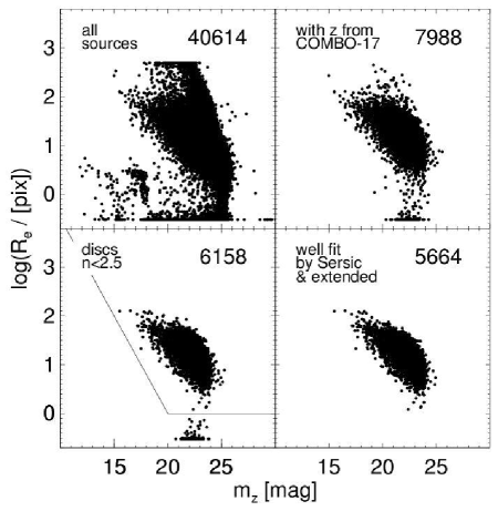
Figure 1.— The disk sample definition in the apparent magnitude–size plane (apparent effective radius: $R_{e}^{\textrm{\tiny{app}}}$, apparent $z$-band magnitude: $m_{z}$). Top left: all galaxies detected in the GEMS tiles. Top right: galaxies with COMBO-17 redshifts. Bottom left: disk galaxies with Sérsic index $n<2.5$. Bottom right: disk galaxies with reliable galfit fits (see text for details on selection criteria). In each panel, we give the total number of galaxies in the upper right.

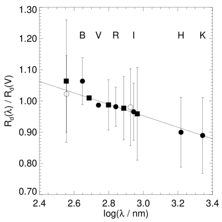
Figure 2.— The average ratio of the disk scale length $R_{d}\left(\lambda\right)$ measured in various bands ($B$, $V$, $R$, $I$, $H$, $K$) over $R_{d}\left(V\right)$ measured in the $V$-band for the de Jong (1996) data as a function of corresponding wavelength $\lambda$ (solid dots). The solid line marks a linear fit $f$, which is constrained to $f\left(2.74\right)=1$ at the $V$-band (not strictly requiring coincidence with the data point at the $V$-band). Over the redshift range sampled by the GEMS data the size corrections as inferred from this plot are of order $\pm 3\%$. Errors indicate the dispersion of the distribution of $R_{d}\left(\lambda\right)/R_{d}\left(V\right)$; they do not represent errors of the mean values plotted here. Solid boxes mark data points from the SDSS DR2 data set (see $\S$ 2.5 for details). Since there is no direct measurement in the $V$-band available for these objects, the data points are simultaneously fit minimizing the total offset between SDSS and de Jong values using the $g_{AB}$-band as the reference filter. Open symbols represent measurements from the GEMS survey where in a certain redshift bin one of the filters matched the rest-frame $V$-band.

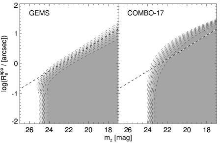
Figure 3.— The GEMS (left panel) and the COMBO-17 (right panel) detection probabilites as a function of apparent $z$-band magnitude $m_{z}$ and apparent half-light radius $R_{e}^{\textrm{\tiny{app}}}$. The contours indicate different detection probability levels (from light to dark shades of grey: 10%, 20%, 30%,… 90%). For comparison, in both plots a line of constant apparent surface brightness $\mu_{z}^{\textrm{\tiny{app}}}=24$ mag arcsec^-2 is shown.

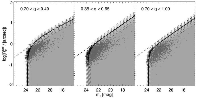
Figure 4.— The combined GEMS / COMBO-17 completeness (dashed contours indicating 10%, 20%, 30%,… 90%) in the $R_{e}^{\textrm{\tiny{app}}}$-$m_{z}$-plane. The solid contour shows the 50% completeness limit. Dots and pluses indicate disk galaxies with a combined GEMS detection / COMBO-17 redshift estimation probability $p>50\%$ and $p<50\%$, respectively. The panels show the completeness contours and data points for three different axis ratio ranges, indicated in the top of each plot. The diagonal line indicates a constant apparent surface brightness $\mu_{z}^{\textrm{\tiny{app}}}=24$ mag arcsec^-2.

Figure 5.— The SDSS completness as a function of apparent surface brightness $\mu_{50,r}$. The dots indicate the actual surface brightness values as given in Blanton et al. (2004). The solid line represents our analytical fit to that relation.

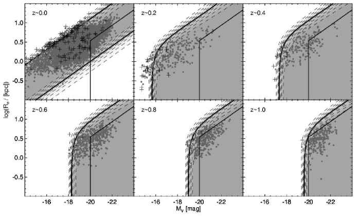
Figure 6.— The completeness as a function of redshift in the absolute magnitude–size plane. The same completeness contours and objects from the middle panel of Fig. 4 are plotted. The $z\sim 0$ bin shows the SDSS data. The contours were computed for the central redshift of each bin as indicated in the top left of each panel. Galaxies with low detection probability are found along the absolute magnitude limit, but not at bright magnitudes and faint surface brightnesses. The box in each panel encloses a selection with $\mu_{V}^{\textrm{\tiny{lim}}}=22$ mag arcsec^-2 and $M_{V}^{\textrm{\tiny{lim}}}=-20$. This plot shows that the GEMS data ($0.2<z<1.0$) are not limited in surface brightness. Galaxies are observed in regions where the completeness contours indicate detection probabilities $p<5\%$. This is a result of the finite width of the redshift bins (see $\S$ 4.1 and Fig. 7 for further explanations).

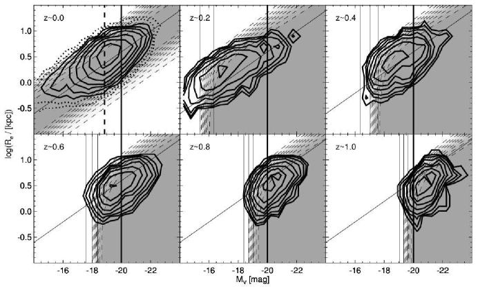
Figure 7.— The magnitude–size relation for six different redshift bins. The solid contours indicate 11 levels of fractional number of objects per unit area. To obtain the contours the density field was normalised by the total number of objects being plotted in each redshift bin and the following scaling was used: $\left(\exp\left(x/2\right)-1\right)\times 0.0005$, with $x=[1,2,...,11]$. The dotted contours are only shown for the lowest redshift bin ($z\sim 0$; SDSS data) for being too noisy in the other bins. The grey-scale contours mark the same completeness levels as shown in Fig. 6. The thin vertical lines in each panel symbolise an apparent magnitude $m_{z}=24$ converted to the rest-frame at three different redshifts corresponding to the center, low and high end of each redshift bin. This illustrates why apparently so many galaxies especially in the low redshift bin were detected at completeness values close to zero. The diagonal line in each panel corresponds to the average surface brightness $\mu_{V}=20.84$ mag arcsec^-2 in the lowest redshift bin. The thick vertical line represents the lower magnitude limit ($M_{V}=-20$), below which we exclude galaxies from the analysis. The thick dashed line shows the magnitude limit of the highest redshift SDSS data; at fainter magnitudes the VAGC data become incomplete.

Figure 8.— Histograms of the absolute rest-frame surface brightness as a function of redshift ($z\sim 0$ from SDSS; $0.2<z<1.0$ from GEMS). The histograms include weighting of individual objects according to their completeness (y-axis peak normalized). Only objects with a completeness exceeding 50% and with $M_{V}<-20$ were included in order to minimize the impact of selection effects. The black circle marks the estimated mean value $\left\langle\mu_{V}\left(z\right)\right\rangle$ for each redshift bin. In each redshift bin with $z>0.0$ we overplotted as open circles values of $\left\langle\mu_{V}\left(z\right)\right\rangle$ of all lower redshift bins to visualize the evolution in surface brightness. The vertical line in each panel indicates the Freeman (1970) surface brightness converted to the $V$-band (conversion given in Fukugita et al., 1995). The numbers in the top left of each panel shows the number of sources used in each panel (not including weighting).

Figure 9.— Evolution of the average absolute surface brightness $\left\langle\mu_{V}\left(z\right)\right\rangle$. Solid dots show the GEMS data for the individual redshift bins; the box symbol at $z\sim 0.05$ indicates the SDSS data point. The error bars mark $2\sigma$ statistical errors. The horizontal line at $\mu_{V}=21.05$ represents the Freeman (1970) surface brightness converted to the $V$-band. The solid and dotted lines mark a linear fit to all data points plus the $1\sigma$ confidence limits, respectively.

Figure 10.— The stellar mass–size relation for six different redshift bins ($z\sim 0$ from SDSS; $0.2<z<1.0$ from GEMS). The contours indicate levels of the same fractional number of objects per unit area as in Fig. 7. The vertical line in each panel marks $\log\left(\mathcal{M}/\mathcal{M}_{\odot}\right)=10$, which corresponds to the limiting stellar mass $\log\mathcal{M}^{\lim}$ applied to each redshift bin. The diagonal line in each panel corresponds to the average surface mass density measured from all redshift bins $\left\langle\log\Sigma_{\mathcal{M}}\left(z=1\right)\right\rangle=8.50$.

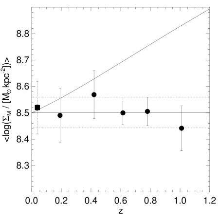
Figure 11.— Evolution of the average stellar surface mass density $\left\langle\log\Sigma_{\mathcal{M}}\left(z\right)\right\rangle$. Solid dots show the GEMS data for the individual redshift bins; the box symbol at $z\sim 0.05$ indicates the SDSS data point. The solid error bars indicate the $2\sigma$ statistical errors; the dotted error bar for the SDSS data point marks the $2\sigma$ systematic error resulting from the conversion of a mass-to-light ratio. The horizontal solid and dotted lines at $\left\langle\log\Sigma_{\mathcal{M}}\left(z\right)\right\rangle=8.50\pm 0.03$ represent a linear fit to the data with a constant slope of zero and the $1\sigma$ confidence limits, respectively. The diagonal line indicates the evolution as obtained from Mo et al. (1998).

Figure 12.— Histograms of the stellar surface mass density as a function of redshift ($z\sim 0$ from SDSS; $0.2<z<1.0$ from GEMS). The histograms include weighting of individual objects according to their completeness (y-axis peak normalized). Only objects with a completeness exceeding 50% and with $\log\left(\mathcal{M}/\mathcal{M}_{\odot}\right)>\log\mathcal{M}^{\lim}=10$ were included in order to minimize the impact of selection effects. The black circle marks the estimated mean value $\left\langle\log\Sigma_{\mathcal{M}}\left(z\right)\right\rangle$ for each redshift bin. In each redshift bin with $z>0.0$ we overplotted as open circles values of $\left\langle\log\Sigma_{\mathcal{M}}\left(z\right)\right\rangle$ of all lower redshift bins to visualize the evolution in surface mass density. The numbers in the top left of each panel shows the number of sources used in each panel (not including weighting).

Figure 13.— Comparison of the evolution of the average absolute central $B$-band surface brightness $\left\langle\mu_{0,B}\left(z\right)\right\rangle$ with the literature. Solid dots show the GEMS data for the individual redshift bins; the box symbol at $z\sim 0.05$ indicates the SDSS data point. The error bars mark $2\sigma$ statistical errors. The horizontal line at $\mu_{0,B}=21.65$ represents the Freeman (1970) surface brightness. The solid and dotted lines mark a linear fit to all data points (including the SDSS value) plus the $1\sigma$ confidence limits, respectively. a) Comparison with Simard et al. (1999, star symbols). b) Reproducing the Ravindranath et al. (2004) analysis. Triangles show values obtained from the GEMS data using the selection in limiting surface brightness and absolute magnitude as chosen by Ravindranath et al. (2004). The open symbols indicate the impact of a population of high surface brightness galaxies at the highest redshift bin using the definition of Ravindranath et al. (open triangle, just barely visible above the filled triangle) and the definition by Simard et al. (open star). Especially when using the latter definition, the GEMS data with the Ravindranath et al. selection are consistent with no surface brightness evolution.

Figure C1.— The average surface brightness $\left\langle\mu_{V}\left(z\right)\right\rangle$ (left panel) and the average surface mass density $\left\langle\log\Sigma_{\mathcal{M}}\left(z\right)\right\rangle$ (right panel) for the different redshift bins as a function of the adopted cut-off detection probability $p_{\lim}$. Horizontal dotted lines mark the means of each redshift bin. In both panels an absolute limiting magnitude $M_{V}^{\lim}=-20$ was applied.

Figure C2.— The average surface brightness $\left\langle\mu_{V}\left(z\right)\right\rangle$ (left panel) and the average surface mass density $\left\langle\log\Sigma_{\mathcal{M}}\left(z\right)\right\rangle$ (right panel) for the different redshift bins as a function of the adopted surface brightness limit $\mu_{V}^{\lim}$. Horizontal dotted lines mark the means of each redshift bin. The values at $\mu_{V}^{\lim}=24$ are plotted to demonstrate the results in the case were no fixed surface brightness limit ($\mu_{V}^{\lim}=\infty$) is chosen. In both panels an absolute limiting magnitude $M_{V}^{\lim}=-20$ and a detection probability cut $p_{\lim}=0.5$ was applied. The vertical lines correspond to the 50% completeness limiting surface brightness for an axis ratio $q=0.5$ at the indicated redshift.

Figure C3.— The average surface brightness $\left\langle\mu_{V}\left(z\right)\right\rangle$ (left panel) and the average surface mass density $\left\langle\log\Sigma_{\mathcal{M}}\left(z\right)\right\rangle$ (right panel) for the different redshift bins as a function of the adopted absolute magnitude limit $M_{V}^{\lim}$ or the limiting stellar mass $\log\mathcal{M}^{\lim}$ (left and right panel, respectively). Horizontal dotted lines mark the means of each redshift bin. The values at $M_{V}^{\lim}=-18$ (left) and $\log\mathcal{M}^{\lim}=9$ (right) are plotted to demonstrate the results if no fixed absolute magnitude limit ($M_{V}^{\lim}=-\infty$) or stellar mass limit ($\log\mathcal{M}^{\lim}=-\infty$) is chosen. In both panels a detection probability cut $p_{\lim}=0.5$ was applied. The vertical lines in the left panel correspond to the 50% completeness limiting absolute magnitude at the indicated redshift.

References

- Abazajian et al. (2004) Abazajian, et al., 2004, AJ, 128, 502
- Andredakis et al. (1995) Andredakis, Y. C., Peletier, R. F., & Balcells, M., 1995, MNRAS, 275, 874
- Bell & de Jong (2001) Bell, E. F., & de Jong, R. S., 2001, ApJ, 550, 212
- Bell et al. (2004) Bell, E. F., McIntosh, D. H., Barden, M., Wolf, C., Caldwell J. A. R., Rix, H., Beckwith, S. V. W., Borch, A., Häußler B., Jahnke, K., Jogee, S., Meisenheimer, K., Peng, C., Sanchez S. F., Somerville, R. S., & Wisotzki, L., 2004, ApJ, 600, L11
- Bell et al. (2003) Bell, E. F., McIntosh, D. H., Katz, N., & Weinberg, M. D., 2003, ApJS, 149, 289
- Bell et al. (2005) Bell E. F., Papovich C., Wolf C., Le Floc’h E., Caldwell J. A. R., Barden M., Egami E., McIntosh D. H., Meisenheimer K., Perez-Gonzalez P. G. P., Rieke G. H., Rieke M. J., Rigby J. R., & Rix H.-W., 2005
- Bertin & Arnouts (1996) Bertin, E., & Arnouts, S., 1996, A&AS, 117, 393
- Blanton et al. (2003) Blanton M. R., Brinkmann J., Csabai I., Doi M., Eisenstein D., Fukugita M., Gunn J. E., Hogg D. W., Schlegel D. J., 2003, AJ, 125, 2348
- Blanton et al. (2004) Blanton M. R., Schlegel D. J., Strauss M. A., Brinkmann J., Finkbeiner D., Fukugita M., Gunn J. E., Hogg D. W., Ivezic Z., Knapp G. R., Lupton R. H., Munn J. A., Schneider D. P., Tegmark M., Zehavi I., 2004, ApJ submitted
- Böhm et al. (2004) Böhm A., Ziegler B. L., Saglia R. P., Bender R., Fricke K. J., Gabasch A., Heidt J., Mehlert D., Noll S., & Seitz S., 2004, A&A, 420, 97
- Boissier & Prantzos (1999) Boissier, S., & Prantzos, N., 1999, MNRAS, 307, 857
- Borch (2004) Borch, A., 2004, Ph.D. Thesis, University of Heidelberg
- Bouwens & Silk (2002) Bouwens, R., & Silk, J., 2002, ApJ, 568, 522
- Bullock et al. (2001) Bullock, J. S., Dekel, A., Kolatt, T. S., Kravtsov, A. V., Klypin A. A., Porciani, C., & Primack, J. R., 2001, ApJ, 555, 240
- Bullock et al. (2001) Bullock, J. S., Kolatt, T. S., Sigad, Y., Somerville, R. S., Kravtsov A. V., Klypin, A. A., Primack, J. R., & Dekel, A., 2001, MNRAS, 321, 559
- Burstein et al. (1997a) Burstein, D., Bender, R., Faber, S., & Nolthenius, R., 1997a, AJ, 114, 1365
- Chiappini et al. (1997) Chiappini, C., Matteucci, F., & Gratton, R., 1997, ApJ, 477, 765
- de Jong (1996) de Jong R. S., 1996, A&AS, 118, 557
- D’Onghia & Burkert (2004) D’Onghia, E., & Burkert, A., 2004, ApJ, 612, L13
- Drory et al. (2004) Drory, N., Bender, R., & Hopp, U., 2004, ApJ, 616, L103
- Fall & Efstathiou (1980) Fall, S. M., & Efstathiou, G., 1980, MNRAS, 193, 189
- Ferguson & Johnson (2001) Ferguson, A. M. N., & Johnson, R. A., 2001, ApJ, 559, L13
- Flores et al. (1999) Flores H., Hammer F., Thuan T. X., Césarsky C., Desert F. X., Omont A., Lilly S. J., Eales S., Crampton D., & Le Fèvre O., 1999, ApJ, 517, 148
- Freeman (1970) Freeman, K. C., 1970, ApJ, 160, 811
- Fukugita et al. (1995) Fukugita, M., Shimasaku, K., & Ichikawa, T., 1995, PASP, 107, 945
- Giavalisco et al. (2004) Giavalisco, M., Ferguson, H. C., Koekemoer, A. M., Dickinson, M., Alexander, D. M., Bauer, F. E., Bergeron, J., Biagetti, C., Brandt W. N., Casertano, S., Cesarsky, C., Chatzichristou, E., Conselice C., Cristiani, S., Da Costa, L., & et al., 2004, ApJ, 600, L93
- Hammer et al. (2005) Hammer F., Flores H., Elbaz D., Zheng X. Z., Liang Y. C., & Cesarsky C., 2005
- Jahnke et al. (2004) Jahnke, K., Sánchez, S. F., Wisotzki, L., Barden, M., Beckwith, S. V. W., Bell, E. F., Borch, A., Caldwell, J. A. R., Häussler, B., Heymans, C., Jogee, S., McIntosh, D. H., Meisenheimer, K., Peng, C. Y., Rix, H.-W., Somerville, R. S., & Wolf, C., 2004, ApJ, 614, 568
- Kauffmann et al. (2003a) Kauffmann, G., Heckman, T. M., White, S. D. M., Charlot, S., Tremonti, C., Brinchmann, J., Bruzual, G., Peng, E. W., Seibert, M., Bernardi, M., Blanton, M., Brinkmann, J., Castander, F., Csábai, I., Fukugita, M., Ivezic, Z., et al., 2003a, MNRAS, 341, 33
- Kauffmann et al. (2003b) Kauffmann, G., Heckman, T. M., White, S. D. M., Charlot, S., Tremonti, C., Peng, E. W., Seibert, M., Brinkmann, J., Nichol, R. C., SubbaRao, M., & York, D., 2003b, MNRAS, 341, 54
- Kroupa et al. (1993) Kroupa, P., Tout, C. A., Gilmore, G., 1993, MNRAS, 262, 545
- Labbé et al. (2003) Labbé, I., Rudnick, G., Franx, M., Daddi, E., van Dokkum, P. G., Förster Schreiber, N. M., Kuijken, K., Moorwood, A., Rix, H., Röttgering, H., Trujillo, I., van der Wel, A., van der Werf, P., & van Starkenburg, L., 2003, ApJ, 591, L95
- Lilly et al. (1998) Lilly, S., Schade, D., Ellis, R., Le Fèvre, O., Brinchmann, J., Tresse, L., Abraham, R., Hammer, F., Crampton, D., Colless, M., Glazebrook, K., Mallen-Ornelas, G., & Broadhurst, T., 1998, ApJ, 500, 75+
- Maller et al. (2002) Maller, A. H., Dekel, A., & Somerville, R., 2002, MNRAS, 329, 423
- Mo et al. (1998) Mo, H. J., Mao, S., & White, S. D. M., 1998, MNRAS, 295, 319
- Navarro et al. (1997) Navarro, J. F., Frenk, C. S., & White, S. D. M., 1997, ApJ, 490, 493
- Navarro & Steinmetz (2000) Navarro, J. F., & Steinmetz, M., 2000, ApJ, 538, 477
- Navarro & White (1994) Navarro, J. F., & White, S. D. M., 1994, MNRAS, 267, 401
- Peebles (1969) Peebles, P. J. E., 1969, ApJ, 155, 393
- Peng et al. (2002) Peng, C. Y., Ho, L. C., Impey, C. D., & Rix, H., 2002, AJ, 124, 266
- Ravindranath et al. (2004) Ravindranath, S., Ferguson, H. C., Conselice, C., Giavalisco, M., Dickinson, M., Chatzichristou, E., de Mello, D., Fall, S. M., Gardner, J. P., Grogin, N. A., Hornschemeier, A., Jogee, S., Koekemoer, A., Kretchmer, C., Livio, M., et al., 2004, ApJ, 604, L9
- Rix et al. (2004) Rix, H., Barden, M., Beckwith, S. V. W., Bell, E. F., Borch, A., Caldwell, J. A. R., Häußler, B., Jahnke, K., Jogee, S., McIntosh, D. H., Meisenheimer, K., Peng, C. Y., Sanchez, S. F., Somerville, R. S., Wisotzki, L., & Wolf, C., 2004, ApJS, 152, 163
- Rocha-Pinto et al. (2000) Rocha-Pinto, H. J., Scalo, J., Maciel, W. J., & Flynn, C., 2000, A&A, 358, 869
- Sérsic (1968) Sérsic, J. L., 1968, Atlas de Galaxias Australes. Córdoba, Obs. Astron., Univ. Nac. Córdoba, 1968
- Shen et al. (2003) Shen, S., Mo, H. J., White, S. D. M., Blanton, M. R., Kauffmann, G., Voges, W., Brinkmann, J., & Csabai, I., 2003, MNRAS, 343, 978
- Sheth & Tormen (2004) Sheth, R. K., & Tormen, G., 2004, MNRAS, 349, 1464
- Simard et al. (1999) Simard, L., Koo, D. C., Faber, S. M., Sarajedini, V. L., Vogt, N. P., Phillips, A. C., Gebhardt, K., Illingworth, G. D., & Wu, K. L., 1999, ApJ, 519, 563
- Simard et al. (2002) Simard, L., Willmer, C. N. A., Vogt, N. P., Sarajedini, V. L., Phillips, A. C., Weiner, B. J., Koo, D. C., Im, M., Illingworth G. D., & Faber, S. M., 2002, ApJS, 142, 1
- Sommer-Larsen & Dolgov (2001) Sommer-Larsen, J., & Dolgov, A., 2001, ApJ, 551, 608
- Sommer-Larsen et al. (1999) Sommer-Larsen, J., Gelato, S., & Vedel, H., 1999, ApJ, 519, 501
- Spergel et al. (2003) Spergel, D. N., Verde, L., Peiris, H. V., Komatsu, E., Nolta, M. R., Bennett, C. L., Halpern, M., Hinshaw, G., Jarosik, N., Kogut, A., Limon, M., Meyer, S. S., Page, L., Tucker, G. S., Weiland, J. L., Wollack, E., & Wright, E. L., 2003, ApJS, 148, 175
- Steinmetz & Navarro (2002) Steinmetz, M., & Navarro, J. F., 2002, New Astronomy, 7, 155
- Thacker & Couchman (2001) Thacker, R. J., & Couchman, H. M. P., 2001, ApJ, 555, L17
- Trujillo & Aguerri (2004) Trujillo, I., & Aguerri, J. A. L., 2004, MNRAS, 355, 82
- Trujillo et al. (2004) Trujillo, I., Rudnick, G., Rix, H., Labbé, I., Franx, M., Daddi, E., van Dokkum, P. G., Förster Schreiber, N. M., Kuijken K., Moorwood, A., Röttgering, H., van de Wel, A., van der Werf P., & van Starkenburg, L., 2004, ApJ, 604, 521
- Vitvitska et al. (2002) Vitvitska, M., Klypin, A. A., Kravtsov, A. V., Wechsler, R. H., Primack, J. R., & Bullock, J. S., 2002, ApJ, 581, 799
- Vogt et al. (1996) Vogt N. P., Forbes D. A., Phillips A. C., Gronwall C., Faber S. M., Illingworth G. D., & Koo D. C., 1996, ApJ, 465, L15
- Weil et al. (1998) Weil, M. L., Eke, V. R., & Efstathiou, G., 1998, MNRAS, 300, 773
- Wolf et al. (2004) Wolf, C., Meisenheimer, K., Kleinheinrich, M., Borch, A., Dye, S., Gray, M., Wisotzki, L., Bell, E. F., Rix, H.-W., Cimatti, A., Hasinger, G., & Szokoly, G., 2004, A&A, 421, 913
- Wolf et al. (2003) Wolf, C., Meisenheimer, K., Rix, H.-W., Borch, A., Dye, S., & Kleinheinrich, M., 2003, A&A, 401, 73