The luminosity function of Ly$\alpha$ emitters at $2.3<z<4.6$ from integral-field spectroscopy

Abstract

We have used VIsible MultiObject Spectrograph Integral-Field Unit (VIMOS-IFU) observations centred on a radio galaxy at $z=2.9$ to search for Ly$\alpha$ emitters within a comoving volume of $\sim 10^{4}$ Mpc³. We find 14 Ly$\alpha$ emitters with flux $>1.4\times 10^{-20}$ W m^-2, yielding a comoving space density of $0.0018^{+0.0006}_{-0.0005}$ Mpc^-3. We fit a Schechter luminosity function which agrees well with previous studies both at similar redshift ($z\sim 3.4$) and higher redshift ($z\sim 5.7$). We therefore find no evidence for evolution in the properties of Ly$\alpha$ emitters between $3<z<6$, although our sample is small. By summing the star-formation rates of the individual Ly$\alpha$ emitters we find a total cosmic star-formation rate density of $\rho_{SFR}=6.7\pm 0.5\times 10^{-3}$ M_⊙yr^-1Mpc^-3. Integrating over the luminosity function for the combined Ly$\alpha$ surveys at $z\sim 3.4$ and accounting for the difference in obscuration between the Ly$\alpha$ line and the UV-continuum yields an estimate of $\rho_{SFR}\sim 2.2\times 10^{-2}$ M_⊙yr^-1Mpc^-3, in line with previous multi-colour and narrow-band surveys of high-redshift star-forming galaxies.

The detection of high-redshift emission-line galaxies in our volumetric search shows that the unique capabilities of wide-field integral-field spectroscopy are well suited in searching for high-redshift galaxies in a relatively unbiased manner.

1 INTRODUCTION

One of the most important questions in cosmology is how the Universe evolved into what we see today. It is believed that structure forms from the initial density perturbations in the dark matter distribution which collapse under gravitational instability (Eggen et al., 1962; Sandage et al., 1970; Peebles, 1971; Press & Schechter, 1974; White & Rees, 1978). The gravitational attraction of the dark matter overdensity causes gas to accumulate and cool, thus enabling star formation (White & Rees, 1978). Hierarchical models of galaxy formation postulate that these sub-galactic clumps subsequently merge to form larger galaxies. Studying star-forming galaxies as a function of both luminosity (or star-formation rate) and redshift is therefore essential to obtain insight into the formation history of galaxies.

As galaxies form and evolve they also influence their environment. The most obvious way in which this happens is that they are able to ionise the gas surrounding them. Observations of distant quasi stellar objects (QSOs) exhibit absorption shortward of the Ly$\alpha$ line (Gunn & Peterson, 1965), which indicates that the reionisation of the Universe was not yet complete at $z>6$ (e.g. Becker et al., 2001; Djorgovski et al., 2001). The vital question remains: which objects are responsible for this process? Again analysing the properties of primeval galaxies can provide an answer as the radiation emitted by the young OB-stars could be energetic enough to ionise the intergalactic medium (see e.g. Madau et al., 1999).

To detect primeval galaxies and determine the cosmic star-formation rate density, two different types of object are often targeted. One comprises the Lyman Break Galaxies, which are star-forming galaxies characterised by a strong break in their spectrum shortward of the Lyman limit at 912Å and the hydrogen Ly$\alpha$ line at 1216Å. The other type is the focus of this paper: the Ly$\alpha$ emitters, identified by their prominent emission in the Ly$\alpha$ line. Lyman Break Galaxies have been discovered in huge numbers over the past decade using multi-colour surveys (e.g. Steidel et al., 1999). Using this technique several surveys, probing different ranges in redshift, indicate a roughly constant star-formation rate density between $1<z<5$ (Connolly et al., 1997; Madau et al., 1998; Steidel et al., 1999; Iwata et al., 2003). However, at $z>6$ the star-formation rate density seems to decline (Stanway et al., 2003; Bunker et al., 2004) possibly indicating that the source of reionisation may not be the star-forming galaxies we see at $z<6$. Searches for Ly$\alpha$ emitters are complementary in this goal as these surveys can probe galaxies with relatively very weak continuum emission - undetected by the Lyman Break technique.

Several techniques have been used to observe high-redshift Ly$\alpha$ emitters: (i) slitless spectroscopy (e.g. Koo & Kron, 1980), (ii) slit-spectroscopy (e.g. Lowenthal et al., 1990; Thompson et al., 1992), and (iii) narrow-band imaging (e.g. Hu et al., 1997; Cowie & Hu, 1998). Each method has its pros and cons. Slitless spectroscopy allows a large volume to be probed, but needs very long integration times to achieve an acceptable flux limit. Slit-spectroscopy can achieve a good flux limit with shorter integration times but unfortunately the surveyed volume is often very small and multi-colour imaging observations are usually needed to preselect candidates. Narrow-band imaging compares broad-band images to images taken with a filter of very narrow bandwidth (e.g. $\Delta\lambda\sim 60$Å). Objects that are significantly brighter in the narrow-band image are likely to have a strong emission line at the observed wavelength of the narrow-band filter. This way large areas can be searched for Ly$\alpha$ emitters. This type of survey has been the most successful in detecting Ly$\alpha$ emitters since the late 1990s when the sensitivity of the surveys increased considerably due to the onset of 8-metre and 10-metre class telescopes (e.g. Hu et al., 1997; Cowie & Hu, 1998).

With this leap in collecting area, detection of Ly$\alpha$ emitters through narrow-band imaging has frequently been used to determine the cosmic star-formation rate density from $z\approx 3-7$ (e.g. Kudritzki et al., 2000; Fujita et al., 2003; Kodaira et al., 2003). Nevertheless narrow-band imaging suffers from one major drawback: due to the small FWHM of the narrow-band filter, the surveys sample a very narrow redshift range, and thus a shallow volume. Hence it is impossible to use a single narrow-band survey to determine the Ly$\alpha$ density and luminosity function throughout a large redshift range.

In this paper we aim to improve upon these limitations by searching for Ly$\alpha$ emitters with integral-field spectroscopy. An Integral-Field Unit (IFU) samples an area on the sky where every pixel contains a spectrum. This then allows a volume of the Universe to be probed with just a single observation. Thus depending on the wavelength range probed we are able to study the comoving space density and properties of Ly$\alpha$ emitters over a large redshift range.

We have used the VIsible MultiObject Spectrograph Integral-Field Unit (VIMOS-IFU, LeFevre et al., 2003) on the Very Large Telescope to search for Ly$\alpha$ emitters within a volume of $\sim 10^{4}$ Mpc³. In section 2 we describe our observations and the data reduction and section 3 details the selection procedure used to find Ly$\alpha$ emitters in our data. The results are presented in section 4; section 5 discusses our findings and in section 6 we provide a summary of our conclusions. Throughout this paper we assume $\Omega_{\rm matter}=0.3$, $\Omega_{\Lambda}=0.7$, and $H_{0}=71$ km s^-1Mpc^-1, unless stated otherwise.

2 OBSERVATIONS AND DATA REDUCTION

All of our observations were made on the nights of 29 April 2003 to 2 May 2003 on the 8.2-metre Melipal telescope at the ESO Paranal Observatory in Chile. We used the VIMOS-IFU which consists of 6400 fibres coupled to microlenses. Each fibre produces a spectrum of a small region on the sky; these spectra can be integrated to construct a ‘broad-band’ image, as shown in Fig. 1. Our observations were made in low-resolution mode which corresponds to a resolution of $R\approx 250$. The spectral wavelength range was 3500Å $\rightarrow$ 7000Å with a dispersion of 5.35 Å per pixel. The spatial sampling of the fibres in our set-up was 0.67 arcsec per fibre, resulting in a square continuous field of view of $54\times 54$ arcsec² with the dead space between the fibres comprising less than 10% of the fibre to fibre distance. The field is split up into four quadrants, each connected with an EEV CCD detector consisting of 2048 x 4096 pixels.

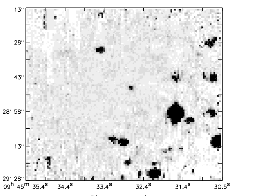
Figure 1: The two-dimensional image of our IFU field of view, integrated from 4050 Å to 6800 Å.

The observations were centred on MRC 0943-242, a powerful radio galaxy at $z=2.92$ ($\alpha=9^{h}45^{m}32.7^{s}$, $\delta=-24^{\circ}28^{\prime}49.7^{\prime\prime}$, J2000). The total exposure time was 9 hours, split into 18 exposures of 30 minutes. In order to minimise the effects of bad pixels and contamination by cosmic rays during data reduction, the consecutive exposures were offset by 10 arcsec in both right ascension and declination relative to the centre. During all four nights the seeing varied between 0.6 and 0.8 arcsec.

The data were reduced using the VIMOS Interactive Pipeline Graphical Interface (VIPGI, Scodeggio et al., 2004). First the standard routines for bias and flat-field correction are applied. Subsequently the individual spectra on the science frames are separated from each other. Each frame consists of 400 spectra, corresponding to one quadrant of the IFU. The layout of the IFU fibres in the instrument focal plane is used to calculate the position of the individual spectra on the CCD frame. When the spectra are located, the wavelength calibration is derived specifically for each fibre by identifying arc lamp lines taken with the same set-up. The variations in the transmission of the individual fibres are corrected for and a sky estimate is calculated by averaging the individual spectra. The sky spectrum is then subtracted from the individual spectra and cosmic rays are removed using a 3$\sigma$ clipping algorithm on the data. The spectra are flux calibrated using standard-star frames. To this end the instrument sensitivity function is derived by summing the spectra which contain flux from the standard star. This results in an accurate relative flux calibration. To obtain the absolute flux calibration, we use a long-slit spectrum of the central radio galaxy taken with the LRIS on the Keck Telescope. We measure the flux of the Ly$\alpha$ line by integrating the flux in the LRIS-spectrum and construct a spectrum of the same object with the VIMOS-IFU data by summing the fibres along the long-slit orientation. This allows us to bootstrap the spectrophotometry. Comparisons of spectra and V-band photometry of several objects in the field show that the final flux calibration is good to $\sim 20$ per cent. The effect of the dead space between the fibres on the error in the flux measurement is negligible as it is inherently small and has been even further reduced by the dithering of our single exposures.

The science frames are median combined to remove any remaining cosmic rays and a fringe correction is applied by median combining the fringe frames. The final data cube consists of 12100 combined spectra, as a result from our enlarged field of view due to the dithering of the individual exposures. These 12100 spectra correspond to a two-dimensional image of $110\times 110$ pixels with a field of view of $1.2^{\prime}\times 1.2^{\prime}$ (see Fig. 1).

3 DATA ANALYSIS

3.1 The sensitivity of the data

To determine the sensitivity of the data a wavelength range is selected where the flux calibration is good and the spectra are clear of skylines. At both ends of the spectra the flux calibration is poor, so we discard the regions at $3500$Å $<\lambda<4200$Å and $6800$Å $<\lambda<7000$Å. Between $\lambda=5500$Å and $\lambda=6550$Å three skylines dominate the spectra; this region is also omitted from the determination of the sensitivity function. In each spectrum we fit a polynomial to the usable wavelength range to facilitate calculation of the Root Mean Square (RMS) of the noise ($\sigma$). The fit is subtracted from the data and $\sigma$ is calculated. As the presence of actual features in the spectrum would alter the value of the noise, data points deviating more then $3\sigma$ from the fit are discarded. Subsequently the RMS of the noise is recalculated. This procedure results in a measurement of the overall RMS of the noise in each spectrum.

Visual inspection of random spectra with the continuum fit and noise estimate confirm that the measurements are accurate. The method does not work well in fibres where there are bright objects, e.g. stars or nearby galaxies, due to the large number of emission and/or absorption lines in the spectrum. However, to search for distant Ly$\alpha$ emitters we want to avoid those regions of the sky with bright nearby objects. Therefore the sensitivity determination described above is well suited to our needs as it yields an accurate value for the noise in spectra that do not sample luminous sources. To be able to exclude regions with bright objects the noise value in the corresponding fibres is set to zero. Inspection of the spectra of these objects reveals them to be nearby galaxies, stars, a QSO at $z=1.8$ (see , Jarvis, van Breukelen, & Wilman2005) and a galaxy at $z=0.62$, identified through its [OII] emission. In Fig. 2 the sensitivity function over the two-dimensional image is shown. Note that, especially in the smoothed image, the effects of dithering the exposures are evident. The noise varies from $\sigma=1.4\times 10^{-21}$ W m^-2pix^-1 to $6.2\times 10^{-21}$ W m^-2pix^-1 over the data cube.

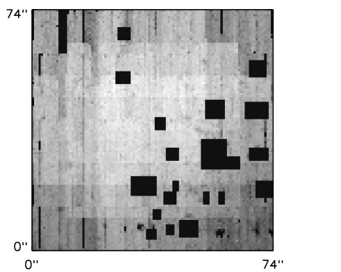
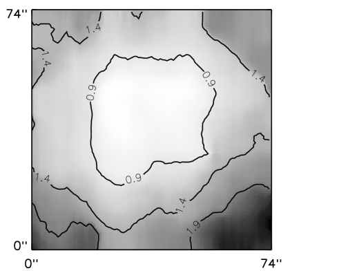
Figure 2: The sensitivity function over our field of view. The lighter regions correspond to better sensitivity. Top: pixel to pixel sensitivity function; regions with bright objects are set to zero. Bottom: smoothed sensitivity function to show the effects of the dithered single exposures. The $5\sigma$ sensitivity varies between $6.8\times 10^{-21}$ W m^-2pix^-1 (white) to $3.1\times 10^{-20}$ W m^-2pix^-1 (black). The contours shown are at 0.9, 1.4, and $1.9\times^{-20}$ W m^-2pix^-1.

Table 1: Observed Ly$\alpha$ emitters with their observational properties. The typical errors on the quoted positions are 0.3” and reflect the size of the IFU-fibres. The wavelength, flux, and their errors are calculated by a repeated Gaussian fit to the emission lines as described in section 4.1. A star symbol ($*$) following the candidate number signifies an extended source (i.e. the emission line is spread over more than one IFU fibre). All luminosities $L_{\rm line}$ quoted assume that the line lies at the redshift $z$, given in column 6.

Nr.	RA (J2000)	Dec	$\lambda$	Fline	z	Lline
	h   m   s	∘    ′    ′′	Å	$10^{-20}$ W m-2		$10^{35}$ W
532*	9:45:30.64	-24:28:26.9	5752$\pm$1	3.0$\pm$0.7	3.7315$\pm$0.0008	4.1$\pm$0.9
1315*	9:45:30.95	-24:28:18.2	5140$\pm$1	6.7$\pm$1.8	3.2281$\pm$0.0008	6.4$\pm$1.7
1702*	9:45:31.13	-24:28:53.7	5699$\pm$1	2.7$\pm$0.8	3.6879$\pm$0.0008	3.6$\pm$1.1
2919	9:45:31.62	-24:28:49.0	5437$\pm$1	1.4$\pm$0.4	3.4724$\pm$0.0008	1.6$\pm$0.5
3210*	9:45:31.76	-24:29:15.1	4676$\pm$1	5.5$\pm$1.0	2.8464$\pm$0.0008	3.9$\pm$0.7
3510	9:45:31.85	-24:28:21.5	6601$\pm$1	2.1$\pm$0.5	4.4299$\pm$0.0008	4.3$\pm$1.0
5644*	9:45:32.74	-24:29:05.8	4766$\pm$1	7.3$\pm$1.4	2.9205$\pm$0.0008	5.5$\pm$1.1
6164	9:45:32.96	-24:29:25.9	4341$\pm$1	3.9$\pm$0.8	2.5709$\pm$0.0008	2.1$\pm$0.4
6537	9:45:33.10	-24:28:57.1	6619$\pm$1	1.5$\pm$0.3	4.4447$\pm$0.0008	3.1$\pm$0.6
8060	9:45:33.72	-24:29:08.4	4861$\pm$2	1.7$\pm$0.6	2.9986$\pm$0.0016	1.4$\pm$0.5
8599	9:45:33.95	-24:29:15.8	4280$\pm$1	1.8$\pm$0.5	2.5207$\pm$0.0008	0.9$\pm$0.3
8827	9:45:34.03	-24:29:10.5	4234$\pm$2	2.1$\pm$0.7	2.4829$\pm$0.0016	1.1$\pm$0.4
8893	9:45:34.03	-24:28:26.2	4611$\pm$1	2.3$\pm$0.5	2.7930$\pm$0.0008	1.5$\pm$0.3
10913	9:45:34.88	-24:29:13.1	4232$\pm$1	2.3$\pm$0.6	2.4812$\pm$0.0008	1.2$\pm$0.3

3.2 Selection of line emitters

With a dispersion of  5.35Å per pixel and a resolution of $R\approx 250$, the FWHM of the emission lines will generally be only about 3 pixels as we expect the typical Ly$\alpha$ emitter to have an unresolved Ly$\alpha$ line at this resolution. As the lines may well appear narrower due to the noise, we select peaks with a maximum value over $4\sigma$ above the previously determined fit to the continuum level and a 2-pixel integrated flux greater than $5\sigma$. Taking a lower limit than 4$\sigma$ for the peak value of the line leads to too much confusion with peaks in the noise; furthermore the detection completeness of the low-flux lines would be very low. The integrated 5$\sigma$ flux limit will result in the detection of emission lines with a lower limit to the flux varying over the whole field between 1.0$\times 10^{-20}$ W m^-2 and 4.4$\times 10^{-20}$ W m^-2 for an unresolved emission line, as derived from the sensitivity function. We only investigate the wavelength ranges $4050$Å $<\lambda<5520$Å, $5625$Å $<\lambda<5850$Å, $5950$Å $<\lambda<6130$Å, and $6550$Å $<\lambda<6800$Å to avoid skylines and distortion by bad flux calibration. After selecting all peaks in the spectra that satisfy the imposed criteria, the peaks that are clearly caused by bad pixels, poor flux calibration or other irregularities in the data are discarded. We verify the selection procedure by performing a number of tests. First, the same selection process is run again with a smoothed sensitivity function (see bottom Fig. 2) instead of the pixel-to-pixel values (top Fig. 2). In this way we check if any candidates are selected or rejected due to errors in the noise determination in individual fibres; we also run this test without fitting the continuum, to make sure there are no line candidates selected or discarded through an erroneous fit. The spectra of the remaining line candidates are then inspected by eye. To this point the RMS of the least noisy parts of the spectrum have been used to identify candidate line emitters. However, some parts of the spectrum are noisier, therefore the local RMS of the noise around the line candidate is determined to check if the peak value is still above 4$\sigma$. We then calculate the integrated flux over the two highest pixels to ensure that it is more than 5 times the RMS of the integrated local noise.
Bad pixels and cosmic rays affect the final image even in the data cube consisting of the combined frames. Moreover first order superpositions are not well removed during the data reduction nor are the reduced frames always clear of sky line residues. Therefore we construct two more data cubes, comprising 8 and 10 original exposures respectively, and calculate at what level the line should be detected if it is real. If the line is clearly present in one cube, but not in the other, it is likely to be an artefact seen in only one or a few original frames. Subsequently for each line candidate all the single exposures are visually inspected for artefacts. The final check is to see if the line could be the result of crosstalk between fibres, which is caused by overflowing of the light from a fibre into a neighbouring fibre on the CCD. These neighbouring fibres do not necessarily correspond to adjoining positions on the sky as there is a complicated mapping of fibres from the IFU-head onto the CCD. If a line candidate passes all these tests, it is declared to be a real emission line. After all of these consistency checks we find 15 emission-line galaxies.

4 RESULTS

4.1 Properties of the line emitters

Our IFU data facilitates examination of both the spectral and spatial properties of the 15 line emitters we have found. The spectra of the 14 candidate Ly$\alpha$ emitters are shown in Fig. 3. The other source is a narrow-line active galaxy which is discussed fully in Jarvis et al. (2005).

Figure 3: Spectra of the identified line emitters. The positions of the emission lines are denoted by an arrow. The regions that were excluded from our analysis are shaded; at these wavelengths skylines or bad flux calibration dominate the spectra. The redshifts all assume that the emission line is Ly$\alpha$ .

Figure 3: cont.

For each candidate Ly$\alpha$ emitter we measure the total flux of the emission line by integrating over the spectra of all fibres sampling the source. The flux of each emission line is measured by fitting a Gaussian profile to the emission line. To determine the uncertainty in the line profile, we recalculate our fit 1000 times, each time adding to the spectrum random noise with an RMS corresponding to the local noise in the spectrum at the position of the emission line. The flux and the wavelength of the line are taken to be the mean of the 1000 calculations. The standard deviations correspond to the $1\sigma$ uncertainties on the flux and wavelength. The results of these fits can be found in Table 1.

With broad-band images of this field, we derive the continuum level of the candidate line emitters by measuring (or placing a lower limit on) their broad-band magnitude. The sources are taken to be detected if the flux within the IFU-fibre aperture is larger than $2\sigma$ above the background level. The V-band image is shown in Fig. 4; the locations of the line-emitters are indicated by circles which reflect the errors on the positions as quoted in Table 1. To verify the correctness of the identification of line emitters with objects in the broad-band images we compare the coordinates of six bright objects that are easily visible in the IFU data cube as well as the broad-band image. The mean difference between the two positions for each object is $\sim 0.3"$ in RA. In declination however the error varies from $\sim 0.3"$ in the centre of the field to $\sim 1"$ at the edges, and we return to this point in section 4.2.

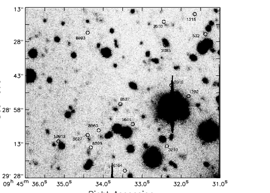
Figure 4: Keck V-band image of our field of view. The positions of the line emitters are marked by a circle the size of an IFU fibre. The accuracy in RA is $\sim 0.3"$; in Dec the error increases with distance from the centre from $0.3"$ to up to $\sim 1"$. This compromises the certainty of the identification of object 3510, 8599, and 8827.

4.2 Identification of the emission lines

It is possible not all our objects are actually Ly$\alpha$ emitters at high redshift, such that some may be low-redshift interlopers. Within our wavelength range any emission line is most likely to be either Ly$\alpha$ $\lambda 1216$, [OII] $\lambda 3727$, [OIII] $\lambda 5007$, or H$\alpha~{}\lambda 6563$. For each spectrum we inspect the plausibility of these four cases. The redshift of the object is calculated for each possible line and subsequently the redshifted wavelength of other emission lines are inspected by checking whether the signal at these positions is greater than $2\sigma$ above the local noise, which would indicate a possible detection. None of the spectra were found to exhibit any other lines under this criterion, which rules out the [OIII] $\lambda 5007$ and H$\alpha~{}\lambda 6563$ possibilities. However confusion with the [OII] $\lambda 3727$ line may still occur, since we would not expect to see other bright emission lines in our spectra if this is the observed line. The most distinguishing characteristic of the [OII] $\lambda 3727$ line is the fact that it is actually a doublet with lines at $\lambda=3726$Å and $\lambda=3728$Å; unfortunately due to our low resolution we cannot resolve this feature. We investigate how likely our lines are to be [OII] by calculating how many [OII] emitters we would expect to find in our volume according to Hogg et al. (1998), who carried out a survey at $z\sim 1$. For our observed wavelength range the [OII] emitters within our field of view would be at $0.087<z<0.825$, corresponding to a volume of 214 Mpc³ (here we use $\Omega_{\rm M}=0.3$, $\Omega_{\Lambda}=0$, and $H_{0}=100$ km s^-1Mpc^-1 to facilitate comparison with the [OII] survey of Hogg et al., 1998). Using the [OII] luminosity function combined with the sensitivity function derived from our data, we expect to detect 3 [OII] emitters in our volume. Indeed we have found one [OII] emitter at $z=0.62$ (see section 3.1) among the bright extended objects that we have excluded from our selection procedure. This galaxy could easily be identified as such by the clear presence of the 4000Å break in its continuum.

As derived from stellar synthesis models a Ly$\alpha$ line, originating from a young star-forming region, has a typical rest-frame equivalent width (EW₀) of 100-200Å, (Charlot & Fall, 1993). Surveys for Lyman Break Galaxies however often observe far lower equivalent widths for the Ly$\alpha$ line. At $z=3$ Shapley et al. (2003) find that only half of the Lyman Break Galaxies with observed Ly$\alpha$ emission show an EW₀ of $>20$Å and very few objects have EW${}_{0}>100$Å. Also at $z=6$ Lyman Break Galaxies usually show a detected EW₀ of $\sim 20-30$Å (Stanway et al., 2004). Nevertheless observations of Ly$\alpha$ emitters at high redshift show that many of these objects show a Ly$\alpha$ EW₀ of $>200$Å (e.g. Malhotra & Rhoads, 2002). Studies of [OII] emitters on the other hand show that their equivalent widths are considerably lower. For example Jansen et al. (2000) have carried out a survey of nearby field galaxies, which resulted in equivalent width measurements with a maximum of $\sim 80$ Å for [OII]. Measuring the EW of our emission lines thus provides a crucial test of whether the line is likely to be Ly$\alpha$ or [OII]. Using the flux of the lines and the (upper limit on) the continuum level, we calculate the (lower limit on) equivalent widths of the lines; these are shown in Table 2. For the objects detected in the band in which their emission line falls, we can use the broad-band images to check whether we can observe a spectral break due to hydrogen in the IGM. This is impossible for the objects with emission lines in the B-band as we have no bands at shorter wavelength. We have however one object (no. 1315) with an emission line in V-band that is also detected in that band; this object has $(B-V)>1.3$. Dickinson (1998) imposes a limit of $(B-V)>1.5$ to select Lyman Break Galaxies, which means that our B-band image is not deep enough to conclusively determine if we see a strong spectral break, although the lower limit to the object’s colour is close to the selection criterion. The broad-band identification for objects 3510, 8599, and 8827 are insecure due to their proximity to faint objects in the broad-band images in regions of the field where our astrometry becomes less secure ($\Delta\delta\sim 1$ arcsec). Therefore we have calculated their EWs assuming both no identification and an identification with the source found in close proximity in the broad-band image.

As shown in Table 2, all but two of our unknown emission lines would have rest-frame equivalent widths of several hundred Å if they were [OII]. The low-redshift survey for [OII]-emitters by Jansen et al. (2000) did not yield any [OII] emission lines with an EW₀ larger than 80Å. In the survey at redshift $z\sim 1$ by Hogg et al. (1998) the highest detected EW₀ of [OII] is still below 110Å. It is therefore highly improbable that any of our high equivalent width emission lines are [OII]. Nevertheless there are two emission lines, in objects 3510 and 6537, which could plausibly be [OII], as the lower limit on their EWs would be $\sim 119$Å and $\sim$ 84Å respectively which is high but not impossibly so. However it needs to be noted that this does not stem from a faint line flux, but from the I-band magnitude limit which is much brighter than those of the other broad-band images. This results in a lower EW limit. Moreover the objects show no continuum or any other features in their spectra, and it is therefore likely that these objects are Ly$\alpha$ emitters too. Thus for the remainder of this paper we will assume that all of our selected candidates are indeed Ly$\alpha$ emitters. The inferred redshift and line luminosities for our objects are shown in Table 1.

Table 2: The equivalent widths of the emission lines of our candidate Ly$\alpha$ emitters. All values are lower limits unless preceded by ’=’, which represents the actual EW instead of the lower limit. EW_obs is the observed equivalent width, EW_0,[OII] is rest-frame EW assuming the observed line is [OII] and EW_0,Lyα is the rest-frame EW if the line is Ly$\alpha$. Quoted errors are the result of the uncertainty in the measured flux, magnitude, and redshift. Objects 3510, 8599, and 8827 have an insecure identification in the broad-band images. For object 3510 this makes no difference for the calculation of the EW as the nearby source is not detected in I-band (in which wavelength range its emission line falls). For objects 8599 and 8827 the EW is shown for both the case where the nearby source is (1) unassociated and (2) associated with the line emission.

Nr.	EWobs	EW0,OII	EW0,Lyα
	$10^{2}$ Å	$10^{2}$ Å	$10^{2}$ Å
532	11$\pm$3	7$\pm$2	2.3$\pm$0.5
1315	= 13$\pm$5	= 9$\pm$4	= 3.0$\pm$1.2
1702	10$\pm$3	6$\pm$2	2.0$\pm$0.6
2919	7$\pm$2	5$\pm$1	1.7$\pm$0.5
3210	12$\pm$2	10$\pm$2	3.2$\pm$0.6
3510	2.1$\pm$0.5	1.2$\pm$0.3	0.39$\pm$0.09
5644	= 10$\pm$5	= 8$\pm$4	= 2.6$\pm$1.2
6164	16$\pm$3	14$\pm$3	4.6$\pm$0.9
6537	1.5$\pm$0.3	0.8$\pm$0.2	0.28$\pm$0.05
8060	7$\pm$3	5$\pm$2	1.8$\pm$0.6
85991	8$\pm$2	7$\pm$2	2.1$\pm$0.6
85992	= 2.9$\pm$0.6	= 2.5$\pm$0.5	= 0.8$\pm$0.2
88271	9$\pm$3	8$\pm$3	2.5$\pm$0.8
88272	= 1.9$\pm$0.3	= 1.7$\pm$0.3	= 0.56$\pm$0.09
8893	10$\pm$2	8$\pm$2	2.5$\pm$0.6
10913	10$\pm$3	8$\pm$2	2.8$\pm$0.7

5 DISCUSSION AND CONCLUSIONS

5.1 The Ly$\alpha$ emitter luminosity function

Figure 5: The number density of Ly$\alpha$ emitters plotted against the luminosity. The filled symbols mark surveys with an average redshift similar to ours (Cowie & Hu (1998): triangles, Kudritzki et al. (2000): circles) and the open symbols stand for surveys at redshift $z=5.7$ (Ajiki et al. (2003): squares, Hu et al. (2004): upside-down triangles). Overplotted are two Schechter luminosity functions: the solid line is the fit to all our data points and the dashed line is the fit to our two highest luminosity data points and those of the surveys at similar redshift with $L>5\times 10^{35}$ W (dashed horizontal line) to ensure completeness. The dotted horizontal lines mark the detection limits of the surveys; for Ajiki et al. (2003) this is the completeness limit.

Our field of view of 1.2’ $\times$ 1.2’ gives a solid angle of 1.5 square arcmin. However, for our high-redshift Ly$\alpha$ search we have omitted the regions which contain bright objects. Accounting for this reduction in area due to the bright sources, we are left with a solid angle of 1.36 square arcmin. If we assume we are only looking at Ly$\alpha$ emitters, our observed wavelength ranges (see section 3.2) correspond to redshift ranges of $2.33<z<3.54$, $3.63<z<3.81$, $3.89<z<4.04$, and $4.39<4.59$, which yield a total comoving volume of $7.8\times 10^{3}$ Mpc³.

The redshift range is large, thus the average flux limit over our field of view of $1.8\times 10^{-20}$ W m^-2 (see Fig. 2) corresponds to a luminosity limit which rises significantly throughout the depth of our volume. If we calculate the average luminosity limit over our field we find that it varies within the extremes of our redshift range from $8\times 10^{34}$ W at $z=2.3$, to $4\times 10^{35}$ W at $z=4.6$.

Due to the unique nature of our observations we are able to probe the Ly$\alpha$ luminosity function across a wide range in luminosity, albeit with a broad redshift bin. In Fig. 5 we show the Ly$\alpha$ luminosity function derived from our observations together with those of Kudritzki et al. (2000, hereafter Ku00) at $z\approx 3.1$, Cowie & Hu (1998, hereafter CH98) at $z=3.4$, and Ajiki et al. (2003, hereafter Aj03) and Hu et al. (2004, hereafter Hu04) at $z\approx 5.7$. We have determined the volume of each of the luminosity bins by calculating the volume within which a source of that luminosity can be observed with our flux limit, which varies over the field of view according to the sensitivity function derived in section 3.1. Fig. 5 shows that we probe down to much lower luminosities than the narrow-band surveys at $z>3$; this stems from the fact that at the lower redshift limit of our volume we have a significantly lower luminosity limit. The lack of high-luminosity sources in our volume is caused by the small size of the area surveyed.

To determine if our luminosity function differs from those found by the previous surveys at both similar redshift and higher redshift, we fit a Schechter function to the data:

$$\Phi(L)dL=\Phi^{*}\Big{(}\frac{L}{L^{*}}\Big{)}^{\alpha}e^{-L/L^{*}}d\Big{(}\frac{L}{L^{*}}\Big{)},$$

where $\Phi(L)$ is the comoving space density of sources per $\Delta\log{L_{\rm Ly\alpha}}$, $\Phi^{*}$ is the normalisation, $L^{*}$ is the characteristic break luminosity, and $\alpha$ is the slope of the luminosity function. As our binned data-points are few, we choose not to fit the Schechter function with three free parameters. Therefore we assume $\alpha=-1.60$: the slope of the Schechter function for $z\approx 3$ Lyman Break Galaxies (Steidel et al., 1999), which also fits well to the luminosity distribution of $z\approx 3$ Ly$\alpha$ emitters (Steidel et al., 2000). We determine the best fit by carrying out a least-squares minimisation using $L^{*}$ and $\Phi^{*}$ as free parameters. The best fit to our data is given by $L^{*}=5.0\pm 1.8\times 10^{35}$ W and $\Phi^{*}=0.0012\pm 0.0005$ Mpc^-3 (shown in Fig. 5 by the solid curve). To ensure completeness we also fit a line to a dataset comprising our two highest-luminosity points and the results from CH98 and Ku00 at $L>5\times 10^{35}$ W, which are at similar redshift. We then obtain $L^{*}=5.4\pm 1.7\times 10^{35}$ W and $\Phi^{*}=0.0022\pm 0.0012$ Mpc^-3, shown by the dashed curve in Fig. 5. The two fits therefore agree with each other within the uncertainties.

It appears that the results of the higher-redshift surveys are largely consistent with the lower-redshift Ly$\alpha$ luminosity function, although the lowest-luminosity results are hampered by incompleteness. AJ03 have inferred the same fact by comparing their luminosity function with the results of CH98. Hu04 also report that the properties of their $z=5.7$ sample shows the same properties as their sample at $z\approx 3$ (Hu et al., 1998). The inferred conclusion is that the luminosity function of Ly$\alpha$ emitters does not significantly change from $z\approx 3.4$ to $z=5.7$. Malhotra & Rhoads (2004) have considered the evolution of the Ly$\alpha$ luminosity function at even higher redshift, comparing samples at $z=5.7$ and $z=6.5$. They conclude the luminosity functions do not statistically deviate from each other, implying that the reionisation of the Universe must have been largely complete at $z=6.5$.

We can calculate how many high-luminosity sources we would expect to find according to our luminosity function. In this way we can check our earlier statement that we find none of these objects because our probed volume is too small. If we integrate the luminosity function from the edge of our highest luminosity bin to infinity over the volume probed by our survey, we find that we would expect to find only one object with a higher Ly$\alpha$ luminosity. The lack of high-luminosity sources in our survey is therefore within the Poisson error of our expectation and is not significant.

5.2 The star-formation rate

Figure 6: Star-formation rate densities as derived by various types of surveys. The result from this work derived from integrating over the luminosity function fit to our data alone is denoted by the star symbol. The different types of surveys are marked with different symbols: the open circles are H$\alpha$ searches, the open triangles are surveys aimed at oxygen emission lines, the filled triangles are multi-colour surveys, and the open squares are Ly$\alpha$ searches. All the SFR densities and their relevant references can be found in Table 3. The x-error bars reflect the redshift range of the surveys.

As the Ly$\alpha$ line is excited when interstellar gas is photoionised by the UV radiation of young and hot blue stars, the Ly$\alpha$ luminosity of a galaxy is directly related to its star-formation rate (SFR). We can derive this relation by using the case B recombination theory (Brocklehurst, 1971) to deduce the H$\alpha$ luminosity of a star-forming galaxy from its Ly$\alpha$ luminosity, and the equation found by Kennicutt (1998) to link in turn its star-formation rate to its H$\alpha$ luminosity. The formulae are respectively $L_{\rm Ly\alpha}=8.7L_{\rm H\alpha}$, and $SFR=7.9\times 10^{-35}L_{\rm H\alpha}$ M_⊙yr^-1, where $L_{\rm H\alpha}$ is the H$\alpha$ luminosity in Watts and continuous star formation is assumed with a Salpeter Initial Mass Function from $0.1-100$ M_⊙. Thus we get:

$$SFR=9.1\times 10^{-36}\Big{(}\frac{L_{\rm Ly\alpha}}{\rm W}\Big{)}\rm{~{}M_{\odot}yr}^{-1}.$$

Using this relation we estimate the star-formation rate for each of our objects. It is important to note that these star-formation rates are calculated under the assumption that the Ly$\alpha$ line is solely photoionised by hot stars and neglecting any extinction. The SFRs range from about 1 to 6 solar masses per year, with an average of $2.6\pm 1.6$ M_⊙yr^-1.

Summing the individual SFRs of our objects and dividing by their corresponding volume gives a comoving star-formation rate density of $\rho_{SFR}=0.0067\pm 0.0005$ M_⊙yr^-1Mpc^-3. Integrating over the luminosity function yields $\rho_{SFR}=0.008$ M_⊙yr^-1Mpc^-3 for $L^{*}=5.0\times 10^{35}$ W and $\Phi^{*}=0.0012$ Mpc^-3, which applies to our own dataset, and $\rho_{SFR}\approx 0.017$ M_⊙yr^-1Mpc^-3 for $L^{*}=5.4\times 10^{35}$ W and $\Phi^{*}=0.0022$ Mpc^-3 as derived from the combination of our dataset together with CH98 and Ku00. We compare this SFR density to those from previous studies, compiled by Kodaira et al. (2003), recalculated with our cosmological parameters and more recent surveys (Fig. 6, Table 3).

Table 3: The star-formation rate densities found by previous studies, shown in Fig. 6.

Label	$z$	$\rho_{SFR}$	Survey Type	Source	Label	$z$	$\rho_{SFR}$	Survey Type	Source
		$M_{\odot}yr^{-1}$					$M_{\odot}yr^{-1}$
A	0.02	1.2$\times 10^{-2}$	H$\alpha$	Gallego et al. (1996)	P	2.75	2.9$\times 10^{-2}$	Multi-colour	Madau et al. (1998)
B	0.15	2.5$\times 10^{-2}$	H$\alpha$	Tresse & Maddox (1998)	Q	3.04	5.0$\times 10^{-2}$	Multi-colour	Steidel et al. (1999)
C	0.25	2.4$\times 10^{-2}$	H$\alpha$	Hippelein et al. (2003)	R	3.14	6.4$\times 10^{-3}$	Ly$\alpha$	Kudritzki et al. (2000)
D	0.25	1.2$\times 10^{-2}$	Multi-colour	Treyer et al. (1998)	S	3.44	4.7$\times 10^{-3}$	Ly$\alpha$	Cowie & Hu (1998)
E	0.35	1.1$\times 10^{-2}$	Multi-colour	Lilly et al. (1996)	T	3.45	8.0$\times 10^{-3}$	Ly$\alpha$	This paper
F	0.40	2.4$\times 10^{-2}$	[OIII]	Hippelein et al. (2003)	U	3.72	4.1$\times 10^{-4}$	Ly$\alpha$	Fujita et al. (2003)
G	0.63	2.2$\times 10^{-2}$	Multi-colour	Lilly et al. (1996)	V	4.00	1.1$\times 10^{-2}$	Multi-colour	Madau et al. (1998)
H	0.64	7.2$\times 10^{-2}$	[OIII]	Hippelein et al. (2003)	W	4.13	4.0$\times 10^{-2}$	Multi-colour	Steidel et al. (1999)
I	0.75	4.2$\times 10^{-2}$	Multi-colour	Connolly et al. (1997)	X	4.85	3.5$\times 10^{-2}$	Multi-colour	Iwata et al. (2003)
J	0.88	4.2$\times 10^{-2}$	Multi-colour	Lilly et al. (1996)	Y	4.86	6.3$\times 10^{-3}$	Ly$\alpha$	Ouchi et al. (2003)
K	0.88	1.1$\times 10^{-1}$	[OII]	Hippelein et al. (2003)	Z	5.70	1.2$\times 10^{-3}$	Ly$\alpha$	Ajiki et al. (2003)
L	1.20	2.3$\times 10^{-1}$	[OII]	Hippelein et al. (2003)	AA	5.74	5.0$\times 10^{-4}$	Ly$\alpha$	Rhoads et al. (2003)
M	1.25	5.8$\times 10^{-2}$	Multi-colour	Connolly et al. (1997)	BB	5.80	0.3$\times 10^{-2}$	Multi-colour	Stanway et al. (2003)
N	1.75	4.4$\times 10^{-2}$	Multi-colour	Connolly et al. (1997)	CC	6.00	0.5$\times 10^{-2}$	Multi-colour	Bunker et al. (2004)
O	2.21	1.2$\times 10^{-1}$	H$\alpha$	Moorwood et al. (2000)	DD	6.57	5.2$\times 10^{-4}$	Ly$\alpha$	Kodaira et al. (2003)

Although our result is lower than those of multi-colour surveys, it is in good agreement with the Ly$\alpha$ surveys carried out around the same redshift. The discrepancy between the Ly$\alpha$ searches and the multi-colour surveys is probably because the Ly$\alpha$ searches only set a lower limit to the SFR density. This is due to the fact that the SFR based on Ly$\alpha$ luminosity does not take account of extinction by dust and interstellar and intergalactic gas. This is a very important effect as Ly$\alpha$ is a resonant line and the luminosity of the Ly$\alpha$ line can be severely affected by absorption from HI. However, correcting for obscuration requires extensive knowledge of the amount of dust and gas in the light path and is therefore very uncertain and deep optical and near-infrared observations are needed to make these corrections. To compare our result with the multi-colour surveys, we can apply a correction for the difference between the UV continuum emission and the Ly$\alpha$ emission, which alleviates some of the problems associated with HI absorption of the Ly$\alpha$ line. We use $SFR(Ly\alpha)=0.77\times SFR(UV)$ (see Hu et al., 2002), where $SFR(UV)$ is the star-formation rate estimate derived from the UV continuum emission. The corrected SFR density then becomes $\rho_{SFR}=0.010$ M_⊙yr^-1 Mpc^-3 for our data and $\rho_{SFR}=0.022$ M_⊙yr^-1 Mpc^-3 for the combined dataset. These agree well with the SFR densities found by multi-colour surveys at similar redshift, although we note the dust obscuration may still be a severe problem.

The lack of any evidence for evolution of the luminosity function of Ly$\alpha$ emitters between $z\approx 3.4$ and $z=5.7$ suggests that the star-formation rate density does not change in this redshift interval, although our survey is severely limited by low number statistics. Inspection of Fig. 6 reveals that various surveys around $z=6$ show evidence for a decrease in the cosmic star-formation rate density toward high redshift. For Ly$\alpha$-emitter surveys this could be caused by the increasing optical depth of HI to the Ly$\alpha$ emission line. However, the multi-colour surveys (Stanway et al., 2003; Bunker et al., 2004) which calculate the cosmic star-formation rate density by integrating over the luminosity function of Lyman Break Galaxies, also point to a decrease in the star-formation density. A future wider-field IFU survey would result in a large sample of Ly$\alpha$ emitters discovered in a perfectly consistent manner. This would facilitate investigation of the star-formation rate density within a large redshift range by comparing exactly the same sort of objects with the same selection criteria. This could provide significant clues to the evolution of the star-formation rate density throughout the Universe.

5.3 Clustering around the radio galaxy

It is interesting to determine whether the fact that our observations were centred on radio galaxy MRC 0943-242 at $z=2.92$ has any influence on the number of Ly$\alpha$ emitters we find. Venemans et al. (2002) suggest that luminous radio galaxies are tracers of regions of galaxy overdensities in the early Universe. They find Ly$\alpha$ emitters around the radio galaxy TN J1338-1942 at $z=4.1$ with a relative overdensity of $\sim 15$ compared to blank-field surveys. Kudritzki et al. (2000) carried out a Ly$\alpha$ search with a similar flux limit to our average limit, targeted at a blank field at $z=3.1$ which is close to the redshift of our radio galaxy. They derive a number density of $14400\Delta$z^-1deg^-2. Based on this we would expect to find $\sim 1$ Ly$\alpha$ emitter at redshift $z\sim 2.92$ over our entire field, within a redshift interval of $\Delta z\sim 0.004$. Indeed we find one emitter with $z_{\rm rg}-z_{\rm em}=0.002$ (object 5644).

It is evident that the angular size of our field is much too small to determine whether there is an overdensity around our target. Although it shows that we can compare our results with blank field studies without a significant bias due to the presence of the radio galaxy.

We also note that three of our Ly$\alpha$ emitters lie withing $\Delta z=0.04$ of each other at $z\sim 2.5$. It is difficulty to say that this is definitely an overdensity, but it is suggestive and further observations are needed. However, this shows the power that IFU-surveys may have in identifying regions of galaxy overdensities at high redshift.

6 SUMMARY

We summarise our results and conclusions as follows:

• We have discovered 14 Ly$\alpha$ emitters with a flux varying from $1.4$ to $7.3\times 10^{-20}$ W m^-2 in a comoving volume of $7.8\times 10^{3}$Mpc³. The resulting number density is $0.0018^{+0.0006}_{-0.0005}$ Mpc^-3.

• Fitting a Schechter luminosity function to the data shows that the luminosity distribution of the sources is comparable to that of Ly$\alpha$ emitters at $z=5.7$. This implies that we do not see any evolution of Ly$\alpha$ emitters between $z\approx 3.4$ and $z=5.7$.

• The star-formation rate of the individual objects lies within a range from about 1 to 6 solar masses per year. The derived cosmic star formation rate density is $\rho_{SFR}=6.7\pm 0.5\times 10^{-3}$ M_⊙yr^-1Mpc^-3. This is consistent with the results of Ly$\alpha$ emitter searches at similar redshift. It is however significantly lower than the results of multi-colour surveys. This is due to the fact that the Ly$\alpha$ searches only yield a lower limit to the cosmic star-formation rate density because of absorption of the Ly$\alpha$ emission and the lack of a reliable luminosity function. We can compare our result to the multi-colour surveys if we determine the cosmic star-formation rate by integrating our fit of the Schechter luminosity function to the combination of our dataset with surveys at similar redshift and correcting for the difference of extinction between Ly$\alpha$ luminosity and UV luminosity. We then obtain $\rho_{SFR}\sim 2.2\times 10^{-2}$ M_⊙yr^-1Mpc^-3, which is similar to multi-colour results.

• We find one companion to the central radio galaxy at $z=2.92$. We do not find further evidence for clustering around the radio galaxy, as our field of view is too small to allow for such investigations. However, we do find three Ly$\alpha$ emitters within $\Delta z=0.04$ at $z\sim 2.5$ which suggests that there may be an overdensity of galaxies at this redshift, although further observations are needed to confirm this.

• An important conclusion to this project is that the IFU-technique is well suited to detect Ly$\alpha$ emitters and trace the star-formation history of the Universe. It is however vital to carry out larger surveys to probe a larger volume and therefore detect a higher number of sources. It will then become possible to reliably sample the luminosity density of Ly$\alpha$ emitters throughout a large redshift range with a single survey. This will facilitate studying the evolution of the properties of Ly$\alpha$ emitters throughout time and therefore map the evolution of the cosmic star-formation rate density reliably, through comparison of galaxies selected by exactly the same method.

References

- Ajiki et al. (2003) Ajiki M., Taniguchi Y., Fujita S. S., Shioya Y., Nagao T., Murayama T., Yamada S., Umeda K., et al., 2003, AJ, 126, 2091
- Becker et al. (2001) Becker R. H., Fan X., White R. L., Strauss M. A., Narayanan V. K., Lupton R. H., Gunn J. E., Annis J., et al., 2001, AJ, 122, 2850
- Brocklehurst (1971) Brocklehurst M., 1971, MNRAS, 153, 471
- Bunker et al. (2004) Bunker A. J., Stanway E. R., Ellis R. S., McMahon R. G., 2004, MNRAS, 355, 374
- Charlot & Fall (1993) Charlot S., Fall S. M., 1993, ApJ, 415, 580
- Connolly et al. (1997) Connolly A. J., Szalay A. S., Dickinson M., Subbarao M. U., Brunner R. J., 1997, ApJ, 486, L11
- Cowie & Hu (1998) Cowie L. L., Hu E. M., 1998, AJ, 115, 1319
- Dickinson (1998) Dickinson M., 1998, in The Hubble Deep Field Color-Selected High Redshift Galaxies and the HDF. p. 219
- Djorgovski et al. (2001) Djorgovski S. G., Castro S., Stern D., Mahabal A. A., 2001, ApJ, 560, L5
- Eggen et al. (1962) Eggen O. J., Lynden-Bell D., Sandage A. R., 1962, ApJ, 136, 748
- Fujita et al. (2003) Fujita S. S., Ajiki M., Shioya Y., Nagao T., Murayama T., Taniguchi Y., Okamura S., Ouchi M., et al., 2003, AJ, 125, 13
- Gallego et al. (1996) Gallego J., Zamorano J., Aragon-Salamanca A., Rego M., 1996, ApJ, 459, L43
- Gunn & Peterson (1965) Gunn J. E., Peterson B. A., 1965, ApJ, 142, 1633
- Hippelein et al. (2003) Hippelein H., Maier C., Meisenheimer K., Wolf C., Fried J. W., von Kuhlmann B., Kümmel M., Phleps S., et al., 2003, A&A, 402, 65
- Hogg et al. (1998) Hogg D. W., Cohen J. G., Blandford R., Pahre M. A., 1998, ApJ, 504, 622
- Hu et al. (1997) Hu E. M., McMahon R. G., Egami E., 1997, in The Hubble Space Telescope and the High Redshift Universe Galaxies at z 4.5. p. 91
- Hu et al. (1998) Hu E. M., Cowie L. L., McMahon R. G., 1998, ApJ, 502, L99
- Hu et al. (2002) Hu E. M., Cowie L. L., McMahon R. G., Capak P., Iwamuro F., Kneib J.-P., Maihara T., Motohara K., 2002, ApJ, 568, L75
- Hu et al. (2004) Hu E. M., Cowie L. L., Capak P., McMahon R. G., Hayashino T., Komiyama Y., 2004, AJ, 127, 563
- Iwata et al. (2003) Iwata I., Ohta K., Tamura N., Ando M., Wada S., Watanabe C., Akiyama M., Aoki K., 2003, PASJ, 55, 415
- Jansen et al. (2000) Jansen R. A., Fabricant D., Franx M., Caldwell N., 2000, ApJS, 126, 331
- (22) Jarvis M.J., van Breukelen C., & Wilman R.J., 2005, preprint (astro-ph/0412600)
- Kennicutt (1998) Kennicutt R. C., 1998, ARA&A, 36, 189
- Kodaira et al. (2003) Kodaira K., Taniguchi Y., Kashikawa N., Kaifu N., Ando H., Karoji H., Ajiki M., Akiyama M., et al., 2003, PASJ, 55, L17
- Koo & Kron (1980) Koo D. C., Kron R. T., 1980, PASP, 92, 537
- Kudritzki et al. (2000) Kudritzki R.-P., Méndez R. H., Feldmeier J. J., Ciardullo R., Jacoby G. H., Freeman K. C., Arnaboldi M., Capaccioli M., et al., 2000, ApJ, 536, 19
- LeFevre et al. (2003) LeFevre O., Saisse M., Mancini D., Brau-Nogue S., Caputi O., Castinel L., D’Odorico S., Garilli B., et al., 2003, in Iye M., Moorwood A. F. M., eds., Proceedings of the SPIE, Volume 4841, Instrument Design and Performance for Optical/Infrared Ground-based Telescopes, p. 1670
- Lilly et al. (1996) Lilly S. J., Le Fevre O., Hammer F., Crampton D., 1996, ApJ, 460, L1
- Lowenthal et al. (1990) Lowenthal J. D., Hogan C. J., Leach R. W., Schmidt G. D., Foltz C. B., 1990, ApJ, 357, 3
- Madau et al. (1998) Madau P., Pozzetti L., Dickinson M., 1998, ApJ, 498, 106
- Madau et al. (1999) Madau P., Haardt F., Rees M. J., 1999, ApJ, 514, 648
- Malhotra & Rhoads (2002) Malhotra S., Rhoads J. E., 2002, ApJ, 565, L71
- Malhotra & Rhoads (2004) Malhotra S., Rhoads J. E., 2004, ApJ, 617, L5
- Moorwood et al. (2000) Moorwood A. F. M., van der Werf P. P., Cuby J. G., Oliva E., 2000, A&A, 362, 9
- Ouchi et al. (2003) Ouchi M., Shimasaku K., Furusawa H., Miyazaki M., Doi M., Hamabe M., Hayashino T., Kimura M., et al., 2003, ApJ, 582, 60
- Peebles (1971) Peebles P. J. E., 1971, A&A, 11, 377
- Press & Schechter (1974) Press W. H., Schechter P., 1974, ApJ, 187, 425
- Rhoads et al. (2003) Rhoads J. E., Dey A., Malhotra S., Stern D., Spinrad H., Jannuzi B. T., Dawson S., Brown M. J. I., et al., 2003, AJ, 125, 1006
- Sandage et al. (1970) Sandage A., Freeman K. C., Stokes N. R., 1970, ApJ, 160, 831
- Scodeggio et al. (2004) Scodeggio M., Franzetti P., Garilli B., Zanichelli A., Paltani S., Maccagni D., 2004, preprint (astro-ph/0409248)
- Shapley et al. (2003) Shapley A. E., Steidel C. C., Pettini M., Adelberger K. L., 2003, ApJ, 588, 65
- Stanway et al. (2003) Stanway E. R., Bunker A. J., McMahon R. G., 2003, MNRAS, 342, 439
- Stanway et al. (2004) Stanway E. R., Bunker A. J., McMahon R. G., Ellis R. S., Treu T., McCarthy P. J., 2004, ApJ, 607, 704
- Steidel et al. (1999) Steidel C. C., Adelberger K. L., Giavalisco M., Dickinson M., Pettini M., 1999, ApJ, 519, 1
- Steidel et al. (2000) Steidel C. C., Adelberger K. L., Shapley A. E., Pettini M., Dickinson M., Giavalisco M., 2000, ApJ, 532, 170
- Thompson et al. (1992) Thompson D. J., Smith J. D., Djorgovski S., Trauger J., 1992, Bulletin of the American Astronomical Society, 24, 806
- Tresse & Maddox (1998) Tresse L., Maddox S. J., 1998, ApJ, 495, 691
- Treyer et al. (1998) Treyer M. A., Ellis R. S., Milliard B., Donas J., Bridges T. J., 1998, MNRAS, 300, 303
- Venemans et al. (2002) Venemans B. P., Kurk J. D., Miley G. K., Röttgering H. J. A., van Breugel W., Carilli C. L., De Breuck C., Ford H., et al., 2002, ApJ, 569, L11
- White & Rees (1978) White S. D. M., Rees M. J., 1978, MNRAS, 183, 341