High Orbital Eccentricities of Extrasolar Planets Induced by the Kozai Mechanism

Abstract

One of the most remarkable properties of extrasolar planets revealed by the ongoing radialvelocity surveys is their high orbital eccentricities, which are difficult to explain with our current theoretical paradigm for planet formation. Observations have shown that at least $\sim 20$% of these planets, including some with particularly high eccentricities, are orbiting a component of a wide binary star system. The presence of a distant binary companion can cause significant secular perturbations in the orbit of a planet. In particular, at high relative inclinations, a planet can undergo a large-amplitude eccentricity oscillation. This so-called Kozai mechanism is effective at a very long range, and its amplitude is purely dependent on the relative orbital inclination. In this paper, we address the following simple question: assuming that every host star with a detected giant planet also has a (possibly unseen, e.g., substellar) distant companion, with reasonable distributions of orbital parameters and masses, how well could secular perturbations reproduce the observed eccentricity distribution of planets? Our calculations show that the Kozai mechanism consistently produces an excess of planets with very high ($e\gtrsim 0.6$) and very low ($e\lesssim 0.1$) eccentricities. Assuming an isotropic distribution of relative orbital inclination, we would expect that 23% of planets do not have sufficiently high inclination angles to experience the eccentricity oscillation. By a remarkable coincidence, only 23% of currently known extrasolar planets have eccentricities $e<0.1$. However, this paucity of near-circular orbits in the observed sample cannot be explained solely by secular perturbations. This is because, even with high enough inclinations, the Kozai mechanism often fails to produce significant eccentricity perturbations when there are other competing sources of orbital perturbations on secular timescales, such as general relativity. Our results show that, with any reasonable set of mass and initial orbital parameters, the Kozai mechanism always leaves more than 50% of planets on near-circular orbits. On the other hand, the Kozai mechanism can produce many highly eccentric orbits. Indeed the overproduction of high eccentricities observed in our models could be combined with plausible circularizing mechanisms (e.g., friction from residual gas) to create more intermediate eccentricities ($e\simeq 0.1-0.6$).

1 Introduction

As of February 2005, close to 150 extrasolar planets have been discovered by radial-velocity surveys. About 20% of these planets are orbiting a component of a wide binary star system (egg04). In contrast to the planets in our own solar system, one of the most remarkable properties of these extrasolar planets is their high orbital eccentricities. The median eccentricity in the observed sample is 0.28, larger than the eccentricity of any planet in our solar system. These high orbital eccentricities are probably not significantly affected by observational selection effects. Simulations of detection thresholds by Fischer & Marcy (1992) show that different eccentricity distributions have the same detection threshold, because the changes in periastron velocity and periastron passage time essentially cancel each other out in the overall statistics.

Thus, if we assume that planets initially have circular orbits when they are formed in a disk, there must be mechanisms that later increase their eccentricities. Indeed, a variety of such mechanisms have been proposed (Tremaine & Zakamska, 2004). One candidate mechanism, which we study here in some detail, is the secular interaction with a distant companion. Of particular importance is the Kozai mechanism, a secular interaction between a planet and a wide binary companion in a hierarchical triple system with high relative inclination (Innanen et al., 1997; Holman et al., 1997; Ford et al., 2000). When the relative inclination angle between the orbital planes is greater than the critical angle $i_{\rm crit}=39.2^{\circ}$ and the semimajor-axes ratio is sufficiently large (to be in a small-perturbation regime), long-term, cyclic angular momentum exchange occurs between the planet and the distant companion, and long-period oscillations of the eccentricity and relative inclination ensue. In this paper we call these “Kozai oscillations” (Kozai, 1962).

An important feature of Kozai oscillations is that, to lowest order, the maximum eccentricity a planet can reach through secular perturbations ($e_{1,\rm max}$) depends just on the relative inclination angle, and it is given by a simple analytic expression:

$$e_{\rm max}\simeq\sqrt{1-(5/3)\cos^{2}{i_{0}}}$$ (1)

(Innanen et al., 1997; Holman et al., 1997). Other orbital parameters, such as masses and semimajor axes of the planet and the companion, affect only the period of the Kozai cycles. In particular, the oscillation amplitude is independent of the companion mass. Thus, a binary companion as small as a brown dwarf or even another Jupiter-size planet can in principle cause a significant eccentricity oscillation of the inner planet. The oscillation amplitude is also independent of the semimajor axis of the companion’s orbit. The semimajor axis of the planet remains nearly constant throughout the oscillation, and it affects only the oscillation period as well. For the eccentricity perturbation to be significant, the oscillation period must be comparable to or smaller than the age of the system, and it must also be smaller than the timescales of other perturbation mechanisms. Suppression of eccentricity oscillations by other perturbation mechanisms is discussed in detail in §2.3. These suppression mechanisms constrain the maximum distance of the companion from the primary, which must typically remain within a few thousand AU.

Thus, the effectiveness of the Kozai mechanism depends mainly on the frequency and orbital parameters of distant, possibly low-mass companions to stars hosting planets. In the solar neighborhood, about 50% of solar-type stars are believed to have one or more companions (Duquennoy & Mayor, 1991), and 10% to nearly half of such companions could be substellar objects, such as brown dwarfs or massive giant planets (Gizis et al., 2001). Thus, although multiplicity and the orbital parameter distributions of various stellar or substellar objects are not yet well constrained, there is a real possibility that many planets have achieved high orbital eccentricities through secular interaction with an unseen distant binary companion. Ongoing searches for wide stellar and substellar companions around nearby planet host stars have found over a dozen planets in binary systems (Mugrauer et al., 2004; egg04), and more than half such planets have eccentricities $e>0.1$. A few are known to have a substellar mass companion. For instance, Mugrauer et al. (2004) have recently discovered a wide companion to HD 89744 $(e\simeq 0.67)$ that was found to be a relatively massive brown dwarf, with a mass around $0.07-0.08M_{\odot}$. Future discoveries of more distant companions to planet host stars will help us better constrain the secular eccentricity oscillations of planets.

Very few studies have considered Kozai-type perturbations acting on multiple-planet systems. Holman & Wiegert (1999) studied the effect of a highly inclined stellar mass companion on the stability a planetary system. Their results showed that, for a sufficiently distant perturber, the eccentricities and relative inclinations of the planets can remain stable over timescales of $\sim$Gyr. The possibility of the Kozai mechanism pumping the eccentricities of the two outer planets around $\upsilon$ Andromedae is discussed by Chiang & Murray (2002) and Lowrance et al. (2002); it can be safely ruled out in this system because the strong mutual gravitational perturbations between the two planets completely dominate. Interestingly, under the influence of a distant perturber with highly inclined orbit, tightly coupled systems of multiple planets may sometimes evolve their orbits in concert, rather than having each planet affected separately by the perturber (Innanen et al., 1997). Through gravitational interactions, the orbits of the planets can be maintained in the same plane and evolve with the same precession rate. This coherence of the orbits of multiple planets can persist over timescales much longer than the Kozai period, but this is not yet fully understood theoretically. For simplicity and as a first step, we concentrate in this paper on the effect of distant perturbers on single-planet systems. We also focus on planets with relatively wide orbits. Tidal dissipation in planets with short-period orbits typically leads to orbital circularization (Rasio & Ford, 1996) and the combination of tidal dissipation with Kozai-type perturbations could lead to significant orbital decay (Wu & Murray, 2003). Treating this is beyond the scope of our study and we therefore focus on the observed sample of stars with a single giant planet and orbital semimajor axes large enough ($>0.1\,$AU) that tidal dissipation effects can be safely neglected.

Our motivation in this study is to investigate the global effects of the Kozai mechanism on extrasolar planets, and its potential to reproduce the unique distribution of the observed eccentricities. In practice, we run Monte Carlo simulations of hierarchical triple systems consisting of a host star, a giant planet, and a stellar or substellar binary companion. Since there are few observational constraints on the population and orbital parameter distributions of wide binaries (especially for substellar companions), we have tested many different plausible models and broadly explored the parameter space of such triple systems.

2 Methods and Assumptions

The purpose of our study is to simulate the orbits of hierarchical triple systems containing a star with a giant planet and a more distant companion, and calculate the probability distribution of final eccentricities reached by the planet. For each set of simulations, 5000 sample hierarchical triple systems are generated, with initial orbital parameters based on various empirically and theoretically motivated distributions. We discuss in §2.2 the details our assumptions for initial conditions. Our sample systems consist of a solar-type host star, a Jupiter-mass planet, and a distant F-, G- or K-type main-sequence dwarf (FGK dwarf) or brown dwarf companion. The possibility of another giant planet being the distant companion is excluded since it would likely be nearly coplanar with the inner planet, leading to negligible eccentricity perturbations.

2.1 Basic Constraints on Parameter Space

In our simulations, there are two different types of binary companions: FGK dwarf stellar companions and brown dwarf (L and T dwarf, substellar) companions. The period of the Kozai eccentricity oscillation can be estimated as (Ford et al., 2000)

$$P_{\rm KOZ}\simeq P_{1}\left(\frac{m_{0}+m_{1}}{m_{2}}\right)\left(\frac{a_{2}}{a_{1}}\right)^{3}(1-e_{2}^{2})^{3/2},$$ (2)

where the indices 0, 1, and 2 represent the host star, planet and secondary, respectively; $P$ is the orbital period; $a$ is the semimajor axis; and $e$ is the eccentricity. For instance, if a planet with $m_{1}=1\,M_{\rm J}$ and $a_{1}=2\,$AU is associated with a distant brown dwarf binary companion with $m_{2}=50\,M_{\rm J}$, $a_{2}=800\,$AU, $e_{2}=0.9$ and $i_{0}>40^{\circ}$, then the planet’s eccentricity undergoes Kozai oscillations with a period of about $1\,$Gyr, which is shorter than the ages of most planet-host stars. Hence, such a triple system has enough time to go through at least one cycle of the Kozai oscillation.

Figure 1 shows the effective range of the Kozai mechanism in the parameter space of $m_{2}$ and $P_{2}$. Each curve is a border above which the Kozai oscillation is no longer effective, because of the slow oscillation cycle or the general relativistic (GR) precession. In the figure, the lower end of the mass range corresponds to brown dwarf masses ($0.01-0.08\,M_{\odot}$). As expected, more massive companions can cause significant eccentricity perturbations in wider orbits. The orbit of the planet in the triple system also affects the evolution. For example, a distant companion with a mass of $1\,M_{\odot}$ and period of $104\,$yr leads to a Kozai oscillation period that can be short enough. However, if the orbital period of the inner planet is less than 1 yr, its eccentricity oscillation most likely is suppressed by GR precession. Thus, various conditions in the parameter space need to be satisfied for significant Kozai oscillations to take place in the triple system.

It can be seen from equation 2 that the Kozai period is sensitive to the semimajor axis of the secondary, and also inversely proportional to the mass of the secondary. Typically brown dwarfs are defined to have masses from $0.01$ to $0.08M_{\odot}$; thus, the Kozai oscillation caused by a brown dwarf companion has an oscillation period 10-100 times longer than that of a stellar-mass companion, leading to a smaller probability of completing one full eccentricity oscillation cycle within the lifetime of the system. Thus, the assumed ratio of occurrence of brown dwarf companions compared to FGK companions plays an important role in our calculations.

One of the peculiar properties of brown dwarf companions discovered by radial velocity surveys is that there is a definite paucity of close brown dwarf secondaries to main-sequence primaries. The mass function of binary companions to nearby solar stars shows a clear gap between the planetary and stellar mass ranges. This is known as the “brown dwarf desert” (Halbwachs et al., 2000; Gizis et al., 2001). Observationally, the brown dwarf desert is evident in spectroscopic binaries, even though today’s surveys are sensitive enough to detect these close substellar companions. It is possible that the brown dwarf desert reflects fundamentally different formation processes for planets and for binary stellar companions.

The question as to how far this scarcity of brown dwarf companions extends is still uncertain. Gizis et al. (2001) estimate that brown dwarf companions with large periastron distance ($\Delta=a_{2}(1-e_{2})>1000\,$AU) are at least 4 times more frequent than those at shorter separations ($\Delta<3\,$AU). Searches for brown dwarf companions within $1-100\,$AU of a main-sequence primary have had little success, although the stellar companion frequency peaks in this range (Duquennoy & Mayor, 1991; Fischer & Marcy, 1992). The frequency of brown dwarf companions within $100-1000\,$AU has not yet been well constrained either (Gizis et al., 2001). Here we define $a_{2\rm,BD}$ to be the upper bound of the brown dwarf desert. The minimum upper bound $a_{2,\rm BD}\simeq 3\,$AU is quite well established (Halbwachs et al., 2000). By using the astrometric data from Hipparcos, Halbwachs et al. showed that most of the candidate close brown dwarf secondaries with $M_{2}\sin{i}$ between $0.01\,$ and $0.08\,M_{\odot}$ have actual masses above the substellar limit of $0.08\,M_{\odot}$. This result ruled out the majority of the candidate close brown dwarf companions and therefore established the size of the brown dwarf desert to be at least a few AU. However, there are a few exceptions within this range, particularly the recently discovered companion to HD 137510 ($\Delta\approx 1.6\,$AU) (Endl et al., 2004). This companion has a mass between 26 and 61$\,M_{\rm J}$ with a 90% probability; thus it is very likely a substellar object. This new “oasis” in the brown dwarf desert poses an interesting problem in our simulations. We have tested models with different radial extents for the brown dwarf desert, corresponding to $a_{2,\rm BD}=$ 10, 100, and $1000\,$AU.

The frequency of brown dwarf companions outside the brown dwarf desert is also not yet well constrained. From the observations of main-sequence potential primary stars by the Two Micron All-Sky Survey (2MASS), Gizis et al. (Gizis et al., 2001) estimated the frequency of brown dwarf companions to F–M0 primaries at wide separations to be $18\%\pm 14\%$. In one of our simulations, the effect of different frequencies of brown dwarf companions is specifically investigated. Typically, a higher proportion of brown dwarf companions in a sample leads to longer average Kozai oscillation periods, which in turn makes the planets more susceptible to GR suppression, resulting in a larger number of lower eccentricity planets.

2.2 Initial Orbital Parameter Distributions

The initial orbital parameters and masses for the host stars, planets and binary companions are randomly generated using the model distributions described below. The values of all the parameters in each model are listed in Table 1.

Mass of host star $(m_{0})$ — According to the California & Carnegie Planet Search, about 60% of the known planet host stars are in the mass range $m_{0}=0.9-1.1\,M_{\odot}$, and 80% have $m_{0}=0.9-1.3\,M_{\odot}$. In our models, a uniform distribution of stellar mass in the range $m_{0}=0.9-1.3\,M_{\odot}$ is adopted. This is a reasonable choice since all radial velocity planetary surveys are targeted at solar-type stars. We also tested a sample in which all planet host stars had a fixed $m_{0}=1.0\,M_{\odot}$ and found no significant differences in the results.

Mass of planet $(m_{1})$ — It is generally accepted that the mass distribution of extrasolar planets can be approximated as uniform in $\log{m_{1}}$ (Zucker & Mazeh, 2002; Jorissen, Mayor & Udry, 2001; Tabachnik & Tremaine, 2002). Zucker and Mazeh assumed a uniform $\log{m_{1}}$ in the range $0.3-10\,M_{\rm J}$, which is also the mass range adopted for all our models. The upper limit of $10\,M_{\rm J}$ is the commonly adopted boundary between brown dwarfs and giant planets (the deuterium-burning limit). We have also tested a model with all the planets having $m_{1}=1\,M_{\rm J}$ and found only minor differences in the results.

Mass of secondary $(m_{2})$ — Different mass functions are applied for solar-type (FGK) companions and brown dwarf companions. For the FGK dwarf companions, we used the mass ratio distribution $q=m_{2}/m_{1}$ suggested by Duquennoy & Mayor (1991), who derive a Gaussian distribution of mass ratio peaking at $q=0.23$,

$$\xi(q)\sim\ \exp\left\{{\frac{-(q-\mu)^{2}}{2\sigma^{2}_{q}}}\right\}$$ (3)

where $\xi(q)$ is the number of secondary stars with mass ratio $q=m_{2}/m_{1}$, $\mu=0.23$ and $\sigma_{q}=0.42$. The lower limit for $q$ is set to be $q_{\rm min}=0.1$, separating brown dwarf companions from FGK dwarfs.

For the mass function of brown dwarf secondaries, intensive research has been done by Reid et al. (1999) based on the DENIS and 2MASS surveys. They collected nearby L dwarf samples and applied theoretical and empirical mass-luminosity relations. After carefully correcting for observational biases, their results showed that the substellar mass function is best represented by a power law $\Psi(M)\propto M^{-\alpha}$ with $\alpha\simeq 1.3$. Although their samples largely consist of field brown dwarfs, we have adopted this power law for our mass distribution of brown dwarf companions, considering the tendency of substellar-mass companions to be at wide separations.

Semimajor axis of planet $(a_{1})$ — Given that the semimajor axis of the planet is maintained during the Kozai oscillation, the observed $a_{1}$ distribution can be adopted for our initial conditions. The observed semimajor axis distribution of extrasolar planets is nearly uniform in $\log{a_{1}}$ (Zucker & Mazeh, 2002). A theoretical model by Ida & Lin (2003) also supports a flat $\log{a_{1}}$ distribution. In all our models, we adopted a flat $\log{a_{1}}$ distribution from 0.1 to $10\,$AU. The lower limit of $0.1\,$AU is a conservative estimate of the separation below which a planet may have been affected by tidal dissipation, especially at higher eccentricities (Sec. 1).

Semimajor axis of secondary ($a_{2}$) — Two different model distributions of binary separations are adopted. One is a uniform $\log a_{2}$ distribution. The other is derived from the log-normal distribution of the binary period ($P_{2}$) found by Duquennoy & Mayor (1991),

$$f(\log{P_{2}})\sim\exp\left\{{\frac{-(\log{P_{2}}-\overline{\log{P_{2}}})^{2}}{2\sigma^{2}_{\log{P_{2}}}}}\right\},$$ (4)

where $\overline{\log{P_{2}}}=4.8$, $\sigma_{\log{P_{2}}}=2.3$ and $P_{2}$ is in days. Using their Gaussian-fit to the observed $P_{2}$ distribution, we derived $a_{2}=\left(P_{2}\sqrt{m_{0}+m_{1}+m_{2}}\right)^{2/3}$ (mass in $M_{\odot}$, $a_{2}$ in AU and $P_{2}$ in years) for each system.

Initial eccentricity of planet ($e_{1}$) — Our models assume that all the planets are formed on nearly circular orbits. Our secular perturbation equations would fail if the initial eccentricity of the planet were precisely zero. Therefore we started all integrations with an arbitrary $e_{1}=10^{-5}$. We have checked that varying the initial values of $e_{1}$ up to 0.05 produces no significant difference.

Initial eccentricity of secondary ($e_{2}$) — As commonly adopted in binary population synthesis studies, a “thermal distribution” is assumed for the eccentricity of the secondaries ($P(e_{2})=2e_{2}$) (Heggie, 1975; Belczynski et al., 2002; Portegies Zwart & Yungelson, 1998). As seen from equation (2), the Kozai period is sensitive to $e_{2}$. High values of $e_{2}$ can significantly decrease the average Kozai period of the planets and hence produce many more planets with high orbital eccentricities. We have also tested a few artificial cases in which all the binary companions initially have very high orbital eccentricities (see Sec. 4).

Initial relative orbital inclinations ($i_{0}$) — There is no reason to expect any bias in the distribution of relative orbital inclinations. Accordingly, in most of our models, initial inclination angles between the two orbits are assumed to be distributed uniformly in $\cos{i_{0}}$ (i.e., isotropically). Recall that the Kozai mechanism requires the inclination angle to be $i_{0}\gtrsim 40^{\circ}$. Also, a larger inclination angle leads to a larger amplitude of the Kozai oscillation (see §2.3). For completeness, we have also tested a few extreme anisotropic cases in which initial inclinations are concentrated above the critical angle.

Age of the system ($\tau_{0}$) — Considering that all the radial velocity host stars are solar-type stars, we adopt a simple age distribution uniform in the interval $1-10\,$Gyr. Note that the age discrepancy observed between binary components is typically very small (Donahue, 1998).

2.3 Numerical Integrations

For the calculation of the eccentricity oscillation of each triple system, we integrated the octupole-order secular perturbation equations (OSPE), using the Burlisch-Stoer integrator described in Ford et al. (2000). Specifically, we integrate equations (29)–(32) of that paper. Ford et al. studied the relation between the maximum eccentricity reached by the inner planet ($e_{1,\rm max}$) and several different initial orbital parameters. To determine $e_{1,\rm max}$ in each case, they used both direct three-body integrations and OSPE. These comparisons established that OSPE provide a very accurate description of the secular orbital evolution of the planet in a hierarchical triple system.

Our equations also include GR precession effects, which can suppress Kozai oscillations. As noted by Holman et al. (1997) and Ford et al. (2000), when the ratio of the Kozai period $(P_{\rm KOZ})$ to the GR precession period $(P_{\rm GR})$ exceeds unity, the Newtonian secular perturbations are suppressed, and the inner planet does not experience significant oscillation. Wu & Murray (2003) also investigated other dynamical perturbations responsible for suppressing the Kozai mechanism, such as rotationally induced quadrupolar bulges of the primary star or tidal effects on the planet. Their results (see their eq. [2]) imply that in all our models GR precession is the dominant cause of suppression. Also recall that our models exclude systems with $a_{1}<0.1\,$AU, ensuring that tidal effects can be safely ignored. Thus, in our calculations, only GR precession is included as an additional perturbation mechanism.

Figure 2 shows typical eccentricity oscillations in two different triple systems. One contains a distant brown dwarf companion and the other a solar-mass stellar companion. The two systems have the same initial orbital inclination $(i_{0}=75^{\circ})$, and we see clearly that the amplitude of the eccentricity oscillation is about the same but with a much longer period $P_{\rm KOZ}$ for the lower mass companion.

One obvious way of finding the final eccentricity distribution of planets in our systems is to integrate OSPE up to the assumed age of the system ($\tau_{0}\sim$ 1 Gyr) and then record the final eccentricity $(e_{\rm f})$. However, running the integrator for each one of the 5000 triple systems for several billion years requires a very long computation time. Instead of performing full integrations over the age of the system, we have taken advantage of the fact that the period and amplitude of the oscillations remain nearly constant over many cycles, and that these are not expected to correlate with the age of the system. Thus, for most systems, we integrate OSPE and calculate just one cycle of eccentricity oscillation for each triple system, then choose a random time $t_{\rm f}$ such that $0<t_{\rm f}<P_{\rm KOZ}$. From $t_{\rm f}$, we take the final eccentricity of the system to be $e_{\rm f}=e(t_{\rm f})$. However, if the Kozai period is comparable to the assumed age of the system, with $P_{\rm KOZ}>\tau_{0}/2$, then we complete the integration up to $\tau_{0}$ and record the final eccentricity as $e_{\rm f}=e(\tau_{0})$, taking into account the incomplete Kozai cycle. Applying this method for each of the 5000 sample systems, we then derive the cumulative probability distribution of $e_{\rm f}$. The results for representative models are presented together with the observed cumulative distribution in §3.

3 Results for the Eccentricity Distribution

For each model, we have plotted the final eccentricities in histograms with normalized probabilities as well as cumulative distributions. These are compared to the distribution derived from the observed single planets with $a_{1}>0.1$, from the California & Carnegie Planet Search Catalogue. In all the models, a significant fraction of planets have failed for various reasons to achieve high eccentricity. The analysis of the systems retaining a low final eccentricity is presented in Table 2.

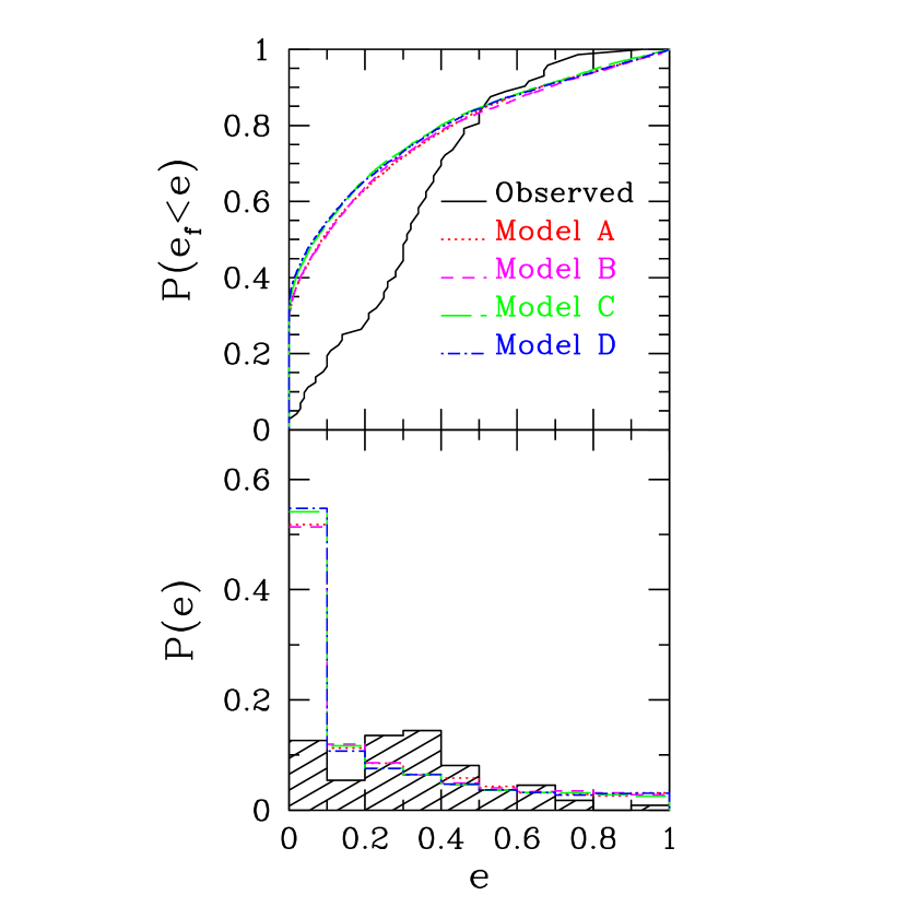
Figure 3: Final cumulative eccentricity distribution (top) and normalized probability distribution histogram (bottom), for four models assuming different fractions of brown dwarf and stellar companions. The frequency of brown dwarfs increases from 5% in model A to 30% in model D. All the brown dwarfs are assumed to reside within $100-2000\,$AU from the primary. The Kozai mechanism produces a much larger population of nearly circular orbits ($e_{1}<0.1$) than in the observed sample. Also evident in the histogram is a slight excess of highly eccentric orbits ($e>0.7$) and deficit of intermediate values ($e=0.3-0.5$) created by our models. Larger fractions of brown dwarf companions account for a higher chance of failure of the Kozai oscillation, resulting in more planets remaining on circular orbits.

The first four models have initial parameter distributions that (i) are compatible with our current knowledge of stellar and substellar binary companions, and (ii) can produce the closest result to the observed eccentricity distribution of extrasolar planets. The results are shown in Figure 3. Each of the four different models represents 5000 sample systems with a different assumed ratio of brown dwarf companions to FGK dwarf companions. Although the differences between these models are rather small, the results show that a higher fraction of brown dwarf companions leads to more planets with low eccentricities, as expected. All the models produce a large excess of planets with eccentricity less than 0.1, more than 50% of the total planets, compared to only 15% in the observed sample (excluding multiple-planet systems).

Table 3 shows statistics for our models compared to the observed sample. Clearly the median eccentricity of the models significantly differs from that of the observed planets. According to the observational estimate by Gizis et al. (2001), the brown dwarf frequency among companions of FGK dwarfs can vary from approximately 5% to 30%. Even with the smallest fraction of brown dwarf companions in the sample, the Kozai mechanism still fails to produce more than 50% of planets with final eccentricities higher than 0.1. For the population of systems with $e_{1}>0.6$, the models show much better agreement with observations than in the lower eccentricity regime, although there is a slight excess of highly eccentric orbits created by the Kozai mechanism. It is also evident in the histogram that our models have a deficit in the population of intermediate eccentricities ($e_{1}=0.2-0.6$), compared to the observed sample. This can be attributed to the fact that during the Kozai oscillation, the eccentricity of the planet spends more time at very high and very low eccentricities than at intermediate values.

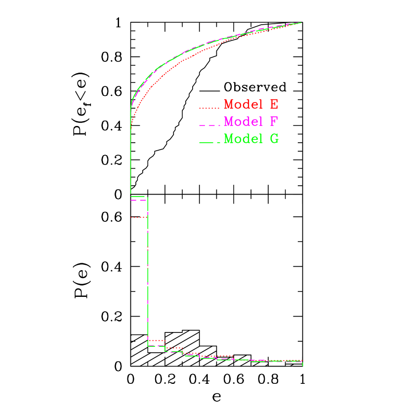
Figure 4: Comparison of models with different semimajor axis distributions. In models E, F and G, the semimajor axes of the companions are distributed uniformly in $\log{a_{2}}$, up to 2000, 6000, and $10,000\,$AU, respectively. As a binary companion is more distant from the primary, the Kozai period increases and the eccentricity oscillation is more likely to be suppressed. A companion at a distance farther than about $6000\,$AU from the primary is rarely effective in perturbing the planet’s orbit into an eccentricity oscillation. Note that in model G, only about $35\%$ of the planets have final eccentricities higher than 0.1.

The effect of different distributions of $a_{2}$ is shown in Figure 4. The models have different upper limits for $a_{2}$; 2000, 6000, and $10000\,$AU in models E, F, and G, respectively. Recall that, since the Kozai period (eq. [2]) is sensitive to $a_{2}$, the choice of distribution of $a_{2}$ can significantly affect the distribution of final eccentricities. Binary systems with separations as large as $\sim 10000\,$AU have been observed, but the frequency of such wide binaries is very poorly constrained. Note that model G shows over 50% more planets with nearly circular orbits. In this model, binary companions are largely populated beyond the effective range of the Kozai mechanism, and more than 25% of the planets fail to complete one eccentricity oscillation cycle during the lifetime of the system.

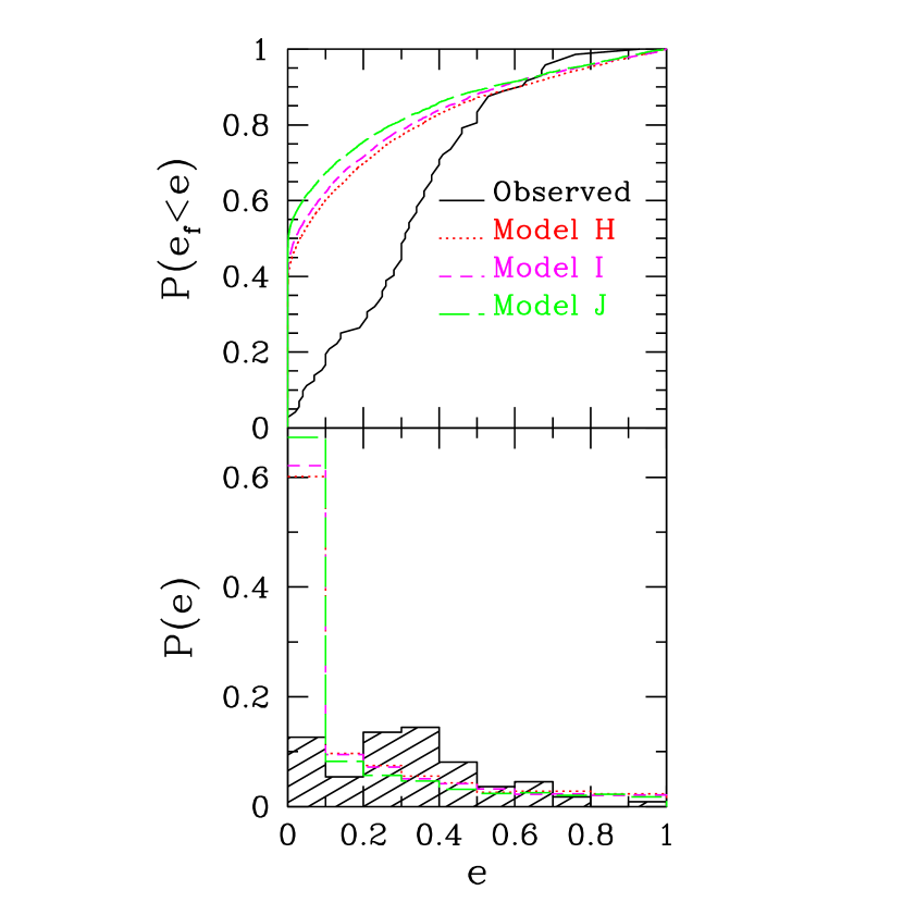
Figure 5: Comparison of different sizes of brown dwarf deserts. Here, 30% of companions are brown dwarfs and the rest are stellar companions. In model H, I and J, brown dwarf companions exist only beyond 10, 100, and $1000\,$AU from the primary, respectively. Currently, very few brown dwarf companions have been observed within $100-1000\,$AU from solar-type stars. A brown dwarf companion in general needs to be within $\sim 1000\,$AU of the primary star to perturb the planet’s orbit significantly within the lifetime of the system. Model J, in which brown dwarf companions are all located farther than $1000\,$AU away from the primary, has nearly 50% of the planets remaining in nearly circular orbits.

Figure 5 presents models with varying brown dwarf deserts. Each model contains no brown dwarf companions within a distance of 10, 100, or $1000\,$AU from the primary. As mentioned in §2.1, observationally, the brown dwarf desert is likely to extend to $100-1000\,$AU. Note that the discrepancy in the population of near-circular orbits becomes smaller when there are more brown dwarfs at closer separations. Recall that the Kozai oscillation caused by a brown dwarf companion has a period typically 10-100 times longer than that caused by a main-sequence star companion. A brown dwarf companion at a distance of $1000\,$AU has about the same effect on a planet as does a solar-like companion at $2000-4000\,$AU. Thus, if we continue to discover close brown dwarf companions (e.g., Endl et al. (2004)), this could be responsible for 5%-10% more planets being perturbed to $e>0.1$.

A major discrepancy between most of the simulated and observed eccentricity distributions occurs in the low-eccentricity regime ($e<0.1$). This discrepancy mainly arises from a large population of binary companions with initial orbital inclinations less than the critical value, resulting in no secular perturbation. Note that the observed fraction of planets with nearly circular orbits is 23% (or only 15% if we exclude multiple-planet systems). In our models, the isotropic distribution of $i_{0}$ implies that there are also about 23% of the systems with $i_{0}<39.23^{\circ}$. However, a much higher fraction of model systems fail to reach high eccentricities since, even with $i_{0}>40^{\circ}$, Kozai perturbations are not always significant. Hence, the Kozai mechanism fails to explain this small population of observed near-circular orbits unless there is some unknown correlation between the orbital planes of the planets and the distant companions that results in an anisotropic distribution of $i_{0}$, with high relative inclinations preferred.

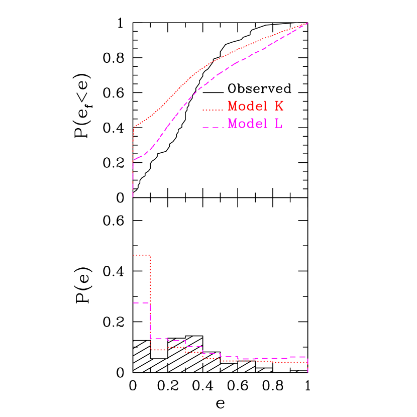
Figure 6: Biased distributions of initial inclination angles and initial eccentricities of the companions. For both simulations, inclination angles are initially distributed uniformly in $\cos{i_{0}}$ between $50^{\circ}$ and $80^{\circ}$. Companions are all brown dwarfs in model K, and 5% brown dwarfs and 95% FGK dwarfs in model L. For both models, all the companions have high initial orbital eccentricities ($e_{2}>0.75$) so as to decrease the eccentricity oscillation period. Model L shows the smallest deviation from the observed sample in the low and intermediate-eccentricity regions, but the agreement is rather poor for $e>0.6$.

In models K and L we have adopted artificially biased distributions of $i_{0}$ and $e_{2}$ to achieve the best possible agreement with the observations. In these models, all the systems initially have uniform $\cos{i_{0}}$ distribution, but all are concentrated in the range $50^{\circ}-80^{\circ}$. The initial eccentricities of the companions are from a thermal distribution but only above 0.75, so as to decrease the average Kozai period. In model K, all the binary companions are brown dwarfs, and in model L, 5% are brown dwarfs and 95% are FGK dwarfs. The result is shown in Figure 6. Model L produced the smallest fraction planets with $e_{1}<0.1$ among all our models. This model also has the smallest deviation from observations in the intermediate-eccentricity regime. Nevertheless, this biased model still created an overabundance of nearly circular orbits compared to the observations, by about $7\%$. Although all the systems in the model undergo eccentricity oscillations and about 95% have Kozai periods short compared to the age of the system, in 14% of the systems oscillations are suppressed by GR precession. Also, as noted in columns (10) and (11), labeled “unlucky” in Table 2, 11% of the planets have successfully undergone eccentricity oscillations, yet would, just by chance, be observed when their orbits are nearly circular. With these two factors combined, an excess of simulated systems with eccentricities $<0.1$ still cannot be avoided. Also note (in the histogram) that, while producing better agreement with the observed sample in the low-eccentricity regime, model L has created the largest excess observed in the high-eccentricity regime ($e>0.6$). These extreme models are clearly artificial, and our aim here is merely to quantify how large a bias would be needed to match the observations “at any cost.”

4 Summary and Discussion

For each of our simulated samples, we have run a Kolmogorov-Smirnov test, which provides the probability that a model is derived from the same underlying population as the observed sample. Not surprisingly, none of our models have produced a significance level higher than 1%, the highest being 0.03% for model L. However, it is interesting to examine more closely the source of the discrepancy in the low-eccentricity ($e<0.1$) and high-eccentricity ($e>0.6$) regimes.

In most of our simulations, the Kozai mechanism tends to overproduce planets with very low orbital eccentricities. The lowest quartile of final eccentricities in any of the models is much less than 0.1, whereas in the observed sample this is 0.14. There are several reasons for this overabundance of low eccentricities in our model systems. First, since we do not have any observational constraints on relative inclination angles, we have assumed an isotropic distribution of $i_{0}$. This implies that $23\%$ of the systems have $i_{0}<i_{\rm crit}$, resulting in no Kozai oscillation. However, in the total observed sample, planets with $e_{1}<0.1$ are only 23% of the total (or 15% if we exclude multi-planet systems and hot Jupiters with $a_{1}<0.1\,$AU). Systems with sufficient initial relative inclination angles still need to overcome other hurdles to achieve highly eccentric orbits. If many of the binary companions are substellar or in very wide orbits, Kozai periods become so long that the eccentricity oscillation are either suppressed by GR precession, or not completed within the age of the system (or both). This can result in an additional 15%-40% of planets remaining in nearly circular orbits. Even when the orbits of the planets do undergo eccentricity oscillations, about 8-14% just happen to be observed at low eccentricities. Thus, our results suggest that the observed sample has a remarkably small population of planets in nearly circular orbits, and other dynamical processes must clearly be invoked to perturb their orbits. Among the most likely mechanisms is planet–planet scattering in multi-planet systems, which can easily perturb eccentricities to modest values in the intermediate range $\sim 0.2-0.6$ (Rasio & Ford, 1996; Weidenschilling & Marzari, 1996; Marzari & Weidenschilling, 2002). Clear evidence that planet–planet scattering must have occurred in the $\upsilon$ Andromedae system has been presented by Ford, Lystad, & Rasio (2005). Even in most of the systems in which only one giant planet has been detected so far, the second planet could have been ejected as a result of the scattering, or it could have been retained in a much wider, eccentric orbit, making it hard to detect by Doppler spectroscopy.

In the high-eccentricity region, where $e_{1}\gtrsim 0.6$, our models show much better agreement with the observed distribution. The Kozai mechanism predicts a small excess of systems at the highest eccentricities ($e>0.8$), although it should be noted that the observed eccentricity distribution in this range is not yet well constrained. It is evident that the observed planets are rather abundant in intermediate values of eccentricity. Nearly half the extrasolar planets are observed with eccentricities between 0.15 and 0.40. The Kozai mechanism tends to populate somewhat higher eccentricities, since during the eccentricity oscillation planets spend more time around $e_{1,\rm max}$ than at intermediate values. However, this slight excess of highly eccentric orbits could easily be eliminated by invoking various circularization processes. For example, some residual gas may be present in the system, leading to circularization by gas drag (Adams & Laughlin, 2003), or planets perturbed to highly eccentric orbits could be induced to collide with other planets farther in, thereby also reducing their final eccentricities.

Our two models with inclination angle distributions biased toward higher values (models K and L) come a bit closer to reproducing the observed eccentricity distribution, as expected. In model L we have managed to shift the simulated cumulative distribution closer to the observations in the low-eccentricity regime, but at the cost of an even larger discrepancy at high eccentricities. Clearly, even by stretching our assumptions, it is not possible to explain the observed eccentricity distribution of extrasolar planets solely by invoking the presence of binary companions, even if these companions are largely undetected or unconstrained by observations. However, our models suggest that Kozai-type perturbations could play an important role in shaping the eccentricity distribution of extrasolar planets, especially at the high end. In addition, they predict what the eccentricity distribution for planets observed around stars in wide binary systems should be. The frequency of planets in binary systems is still very uncertain, but new distant companions to stars with known planetary systems are being discovered all the time, and searches for planets in binary stars are ongoing (Mugrauer et al., 2004; mug04b; egg04).

Figure 1: Constraints in the orbital parameter space imposed for the Kozai mechanism to be effective. Solid lines represent the limits above which the Kozai oscillation is too slow, so the planet does not have enough time to complete one eccentricity oscillation cycle within the lifetime of the triple system. Similarly, above the dashed lines, the relativistic precession period is shorter than the Kozai period, and the Kozai oscillation is suppressed. The constraints become tighter as the binary companion mass decreases. Shorter orbital periods for the planet also tighten the constraints.

Figure 2: Eccentricity oscillation of a planet caused by a distant brown dwarf companion ($M=0.08M_{\odot}$, solid line) and by a main-sequence dwarf companion ($M=0.9M_{\odot}$, dotted line). For both cases, the mass of the planet host star $m_{0}=1M_{\odot}$, the planet mass $m_{1}=1M_{\rm J}$, the planet semimajor axis $a_{1}=2.5\,$AU, the semimajor axis of the companion $a_{2}=750\,$AU, the initial eccentricity of the companion $e_{2}=0.8$, and the initial relative inclination $i_{0}=75^{\circ}$. Note that $e_{1,\rm max}$ remains nearly constant, as it is dependent only on $i_{0}$. The smaller mass of a brown dwarf companion results in a much longer oscillation period $P_{\rm KOZ}$.

Table 1: Model Parameters

Model	$a_{2,\rm FGK}$	$a_{2,\rm BD}$	$e_{2}$	$i_{0}$	BDs
A	using $P_{2}$, $<2000\,$AU	$100-2000\,$AU	$10^{-5}$ - 0.99	isotropic	250(5%)
B	using $P_{2}$, $<2000\,$AU	$100-2000\,$AU	$10^{-5}$ - 0.99	isotropic	500(10%)
C	using $P_{2}$, $<2000\,$AU	$100-2000\,$AU	$10^{-5}$ - 0.99	isotropic	1000(20%)
D	using $P_{2}$, $<2000\,$AU	$100-2000\,$AU	$10^{-5}$ - 0.99	isotropic	1500(30%)
E	$10-2000\,$AU	$100-2000\,$AU	$10^{-5}$ - 0.99	isotropic	500(10%)
F	$10-6000\,$AU	$100-6000\,$AU	$10^{-5}$ - 0.99	isotropic	500(10%)
G	$10-10000\,$AU	$100-10000\,$AU	$10^{-5}$ - 0.99	isotropic	500(10%)
H	using $P_{2}$, $10-4000\,$AU	$100-4000\,$AU	$10^{-5}$ - 0.99	isotropic	1500(30%)
I	using $P_{2}$, $100-4000\,$AU	$100-4000\,$AU	$10^{-5}$ - 0.99	isotropic	1500(30%)
J	using $P_{2}$, $1000-4000\,$AU	$100-4000\,$AU	$10^{-5}$ - 0.99	isotropic	1500(30%)
K	—	$10-2000\,$AU	0.75 - 0.99	$50^{\circ}-80^{\circ}$	5000(100%)
L	—	$10-2000\,$AU	0.75 - 0.99	$50^{\circ}-80^{\circ}$	250(5%)

Table 2: Systems with low eccentricities

Model	$e_{1}<0.1$	$i_{0}<i_{\rm KOZ}$	$P_{\rm KOZ}>age$	$P_{\rm KOZ}<P_{\rm GR}$	unlucky
obs	11/72 (15.3%)	—	—	—	—
A	2590 (51.8%)	1115 (22.3%)	316 (6.32%)	701 (14.0%)	708 (14.1%)
B	2569 (51.3%)	1109 (22.2%)	365 (7.30%)	761 (15.2%)	615 (12.3%)
C	2692 (53.8%)	1180 (23.6%)	410 (8.20%)	775 (15.5%)	612 (12.2%)
D	2751 (55.0%)	1109 (22.2%)	450 (9.00%)	858 (17.2%)	606 (12.1%)
E	2992 (59.8%)	1188 (23.8%)	519 (10.4%)	913 (18.3%)	639 (12.8%)
F	3329 (66.6%)	1146 (22.9%)	1099 (22.0%)	1320 (26.4%)	531 (10.6%)
G	3406 (68.1%)	1107 (22.1%)	1295 (25.9%)	1490 (29.8%)	490 (9.80%)
H	3005 (60.1%)	1162 (23.2%)	777 (15.5%)	1061 (21.2%)	554 (11.1%)
I	3104 (62.1%)	1126 (22.5%)	901 (18.0%)	1166 (23.3%)	578 (11.6%)
J	3363 (67.3%)	1120 (22.4%)	1381 (27.6%)	1511 (30.2%)	465 (9.30%)
K	2131 (42.6%)	0 (0%)	960 (19.2%)	1494 (29.9%)	398 (7.96%)
L	1372 (27.4%)	0 (0%)	260 (5.20%)	704 (14.1%)	591 (11.8%)

Note. — Analysis of the model population of planets with final eccentricities $e_{\rm f}<0.1$. Percentages represent the ratio of planets with $e_{\rm f}<0.1$ to the total number of sample systems. The first row is for the observed sample from the California & Carnegie Planet Search Catalogue, excluding the tight-orbit planets ($a_{1}<0.1\,$AU) and multi-planet systems. The second column gives the number of planets with $e_{\rm f}<0.1$. The third column gives the number of planets with initial inclination angles below the critical value ($i_{0}<i_{\rm KOZ}$). The fourth column gives the number of systems that could not reach the first maximum of the eccentricity oscillation within the lifetime of the system. The fifth column gives the number of systems whose Kozai oscillation is suppressed by GR precession. The last column gives the number of planets that have undergone Kozai oscillations, but for which the final eccentricity still happens to be low, with $e_{\rm f}<0.1$.

Table 3: Statistics of eccentricity distributions

Model	Mean	First quartile	median	Third quartile
observed	0.323	0.140	0.310	0.440
A	0.213	0.000	0.087	0.348
B	0.215	0.000	0.091	0.341
D	0.203	0.000	0.066	0.327
E	0.175	0.000	0.040	0.266
F	0.140	0.000	0.004	0.186
G	0.141	0.000	0.001	0.184
H	0.175	0.000	0.033	0.265
I	0.163	0.000	0.020	0.241
J	0.144	0.000	0.002	0.192
K	0.245	0.000	0.141	0.416
L	0.341	0.071	0.270	0.559

References

- Adams & Laughlin (2003) Adams, F.C., & Laughlin, G. 2003, Icarus, 163, 290
- Belczynski et al. (2002) Belczyinski, K., Kalogera, V., & Bulik, T. 2002, ApJ, 572, 407
- Chiang & Murray (2002) Chiang, E.I., & Murray, N. 2002, ApJ, 576, 473
- Delgado-Donate (2004) Delgado-Donate, E.J., Clarke, C.J., Bate, M.R., & Hodgkin, S.T. 2004, MNRAS, 351, 617
- Donahue (1998) Donahue, R.A. 1998, APS Conference Series, 154, 1235
- Duquennoy & Mayor (1991) Duquennoy, A., & Mayor, M. 1991, A&A, 248, 485
- Endl et al. (2004) Endl, M, Hatzes, A.P., Cochran, W.D., McArthur, B., Prieto, C.A., Paulson, D.B., Guenther, E., & Bedalov, A. 2004, ApJ, 611, 1121
- Fischer & Marcy (1992) Fischer, D.A., & Marcy, G.W. 1992 ApJ, 396, 178
- Ford et al. (2000) Ford, E.B., Kozinsky, B., & Rasio, F.A. 2000, ApJ, 535, 385; erratum 2004, ApJ, 605, 966 303
- Ford et al. (2005) Ford, E.B., Lystad, V., & Rasio, F.A. 2005, Nature, in press
- Gizis et al. (2001) Gizis, J.E., Kirkpatrick, J.D., Burgasser, A., Reid, I.N., Monet, D.G., Liebert, J., & Wilson, J.C. 2001, ApJ, 551, 163
- Halbwachs et al. (2000) Halbwachs, J.L., Arenou, F., Mayor, M., Udry, S., & Queloz, D. 2000, A&A, 355, 581
- Heggie (1975) Heggie, D.C. 1975, MNRAS, 173, 729
- Holman et al. (1997) Holman, M.J., Touma J., & Tremaine, S. 1997, Nature, 386, 254
- Holman & Wiegert (1999) Holman, M.J., & Wiegert, P.A. 1999, AJ, 117, 621
- Ida & Lin (2003) Ida, S., & Lin, D.N.C. 2004, ApJ, 604, 388
- Innanen et al. (1997) Innanen, K.A., Zheng, J.Q., Mikkola, S., & Valtonen, M.J. 1997, AJ, 113, 1915
- Jorissen, Mayor & Udry (2001) Jorissen, A., Mayor, M., & Udry, S. 2001, A&A, 379, 992
- Kozai (1962) Kozai, Y. 1962, AJ, 67, 591
- Lowrance et al. (2002) Lowrance, P.J., Kirkpatrick, J.D., & Beichman, C.A. 2002, ApJ, 572, 79
- Marzari & Weidenschilling (2002) Marzari, F., & Weidenschilling, S.J. 2002, Icarus, 156, 570
- Mugrauer et al. (2004) Mugrauer, M., Neuhäuser, R., Mazeh, Fernández, M.T., & Guenther, E. 2004, in AIP Conf.Proc. 713, The Search for Other Worlds: 14th Astrophysics Conference, ed. S.S.Holt & D.Deming (New York: AIP), 31
- Portegies Zwart & Yungelson (1998) Portegies Zwart, S.F., & Yungelson, L.R. 1998, A&A, 332, 173
- Rasio & Ford (1996) Rasio, F.A., & Ford, E.B. 1996, Science, 274, 954
- Reid et al. (1999) Reid, I.N., et al. 1999, ApJ, 151, 393
- Tabachnik & Tremaine (2002) Tabachnik, S., & Tremaine, S. 2002, MNRAS, 335, 151
- Tremaine & Zakamska (2004) Tremaine, S., & Zakamska, N.L. 2004, The Search for Other Worlds, AIP Conference Proceedings, Vol. 713, 243
- Verbunt & Phinney (1995) Verbunt, F., & Phinney, E.S. 1995, A&A, 296, 709
- Weidenschilling & Marzari (1996) Weidenschilling, S.J., & Marzari, F. 1996, Nature, 384, 619
- Wu & Murray (2003) Wu, Y., & Murray, N. 2003, ApJ, 589, 605
- Zucker & Mazeh (2002) Zucker, S., & Mazeh, T. 2002, ApJ, 568, 113