Possible Explanation to Low CMB Quadrupole

Abstract

The universe might experience many cycles with different vacua. The slow-roll inflation may be preceded by kinetic-dominated contraction occurring in “adjacent” vacua during some cycles. In this report we briefly show this phenomenon may lead to a cutoff of primordial power spectrum, which is mildly preferred by WMAP data. Thus in some sense the CMB at large angular scale might encode the information of other vacua.

The interesting result of recent WMAP data, which confirms earlier COBE observations [1, 2], is a lower amount of power on the largest scales when compared to that predicted by the standard $\Lambda$CDM models [3, 4]. This may be contributed to cosmic variance with bad luck, where we might simply live in a region of universe with the CMB quadrupole happening to be small. However this lower power might also imply a cutoff of primordial power spectrum on the largest scale [5], which is related to the physics before the onset of inflation [6]. There are also many other attempts [7, 8, 9] to explain WMAP data.

Recently, a large number of vacuum states in string theory has received many attentions [10, 11], see also Ref. [12, 13]. The space of all such vacua has been dubbed landscape [14]. In some sense, the low energy properties of string theory can be approximated by field theory. Thus the landscape can also be described as the space of a set of fields with a complicated and rugged potential, where the local minima of potential are called the vacua. When this local minimum is an absolute minimum, the vacuum is stable, and otherwise it is metastable. In string landscape with exponentially large number of vacua we can only live in one vacuum compatible to us, which might make us able to anthropically solve the problem of cosmological constant that has been troubling us for a long time [15, 16]. Further it has been shown in Ref. [17] that for a landscape with a large number of AdS minima the universe may experience many cycles [18] with different minima, when the number of cycles is large or approaches infinity, whichever minimum initially the universe is in, it can run over almost all vacua of the landscape. Thus in some sense the physics of adjacent vacua settles the initial conditions and affects the evolution of universe with the vacua observed. Further this might leave an observable imprint in CMB under certain conditions. We will briefly illustrate this possibility in this report.

For a simplified example given in terms of an order parameter $\varphi$, the effective description of a landscape with many AdS minima can be taken as follows

$${\cal V}(\varphi)=\Lambda_{*}\left(1-\cos({m\over\sqrt{\Lambda_{*}}}\varphi)\right)-\Lambda,$$ (1)

where $\Lambda$ is a small positive constant which makes the minima of periodic potential negative, and $m$ is the mass around the minima of potential. The universe with negative potential will eventually collapse [19]. But Big Crunch singularity might be not a possible feature of quantum gravity. There should be some mechanisms from high energy/dimension theories responsible for a nonsingular bounce. We suppose, following this line, that in high energy regime the Friedmann equation can be modified as $3h^{2}\simeq\rho_{\varphi}-\rho_{\varphi}^{2}/\sigma$ [20], where $8\pi/m_{p}^{2}=1$ has been set, and $\sigma$ is the bounce scale.

Following Ref.[17], the universe, controlled by a rugged potential with many AdS minima and a bounce mechanism in high energy regime, will show itself many contraction/expansion cycles. The functions of the field and scale factor with respect to time are plotted in Fig. 1. When the bounce scale $\sigma$ is larger than the height of potential hill, the field will be driven from a minimum to another, and during each cycle of oscillating universe the field will generally lie in different minima. The kinetic energy of the field during contraction will rise rapidly and be much larger than its potential energy, which makes the field able to get over the potential barrier easily and quickly. The maximum value to which the field is driven during each contraction/expansion cycle can be simply estimated as [17, 21]

$$\varphi_{m}\simeq 1+\sqrt{2\over 3}\ln{({\sigma\over m^{2}})},$$ (2)

which is only relevant with the mass $m$ around its minima and the bounce scale $\sigma$. For the potential of (1), in the apex of hill, $\varphi_{a}={\pi\sqrt{\Lambda_{*}}\over m}$. Thus to make the field $\varphi$ can stride over a potential hill during a cycle, $\varphi_{m}\gtrsim{\pi\sqrt{\Lambda_{*}}\over m}$ has to be satisfied.

Figure 1: The upper left panel is the figure of potential (1) for illustration. The upper right panel is the figure of $\ln{a}$ with respect to time, where $\Lambda_{*}=0.07$, ${m\over\sqrt{\Lambda_{*}}}=1$ and $\Lambda=0.0005$ are taken. The lower left panel is the figure of the value of field with respect to time, while lower right panel is the figure of its potential energy (solid line) and kinetic energy (dashing line) in time interval (25, 40). The field generally oscillates in different minima during different cycles of universe.

We assume that after getting across the potential barrier and before rolling down to its new minimum, the field can enter into a phase dominated by a flat part of potential, which drives a period inflation of universe, see Fig. 2 for an illustration, where $m_{1}$ and $m_{2}$ are the mass scale of two adjacent minima respectively. The potential at the right side of the apex $\varphi_{a}$ of potential hill can be written as $2(\Lambda_{*}-{1\over 2}m^{2}_{2}\varphi^{2})$, which may be regarded as an expansion of Eq. (1)-like potential around $\varphi_{a}$. The e-folds number during the inflation for above potential is

$${\cal N}=\int hdt\simeq{\Lambda_{*}\over m_{2}^{2}}\ln({\varphi_{e}\over\varphi_{i}}),$$ (3)

where $\varphi_{e}$ is the value of field in which the inflation ends, which can be approximately given by the slow-roll parameter $\epsilon\simeq{m_{2}^{4}\varphi^{2}_{e}\over\Lambda_{*}^{2}}\simeq 1$, thus $\varphi_{e}\simeq{\Lambda_{*}\over m_{2}^{2}}$, and $\varphi_{i}$ is the value of field in which the inflation begins, which is determined by the physical parameters of last minimum,

$$\varphi_{i}=\triangle\varphi\simeq\varphi_{m}-{\pi\sqrt{\Lambda_{*}}\over m_{1}}.$$ (4)

From Eq. (4), we can see that in principle the physics of adjacent minima can determine the possibility and e-folds number of inflation in succedent minimum. For $\varphi_{i}=\triangle\varphi<\varphi_{e}$, the inflation will occur, and after the end of inflation, the parameteric resonance [22] of inflaton will lead to the production of a large number of particles. The decay of these particles will reheat the universe to required temperature, and then the standard cosmological evolution begins. The universe will recollapse and enter into next cycle until the energy density of matter is equal to that of AdS minimum.

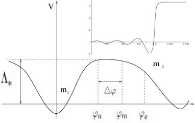
Figure 2: The illustration of model, where $m_{1}$ and $m_{2}$ are the mass scale of two adjacent vacua respectively, and $\varphi_{i}$ is the value of field at the onset of inflation and $\varphi_{e}$ is the value of field in which the inflation ends. The inset is the figure of the value of field with respect to time during a contraction/expansion cycle, where the effective potential is taken as a combination of potential of (1) and a flat potential, which are matched at $\varphi_{a}={\pi\sqrt{\Lambda_{*}}\over m}$, and $\Lambda_{*}=0.07$, ${m\over\sqrt{\Lambda_{*}}}=1$ and $\Lambda=0.001$. Initially the field oscillates in its minima with mass scale $m_{1}$, then roll up along its potential, and after the bounce of universe, the field enters into the slow-roll regime rapidly, in which the mass scale is $m_{2}$.

We then calculate the primordial spectrum of the above model discussed. There are generally two regimes for the generation of primordial spectrum in this model, namely kinetic-dominated phase and succedent inflationary phase. For simplify, we neglect the details of the bounce and pay much attention to an instantaneous transition between both phases. Following [8], the scale factors of two different phases can be given by

$$a\simeq\sqrt{1-2{\cal H}_{0}\eta}~{},~{}~{}~{}~{}~{}\eta\leq 0$$ (5)

$$a\simeq{1\over 1-{\cal H}_{0}\eta}~{},~{}~{}~{}~{}~{}\eta\geq 0$$ (6)

respectively, where $\eta$ is the conformal time, $\eta=0$ and $a=1$ have been set for the matching at the moment of transition, and ${\cal H}_{0}$ is the value of ${\cal H}={a^{\prime}\over a}$ at $\varphi=\varphi_{i}$, in which the universe just enters into inflationary phase.

The variable [23]

$$v\equiv a\left(\delta\varphi+{\varphi^{\prime}\over{\cal H}}\Phi\right)\equiv z\zeta,$$ (7)

is defined for the calculations of perturbation spectrum, where $\Phi$ is the Bardeen potential [26] and $\zeta$ is the curvature perturbation on uniform comoving hypersurface, and $\delta\varphi$ is the perturbations of the scalar field during both phases, and $z\equiv{a\varphi^{\prime}\over{\cal H}}$, see [24, 25] for a thorough introduction to gauge invariant perturbations. In the momentum space, the equation of motion of $v_{k}$ is

$$v_{k}^{\prime\prime}+\left(k^{2}-{z^{\prime\prime}\over z}\right)v_{k}=0.$$ (8)

For the kinetic-dominated contracting phase,

$${z^{\prime\prime}\over z}\simeq{a^{\prime\prime}\over a}\simeq{-{\cal H}_{0}^{2}\over(1-2{\cal H}_{0}\eta)^{2}}.$$ (9)

When $k^{2}\gg{z^{\prime\prime}\over z}$, the fluctuations are deep in the contracting phase and can be taken as an adiabatic vacuum, which corresponds to

$$v_{k}\sim{1\over\sqrt{2k}}e^{-ik\eta},$$ (10)

thus

$$v_{k}(\eta)=\sqrt{\pi(1-2{\cal H}_{0}\eta)\over 8{\cal H}_{0}}{\cal H}_{0}^{(2)}\left(-k\eta+{k\over 2{\cal H}_{0}}\right),$$ (11)

where ${\cal H}_{0}^{(2)}$ is the second kind of Hankel function with $0$ order. For the nearly de Sitter phase,

$${z^{\prime\prime}\over z}\simeq{a^{\prime\prime}\over a}\simeq{2{\cal H}_{0}^{2}\over(1-{\cal H}_{0}\eta)^{2}},$$ (12)

thus

$$v_{k}(\eta)=\sqrt{-k\eta+{k\over{\cal H}_{0}}}$$

$$\left(C_{1}{\cal H}_{3\over 2}^{(1)}(-k\eta+{k\over{\cal H}_{0}})+C_{2}{\cal H}_{3\over 2}^{(2)}(-k\eta+{k\over{\cal H}_{0}})\right),$$ (13)

where ${\cal H}_{3\over 2}^{(1)}$ and ${\cal H}_{3\over 2}^{(2)}$ are the first and second kind of Hankel function with ${3\over 2}$ order respectively, $C_{1}$ and $C_{2}$ are the functions dependent of $k$, and are determined by the matching conditions between both phases, which are related to the physics around the bounce and specifically depend on which of $\zeta$ and $\Phi$ passes regularly through the bounce [27]. The continuities of $v$ and $v^{\prime}$ [28] at the transition give

$$C_{1}= \sqrt{\pi\over 32{\cal H}_{0}}e^{-ik\over{\cal H}_{0}}((1-{2{\cal H}_{0}^{2}\over k^{2}}-{2{\cal H}_{0}\over k}i){\cal H}_{0}^{(2)}\left({k\over 2{\cal H}_{0}}\right)$$ (14)

$$+({{\cal H}_{0}\over k}+i){\cal H}_{1}^{(2)}\left({k\over 2{\cal H}_{0}}\right)),$$

$$C_{2} = \sqrt{\pi\over 32{\cal H}_{0}}e^{ik\over{\cal H}_{0}}((1-{2{\cal H}_{0}^{2}\over k^{2}}+{2{\cal H}_{0}\over k}i){\cal H}_{0}^{(2)}\left({k\over 2{\cal H}_{0}}\right)$$ (15)

$$+({{\cal H}_{0}\over k}-i){\cal H}_{1}^{(2)}\left({k\over 2{\cal H}_{0}}\right)),$$

where ${\cal H}_{0}^{(2)}$ and ${\cal H}_{1}^{(2)}$ are the second kind of Hankel function with $0$ and $1$ order respectively.

The perturbation spectrum is

$${\cal P}_{s}={k^{3}\over 2\pi^{2}}|{v\over a}|^{2}$$ (16)

for $\eta\rightarrow 1/{\cal H}_{0}$. Substituting (13), (14) and (15) into (16), we obtain

$${\cal P}_{s}={{\cal H}_{0}^{2}\over 2\pi^{2}}k|C_{1}-C_{2}|^{2}.$$ (17)

For $k\ll{\cal H}_{0}$, the Hankel function can be expanded in term of large variable, thus we obtain approximately $P_{s}\sim k^{3}$ on large scale, which is the usual result of PBB scenario [29]. For $k\gg{\cal H}_{0}$, the expansion of small variable of the Hankel function gives $P_{s}\sim k^{0}$ i.e. nearly scale-invariant spectrum on small scale. The result of numerical calculation is plotted in inset of Fig. 3, where the cutoff of spectrum can be seen clearly, which is consistent with above semianalytical ones. The large $k$ modes are generally inside the horizon during the kinetic-dominated phase and are not quite sensitive to the background at this stage. Thus when they cross the horizon during inflation after the transition, the nearly scale-invariant spectrum can be generated by the evolution of the background during inflationary phase.

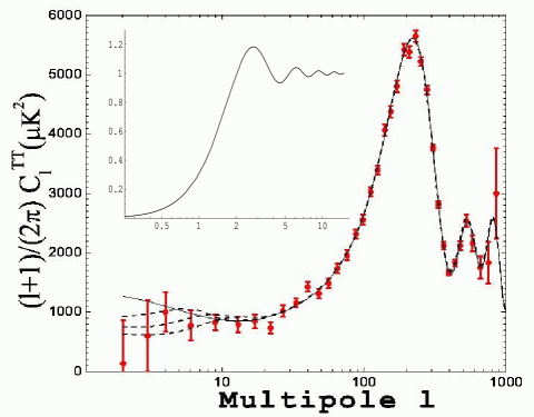
Figure 3: The CMB anisotropy for the scale-invariant spectrum and the spectrum with a cutoff. From left top to bottom, the lines stand for scale-invariant spectrum, spectrum with a cutoff with ${\cal H}_{0}=2.1,3.1$ and $4.1\times 10^{-4}$ Mpc^-1. The other parameters are fixed at $h=0.73$, $\Omega_{b}h^{2}=0.023$, $\Omega_{cdm}h^{2}=0.117$ and $\tau=0.2$. The inset is the power spectrum ${\cal P}_{s}$as a function of ${k\over{\cal H}_{0}}$. The x-axe is ${k\over{\cal H}_{0}}$, and the y-axe is ${\cal P}_{s}/\left({{\cal H}_{0}\over 2\pi}\right)^{2}$.

We fit the resulting primordial spectrum to the current WMAP data. In Fig. 3, we show the CMB TT multipoles for the scale-invariant spectrum and the cutoff spectrum with various ${\cal H}_{0}$. Regarded as a cutoff scale in the spectrum, ${\cal H}_{0}$ can be chosen as ${\cal H}_{0}\lesssim 5.0\times 10^{-4}$ Mpc^-1 in our fit. From Fig. 3, we see that the lower CMB TT quadrupole is related to the value of ${\cal H}_{0}$, which can be determined by Eq. (4). Thus in some sense lower CMB quadrupole encodes the information of adjacent vacua. In addition we get a minimum $\chi^{2}=1428.2$ at $h=0.73$, $\Omega_{b}h^{2}=0.024$, $\Omega_{cdm}h^{2}=0.116$, $\tau=0.2$ and ${\cal H}_{0}=2.0\times 10^{-4}$ Mpc^-1. We also run a similar code for the scale-invariant spectrum for comparison and get a minimum $\chi^{2}=1429.7$ at $h=0.73$, $\Omega_{b}h^{2}=0.024$, $\Omega_{cdm}h^{2}=0.116$ and $\tau=0.2$. This means the primordial spectrum in our example is favored at $>1.22\sigma$ than the scale-invariant spectrum.

We notice that the errors in power spectrum estimates, especially at low l, are highly non-Gaussian, thus the model depends in a nonlinear way on the parameters, which to some extent makes our simply numerical analysis incorrect. To assign a statistical significance correctly, either Monte Carlo simulations or a full Bayesian analysis is necessary. However, this brief report is not primarily about these statistical issues, thus a Numerical-Recipes-level analysis may be enough.

Though our model does not solve the problem of the low CMB quadrupole completely, it provides a mechanism leading to the cutoff of primordial power spectrum, which in some sense is mildly preferred by WMAP data. The suppression of CMB quadrupole in our model is significantly dependent of parameters of adjacent minima. However, since the number of vacua in the landscape is exponentially large, there may always exist some adjacent vacua with such characters, thus the probability that an observer finds a suppression with intension observed will be not too small, which in some sense relaxes the requirement for fine-tuning.

Facing diverse vacua [14] to which string theory brings us, what people might very long for is “seeing” adjacent or other parts of landscape. Thus trying to read some information of other parts from observations will be an excited thing. Though the example in this brief report may be idealistic and speculative, it might identified some of the basic ingredient of required answer. We leave the realistic implementations [30] and other interesting applications to future works.

Acknowledgments The author thank Bo Feng for helpful discussions and kindly offer of CMB anisotropy figure (Fig.3). This work is supported in part by K.C. Wang Posdoc Foundation, also in part by NNSFC under Grant No: 10405029 , 90403032 and by National Basic Research Program of China under Grant No: 2003CB716300 .

References

- [1] C.L. Bennett et.al., Astrophys. J. 464, L1 (1996).
- [2] Y.P. Jing and L.Z. Fang, Phys. Rev. Lett. 73,1882 (1994);
- [3] C. L. Bennett et al., astro-ph/0302207;
- [4] D. N. Spergel et al., astro-ph/0302209;
- [5] S. L. Bridle, A. M. Lewis, J. Weller, and G. Efstathiou, astro-ph/0302306.
- [6] C. R. Contaldi, M. Peloso, L. Kofman, and A. Linde, astro-ph/0303636; J.M. Cline, P. Crotty and J. Lesgourgues, astro-ph/0304558.
- [7] B. Feng and X. Zhang, Phys.Lett.B 570, 145 (2003); M. Kawasaki and F. Takahashi, hep-ph/0305319; G. Efstathiou, astro-ph/0306431; T. Moroi and T. Takahashi,astro-ph/0308208; A. Oliveira-Costa, M. Tegmark, M. Zaldarriaga and A. Hamilton,astro-ph/0307282; S. Tsujikawa, R. Maartens and R. Brandenberger, astro-ph/0308169; Q. Huang and M. Li, astro-ph/0308458; N. Kogo, M. Matsumiya, M. Sasaki, J. Yokoyama, astro-ph/0309662; Q.G. Huang and M. Li, astro-ph/0311378; A. Shafieloo and T. Souradeep, astro-ph/0312174; C.Y. Chen, B. Feng, X.L. Wang, Z.Y. Yang, astro-ph/0404419; M. Liguori, S. Matarrese, M. Musso, A. Riotto, JCAP 0408, 011 (2004); K. Enqvist, M.S. Sloth, hep-th/0406019; C. Gordon, Wayne Hu, Phys.Rev.D70, 083003 (2004); M. Kawasaki, F. Takahashi, T. Takahashi, astro-ph/0407631; P. Hunt and S. Sarkar, Phys.Rev. D70 (2004) 103518; N. Kogo, M. Sasaki, J. Yokoyama, astro-ph/0409052.
- [8] Y.S. Piao, B. Feng and X. Zhang, Phys. Rev. D69 103520 (2004).
- [9] Y.S. Piao, S. Tsujikawa, X. Zhang, Class.Quant.Grav. 21 (2004) 4455.
- [10] M.R. Douglas, JHEP 0305 046 (2003).
- [11] S. Kachru, R. Kallosh, A. Linde and S.P. Trivedi, Phys. Rev. D68 046005 (2003).
- [12] R. Bousso and J. Polchinski, JHEP 0006, 006 (2000); J.L. Feng, J. March-Russell, S. Sethi and F. Wilczek, Nucl. Phys. B602, 307 (2001).
- [13] A.R. Frey, M. Lippert and B. Williams, Phys. Rev. D68, (2003) 046008.
- [14] L. Susskind, hep-th/0302219; B. Freivogel and L. Susskind, hep-th/0408133.
- [15] S. Weinberg, Phys. Rev. Lett. 59, 2607 (1987); Phys. Rev. D61 103505 (2000).
- [16] H. Martel, P. Shapiro and S. Weinberg, Astrophys. J. 492, 29 (1998).
- [17] Y.S. Piao, Phys. Rev. D70, 101302 (2004).
- [18] Recently, the cyclic model has been proposed as a radical alternative to inflation scenario, see J. Khoury, B.A. Ovrut, P.J. Steinhardt and N. Turok, Phys. Rev. D64 (2001) 123522; P.J. Steinhardt and N. Turok, Science 296, (2002) 1436; Phys. Rev. D65 126003 (2002); see also P.J. Steinhardt and N. Turok, astro-ph/0404480 for a recent review.
- [19] G. Felder, A. Frolov, L. Kofman and A. Linde, Phys. Rev. D66 023507 (2002).
- [20] Y. Shtanov and V. Sahni, Phys. Lett. B557 1 (2003).
- [21] Y.S. Piao and Y.Z. Zhang, gr-qc/0407027.
- [22] L. Kofman, A. Linde and A.A. Starobinsky, Phys.Rev.Lett. 73 (1994) 3195; L. Kofman, A.D. Linde and A.A. Starobinsky, Phys. Rev. D56, 3258 (1997).
- [23] V.F. Mukhanov, JETP lett. 41, 493 (1985); Sov. Phys. JETP 67, 1297 (1988).
- [24] H. Kodama and M. Sasaki, Prog. Theor. Phys. Suppl. 78 1 (1984).
- [25] V.F. Mukhanov, H.A. Feldman and R.H. Brandenberger, Phys. Rept. 215, 203 (1992).
- [26] J.M. Bardeen, Phys. Rev. D 22, 1882 (1980).
- [27] C. Cartier, R. Durrer and E.J. Copeland, Phys. Rev. D 67, 103517 (2003).
- [28] For a bounce scenario like PBB see [29] with higher order correction terms, it has been shown to the first order in on the continuity of the induced metric and the extrinsic curvature crossing the constant energy density matching surface between the contracting and the expanding phase, which means that (thus ) passes regularly through the transition. See C. Cartier, J.C. Hwang and E.J. Copeland, Phys. Rev. D 64, 103504 (2001); S. Tsujikawa, R. Brandenberger and F. Finelli, Phys. Rev. D 66, 083513 (2002).
- [29] M. Gasperini and G. Veneziano, Astropart. Phys. 1 (1993) 317, hep-th/9211021; For a review see G. Veneziano, hep-th/0002094; J.E. Lidsey, D. Wands and E.J. Copeland, Phys. Rept. 337 (2000) 343, hep-th/9909061. M. Gasperini and G. Veneziano, hep-th/0207130.
- [30] Y.S. Piao, gr-qc/0502006.