Magnetospheric Eclipses in the Binary Pulsar J0737$-$3039

Abstract

In the binary radio pulsar system J0737$-$3039, the faster pulsar A is eclipsed once per orbit. A clear modulation of these eclipses at the 2.77 s period of pulsar B has recently been discovered. We construct a simple geometric model which successfully reproduces the eclipse light curves, based on the idea that the radio pulses are attenuated by synchrotron absorption on the closed magnetic field lines of pulsar B. The model explains most of the properties of the eclipse: its asymmetric form, the nearly frequency-independent duration, and the modulation of the brightness of pulsar A at both once and twice the rotation frequency of pulsar B in different parts of the eclipse. This detailed agreement confirms the dipolar structure of the star’s poloidal magnetic field. The inferred parameters are: inclination angle between the line of sight and orbital plane normal $\sim 90.5^{\circ}$; inclination of pulsar B rotation axis to the orbital plane normal $\sim 60^{\circ}$; and angle between the rotation axis and magnetic moment $\sim 75^{\circ}$. The model makes clear predictions for the degree of linear polarization of the transmitted radiation.

The weak frequency dependence of the eclipse duration implies that the absorbing plasma is relativistic, with a density much larger than the corotation charge density. Such hot, dense plasma can be effectively stored in the outer magnetosphere, where cyclotron cooling is slow. The gradual loss of particles inward through the cooling radius is compensated by an upward flux driven by a fluctuating component of the current, and by the pumping of magnetic helicity on the closed field lines. The trapped particles are heated to relativistic energies by the damping of magnetospheric turbulence and, at a slower rate, by the absorption of the radio emission of the companion pulsar. A heating mechanism is outlined which combines electrostatic acceleration along the magnetic field with the emission and absorption of wiggler radiation by charged particle bunches.

1 Introduction

The double pulsar system PSR J0737$-$3039A/B contains a recycled 22.7 ms pulsar (A) in a 2.4 hr orbit around a 2.77 s pulsar (B) (Burgay et al., 2003; Lyne et al., 2004). Pulsar A is eclipsed once per orbit, for a duration of $\sim 30$ s centered around superior conjunction. The width of the eclipse is a weak function of the observing frequency (Kaspi et al., 2004). Recently, the pulsar A radio flux has been found to be modulated by the rotation of pulsar B during the eclipse (McLaughlin et al., 2004). The eclipse is longer when the magnetic axis of pulsar B is approximately aligned with the line of sight (assuming that radio pulses are generated near the magnetic axis of B). In addition, there are narrow, transparent windows in which the flux from pulsar A rises nearly to the unabsorbed level. These spikes in the radio flux are tied to the rotation of pulsar B, and provide key constraints on the geometry of the absorbing plasma.

The physical width of the region which causes this periodic modulation is comparable to, or smaller, than the estimated diameter of the magnetosphere of pulsar B. Combined with the rotational modulation, this provides a strong hint that the absorption is occurring within the magnetosphere of pulsar B, which retains enough plasma to effect an eclipse. An alternative possibility, which we disfavor, is that the eclipse is caused by absorption in the relativistic wind of pulsar A after it is shocked and decelerated by its interaction with the magnetosphere of B (Lyutikov, 2004; Arons et al., 2004).

Distinguishing between these two models is greatly aided by a quantitative model of the eclipse light curve. In this paper, we construct such a model and show that the light curve is consistent, in considerable detail, with synchrotron absorption in the pulsar B magnetosphere. The agreement is detailed enough to constitute direct evidence for the presence of a dipolar magnetic field around pulsar B. We assume that the absorbing plasma is confined within a set of poloidal field lines that is rotationally symmetric about the magnetic dipole axis. Considerations of the sourcing and heating of this plasma suggest that its density will exceed the Goldreich-Julian density by a few orders of magnitude, and that the absorbing particles will be relativistic. Similar conclusions has been reached independently by Rafikov & Goldreich (2004) under different assumptions about the sourcing and heating mechanisms. Note that if the plasma has a finite transverse temperature, then particles will be reflected from regions of high magnetic field and trapped on the closed field lines. Since the trapped particles cool slowly, a large equilibrium density can be established.

From this perspective, it is clear that the eclipse model of Lyutikov (2004) and Arons et al. (2004) had to make three fine-tuning assumptions. First the wind of pulsar A must be extremely dense: about $\sim 10^{6}$ times the Goldreich-Julian density at the pulsar speed of light cylinder, in contrast with models of pair creation which suggest values closer to $\sim 10^{3}$ (e.g. Harding et al., 2002; Hibschman & Arons, 2001). Second, the pulsar A wind must be slow, with typical Lorentz factor $\gamma_{\rm A}\sim 10$, while at the distance of $\sim 1000$ light cylinder radii of pulsar A it is expected that $\gamma_{\rm A}\sim 1000$ (Michel, 1969). Third, the orbital inclination angle is $\leq 86^{\circ}$; new data indicate that the inclination angle is very close to $90^{\circ}$ (Cole et al., 2004; Ransom et al., 2004). The model does not offer a simple explanation for the observation transparent windows in the eclipse light curves: while the position of the magnetosheath is expected to vary by $\sim 25\%$ between different phases, it is difficult to see how the the sheath can become fully transparent. In addition, the sheath is expected to be wider when the magnetic axis is perpendicular to the line of sight while, in contrast to this, the eclipse is narrow at such points (McLaughlin et al., 2004).

The presence of a such a dense plasma within the magnetosphere of pulsar B is contrary to what is usually claimed for isolated radio pulsars. Thus, a source of charged particles — of both signs — is required on the most extended closed magnetic field lines. We describe two related mechanisms by which the absorbing particles can be supplied by the star itself, or by pair cascades close to its surface. First, torsional deformations of the pulsar B magnetosphere, driven by turbulence in the surrounding magnetosheath, will generate a fluctuating component of the current, which modulates the effective opening angle of the field lines close to the magnetic poles, and the Goldreich-Julian current. A second, more subtle, effect involves the pumping of magnetic helicity from the outer to the inner magnetosphere. We outline a simple energetic reason why this will occur when the outgoing and return currents are not precisely balanced in each magnetic hemisphere. The dipolar magnetic field then supports a static twist, and a persistent current flows along magnetic field lines which close within the magnetosphere.

The plasma on closed field lines is quickly heated to relativistic energies. The outer magnetosphere of pulsar B is heated both by the damping of relativistic turbulence, and by the resonant absorption of the radio waves from pulsar A. (The resonant absorption of high energy emission from pulsar A can occur only very close to the neutron star, where the geometric cross section is small.) Since the energy flux in the wind of pulsar A exceeds the energy flux in its radio emission by several orders of magnitude, we argue that turbulent heating is likely to dominate – especially in regions of high synchrotron optical depth.

Turbulence in the surrounding magnetosheath generates Alfvén waves on closed field lines. The non-linear interaction between the waves creates higher-wavenumber modes and, eventually, the dissipation of turbulent energy on small scales. Inside the magnetopause, where the pressure of the background magnetic field exceeds the particle pressure, the inner scale of the turbulent spectrum occurs when the current fluctuations become too large to be supported by the available free charges: the plasma becomes charge-starved at small scales (Thompson & Blaes, 1998). As a result, charges are accelerated electrostatically along the background magnetic field. Bunches of such relativistic charges will generate high-brightness radio emission (wiggler radiation) when they scatter off the highest frequency Alfvén modes. We show that this radiation can self-consistently excite the transverse motion of the particles. The conclusion is that self-absorbed radio photons that are generated within the optically thick plasma are the dominant heating mechanism.

The plan of the paper is as follows. In §2 we review the basic parameters of the PSR J0737$-$3039 system. In the following section, we describe how electric currents may be excited in the magnetosphere of a neutron stars, and how the particles which support the current are supplied. In §4 we describe particle heating at large synchrotron optical depth, and calculate the distribution of synchrotron-absorbing particles that is used to model the eclipse. Section 5 presents our calculations of the eclipse light curves. In §6 we discuss modification of the model due to presence of ions in magnetosphere. The polarization of the radio waves transmitted through the absorbing magnetosphere is calculated in §7. In §8 we discuss predictions and compare with alternative eclipse models. In the final section 9 we summarize the broader implications of our work.

2 Basic Parameters

The semi-major axis of the J0737$-$3039 system is $a\sim 8.8\times 10^{10}$ cm, the orbital period is $2.45$ hr, and the orbital eccentricity is small, $e\simeq 0.088$. At the time of eclipse, the separation of the two pulsars is $D_{AB}\simeq 8\times 10^{10}$ cm, their relative orbital velocity is $V_{\perp}=680$ km s^-1 transverse to the line of sight, and one orbital degree near eclipse corresponds to a time interval of $20.5$ seconds. The observed eclipses cover $\Delta\phi\simeq 0.035$ radians (2 degrees) of orbital phase. The corresponding half-width of the eclipsing material, transverse to the line of sight, is $({1\over 2}\Delta\phi)D_{AB}=1.4\times 10^{9}$ cm. This is much smaller than the pulsar B light cylinder, which has a radius $c/\Omega_{B}=1.3\times 10^{10}$ cm. The orbital inclination is close to $90^{\circ}$ (Cole et al., 2004; Ransom et al., 2004).

The spin periods and period derivatives, $P_{A,B}$ and $\dot{P}_{A,B}$, have been measured for the two pulsars. Normalizing the moments of inertia $I_{A,B}$ to $10^{45}$ g cm², the spindown luminosities are $L_{A}=I_{A}\Omega_{A}\dot{\Omega}_{A}=5.8\times 10^{33}\,I_{A,45}$ ergs s^-1 and $L_{B}=I_{B}\Omega_{B}\dot{\Omega}_{B}=1.6\times 10^{30}\,I_{B,45}$ ergs s^-1 (Burgay et al., 2003).

The magnetosphere of pulsar B is truncated, compared with the magnetosphere of an isolated pulsar of the same spin, by the relativistic wind flowing outward from pulsar A. The spindown torque of pulsar B is therefore modified. The surface magnetic field can be estimated self-consistently only by modeling the interaction between wind and magnetosphere. Different effects can contribute to the actual torque (Lyutikov, 2004; Arons et al., 2004). For example, the open-field current is increased compared with that of an isolated dipole, which implies

$$L_{B}={\cal N}_{B}B_{\rm NS}^{2}R_{\rm NS}^{2}c\left({\Omega_{B}R_{\rm NS}\over c}\right)^{2}\left({R_{\rm NS}\over R_{\rm mag}}\right)^{2}.$$ (1)

Here $B_{\rm NS}$ is the average surface dipole field, and ${\cal N}_{B}$ is a parameter that rescales the torque acting on pulsar B.

The magnetospheric radius $R_{\rm mag}$ is determined by the pressure balance between the wind of pulsar A and the magnetic pressure of pulsar B evaluated at,

$${B^{2}_{\rm mag}\over 8\pi}={I_{A}\Omega_{A}\dot{\Omega}_{A}\over 4\pi cD_{AB}^{2}}$$ (2)

Thus, magnetic field at $R_{\rm mag}$ depends only on parameters of pulsar A wind. Using our fiducial numbers we find

$$B_{\rm mag}=\sqrt{2I_{A}\Omega_{A}\dot{\Omega}_{A}\over D_{AB}^{2}c}=7\,I_{A,45}^{1/2}\;\;\;\;{\rm G}.$$ (3)

On the other hand, magnetospheric radius $R_{\rm mag}$ and surface magnetic field $B_{\rm NS}$ depend on details of the wind-magnetosphere interaction. Using Eqs. (1-2) we find

$$B_{\rm NS}\simeq{D_{AB}^{1/2}\left(I_{B}\dot{\Omega}_{B}/\Omega_{B}\right)^{3/4}c\over{\cal N}_{B}^{3/4}\left(I_{A}\Omega_{A}\dot{\Omega}_{A}\right)^{1/4}R_{\rm NS}^{3}}=4\times 10^{11}{\cal N}_{B}^{-3/4}\,{I_{B,45}^{3/4}\over I_{A,45}^{1/4}}\;\;\;\;{\rm G};\mbox{}$$

$$R_{\rm mag}\simeq\left[{(cD_{AB})^{2}I_{B}\dot{\Omega}_{B}\over{\cal N}_{B}I_{A}\Omega_{A}\dot{\Omega}_{A}\Omega_{B}}\right]^{1/4}=4.0\times 10^{9}\,{\cal N}_{B}^{-1/4}\,\left({I_{B}\over I_{A}}\right)^{1/4}\;\;\;\;{\rm cm}$$ (4)

Below we will use these parameters as our fiducial numbers.

3 Injection of Plasma on Closed Field Lines

To calculate the eclipse light curve, one needs the basic plasma properties in the outer magnetosphere of pulsar B – most importantly, the equilibrium density, particle energy distribution, and composition. In this and the next section, we motivate our basic assumption that this confined plasma has a large synchrotron optical depth and is relativistically hot. The implications of a significant ion component of the plasma are addressed in §6.

One advantage of positioning the eclipsing plasma on the closed magnetic field lines of pulsar B is that a large particle density can build up slowly, over many rotation periods. Heating of the particles in the outer magnetosphere, where cooling is long, allows them to be trapped through the effect of magnetic bottling. Qualitatively, if particles are leaking out of the outer parts of magnetosphere on timescale $\lambda$ times the pulsar period, then a source of particles that generates the Goldreich-Julian density each period would result in an equilibrium multiplicity $\lambda$. The typical life times of particles in the outer magnetosphere are indeed long, $\sim 10^{5}$ spin periods, see eq. (9). Since the required density at the edge of the magnetosphere is $\sim 10^{5}$ times the Goldreich-Julian density (see §5.3), plasma should be sourced at a rate that is comparable with the Goldreich-Julian density per period, or higher. This sourcing can be driven either by torsional Alfvén waves (AC sourcing); or by a pumping of magnetic helicity from the outer to the inner closed field lines (DC sourcing).

3.1 Electrodynamics of a Perturbed Magnetosphere

The magnetopause of pulsar B is expected to be strongly turbulent, as particle-in-cell simulations demonstrate (Arons, Spitkovsky, & Backer 2004, in preparation). Turbulence in the sheath will launch (torsional) Alfvén waves on the closed magnetic field lines which carry charge and current. The sign of the current alternates on a timescale comparable to the spin period $P$, which is a few times longer than $\sim R_{\rm mag}/c$. It will also alternate on a timescale comparable to the flow time behind the wind shock (which is comparable to or somewhat larger than $P$). The depth to which turbulence may be excited in the magnetosphere of pulsar B will depend on more subtle details, such as the resonant interaction between compressive and torsional modes. We will not examine them in this paper.

Torsional Alfvén waves, launched by turbulence in the magnetosheath, impose a twist on closed field lines. If the typical fluctuating component of the magnetic field in the wave at radius $R_{\rm mag}$ is $B_{\phi}=\Delta\phi B_{P}$, then there is an associated current $J\sim cB_{\phi}/4\pi R_{\rm mag}=\Delta\phi cB_{P}/4\pi R_{\rm mag}$. (Here $B_{\phi}$ is the toroidal magnetic field, and $\Delta\phi$ is the angle through which the poloidal magnetic field $B_{P}$ is twisted.) As the twist in the magnetic field (the Alfvén wave) propagates along the closed field line toward the star, the associated current density increases. The ratio of the current density to the local corotation current density remains approximately constant,

$${J\over\rho_{\rm GJ}c}\simeq{\Delta\phi\over\cos\theta_{B}}\,\left({\Omega_{B}R_{\rm mag}\over c}\right)^{-1}=1.1\,{\cal N}_{B}^{1/4}\,\left({\Delta\phi\over 0.1}\right)\,\left({\cos\theta_{B}\over 0.3}\right)^{-1}$$ (5)

Here

$$\rho_{\rm GJ}=-{{\bf\Omega}\cdot{\bf B}\over 2\pi c}=-\cos\theta_{B}{\Omega_{B}B\over 2\pi c}$$ (6)

is the corotation charge density (Goldreich & Julian, 1969), and $\theta_{B}$ is angle between the local magnetic field and ${\bf\Omega}$. The net current is

$$I\sim{\Delta\phi\over 2}cB_{\rm NS}{R_{\rm NS}^{3}\over R_{\rm mag}^{2}}.$$ (7)

In order to supply this current, a minimum particle density is required. If at some point the actual particle density is below the minimum value $|\vec{\nabla}\times\vec{B}|/4\pi e$, then charges will be supplied from the star or created locally through the reaction $\gamma\rightarrow e^{+}+e^{-}$. A minimum charge density is always present on closed field lines, the corotation charge density (6). When pulsar B is nearly an orthogonal rotator (as is implied by our eclipse model; see §5), $\theta_{B}$ is close to 90 degrees, and the corotation charge density can fail to supply the fluctuating current even for a small twist angle $\Delta\phi\sim 0.1$. In this case, the current can not be supplied by an upward or downward drift of the corotation charge; instead charges of both signs will be supplied to the outer magnetosphere. The sign of the instantaneous charge flow will fluctuate in tandem with the sign of the current.

Electrons and positrons cool slowly by cyclo/synchrotron emission in the outer parts of the magnetosphere. Beyond the cooling radius,

$$R_{\rm cool}=1.1\times 10^{8}\,\left[{(B_{\rm NS}R_{\rm NS}^{3})_{B}\over 5\times 10^{29}~{}{\rm G~{}cm^{3}}}\right]^{2/5}\,{\rm cm},$$ (8)

the cyclotron timescale $t_{\rm cyc}=3m_{e}^{3}c^{5}/2e^{4}B^{2}$ becomes shorter than $\sim r/c$. Only those particles reaching the cooling radius can precipitate to the surface. If the particles in the outer magnetosphere are isotropized, then the cooling fraction is small (§4.3),

$$f_{\rm cool}\sim{1\over 8}\left({R_{\rm cool}\over R_{\rm mag}}\right)^{3}=2.6\times 10^{-6}\left[{(B_{\rm NS}R_{\rm NS}^{3})_{B}\over 5\times 10^{29}~{}{\rm G~{}cm^{3}}}\right]^{6/5}\,\left({R_{\rm mag}\over 4\times 10^{9}~{}{\rm cm}}\right)^{-3}.$$ (9)

The upward flux of particles is shut off when the local density at $R_{\rm cool}$ exceeds the density $|J|/ec=\lambda_{J}n_{\rm GJ}(R_{\rm cool})$ that is needed to supply the entire current close to the neutron star. On this basis, we obtain an estimate of the equilibrium multiplicity of electrons (or positrons)

$$\lambda_{\rm eq}(r)=\lambda_{J}{B(R_{\rm cool})\over B(r)}=9.6\times 10^{4}\,\lambda_{J}\,\left[{(B_{\rm NS}R_{\rm NS}^{3})_{B}\over 5\times 10^{29}~{}{\rm G~{}cm^{3}}}\right]^{-6/5}\,\left({r\over 4\times 10^{9}~{}{\rm cm}}\right)^{3},$$ (10)

in the slow-cooling region. Here $r$ is the distance from pulsar B at the magnetic equator. Notice that this expression is independent of the electron temperature in the outer magnetosphere. It also implies a characteristic number density,

$$n_{e}=\lambda_{\rm eq}\,\cos\theta_{B}\,{\Omega_{B}B\over 2\pi ec}=1.9\times 10^{4}\;\lambda_{J}\,\cos\theta_{B}\,\left[{(B_{\rm NS}R_{\rm NS}^{3})_{B}\over 5\times 10^{29}~{}{\rm G~{}cm^{3}}}\right]^{-1/5}\;\;\;\;{\rm cm^{-3}},$$ (11)

that is approximately independent of $r>R_{\rm cool}$.

An independent upper bound on the multiplicity comes from the requirement that the particle pressure not exceed the magnetic dipole pressure:

$${\lambda}_{\rm max}={eB(r)c\over(4\cos\theta_{B})k_{\rm B}T_{e}\Omega_{B}}={1.5\times 10^{7}\over\cos\theta_{B}}\,\left[{(B_{\rm NS}R_{\rm NS}^{3})_{B}\over 5\times 10^{29}~{}{\rm G~{}cm^{3}}}\right]\,\left({k_{\rm B}T_{e}\over m_{e}c^{2}}\right)^{-1}\left({r\over 4\times 10^{9}~{}{\rm cm}}\right)^{-3}.$$ (12)

Electrons/positrons with a density ${\lambda}_{\rm eq}$ have, equivalently, a maximum temperature

$${k_{\rm B}T_{e,\rm max}\over m_{e}c^{2}}={15\over\lambda_{J}\cos\theta_{B}}\left[{(B_{\rm NS}R_{\rm NS}^{3})_{B}\over 5\times 10^{29}~{}{\rm G~{}cm^{3}}}\right]^{11/5}\left({r\over 4\times 10^{9}~{}{\rm cm}}\right)^{-6}.$$ (13)

The supply of charges to the magnetosphere can be greatly augmented by multiple stages of pair creation (e.g. Hibschman & Arons, 2001). This requires the formation of large gaps (regions of uncompensated parallel electric field) in the inner magnetosphere. From the perspective of the near-field electrodynamics of the neutron star, the twist in the magnetic field is modulated only very slowly (over $\sim 10^{4}$ times the light-crossing time of the star). This part of the circuit will therefore bear some resemblance to the polar cap of an ordinary, isolated radio pulsar.

Electric gaps can appear higher in the magnetosphere, if the particles at a given point have a fixed sign and a charge density equal to $\rho_{\rm GJ}$. These gaps will form along the surfaces where ${\bf\Omega}\cdot{\bf B}=0$ (e.g. Holloway, 1977). The magnitude of the electrostatic potential drop that builds up across this gap during one torsional oscillation would approach $\Delta\Phi\sim eBR\Delta\phi$. However, the presence of a dense, polarizable plasma would largely prevent these gaps from forming on the closed magnetic field lines, outside the cyclotron cooling radius (8). The gaps would also be suppressed if the magnetosphere supported a persistent twist with a magnitude greater than $\Delta\phi\sim\Omega r/c$, a possibility that we entertain in Appendix A.

3.2 Comparison: Absorption of Particles from the Wind of pulsar A

It is also worth considering the wind of pulsar A as a competing source of absorbing particles in the magnetosphere of pulsar B. Transfer of particles from wind to magnetosphere will occur rapidly through reconnection between the oscillating magnetic field that is advected by the wind, and the forward surface of the magnetosphere (e.g. Thompson et al., 1994). The particle density in the pulsar A wind at the position of pulsar B is

$$n_{A}={{\lambda}_{A}\over D_{AB}^{2}}\sqrt{I_{A}\Omega_{A}\dot{\Omega}_{A}\over 4\pi ce^{2}}=4\times 10^{-2}\lambda_{A}{\rm cm^{-3}}.$$ (14)

Here ${\lambda}_{A}$ is the multiplicity of pairs created by a cascade on the open field lines of pulsar A. Comparing with the characteristic charge density $n_{B}=\lambda_{\rm eq}n_{{\rm GJ},B}=\lambda_{\rm eq}\Omega_{B}B(R_{\rm mag})/2\pi ec$ in the magnetosphere of pulsar B, at a distance $R_{\rm mag}$ from the star, one has

$${n_{B}(R_{\rm mag})\over n_{A}}\sim 5\;{{\lambda}_{\rm eq}\over{\lambda}_{A}}\,\left({R_{\rm mag}\over 4\times 10^{9}~{}{\rm cm}}\right)^{-3}\,\left[{(B_{\rm NS}R_{\rm NS}^{3})_{B}\over 5\times 10^{29}~{}{\rm G~{}cm^{3}}}\right].$$ (15)

The density of particles trapped from the wind of pulsar A will not, generally, exceed the density in the wind itself: otherwise the return of particles from the magnetosphere back to the wind will balance the gain. One expects that ${\lambda}_{\rm eq}>10^{5}>{\lambda}_{A}$, and so we conclude that the dominant source of absorbing particles in the magnetosphere of pulsar B is likely to be the particles pulled outward from its inner magnetosphere.

4 Particle Heating in the Outer Magnetosphere

There are two principal sources of free energy in the outer magnetosphere of pulsar B: the relativistic wind emitted by pulsar A, and the radio emission of pulsar A. Both can be effective at heating trapped particles to relativistic energies. The wind energy flux is, nonetheless several orders of magnitude larger (in spite of the uncertain effects of wind collimation and beaming). In addition, the equilibrium plasma density estimated in §3 is too large to allow effective heating through radio absorption throughout the bulk of the pulsar B magnetosphere.

The kinetic power incident on the magnetosphere (radius $R_{\rm mag}$; eq. 4) at a separation $D_{AB}=8\times 10^{10}$ cm is

$$P_{\rm wind}\;\simeq\;\left({R_{\rm mag}\over 2D_{AB}}\right)^{2}\,L_{A}\;=\;4\times 10^{30}\,{\cal N}_{B}^{-1/2}\,(I_{A,45}\,I_{B,45})^{1/2}\;\;\;\;{\rm ergs~{}s^{-1}}.$$ (16)

The radio energy flux incident on pulsar B is $\nu F_{\nu}=(D_{\rm J0737}/D_{AB})^{2}\,(\nu F_{\nu})_{\rm obs}\simeq 1.2\times 10^{4}\,(D_{\rm J0737}/0.6~{}{\rm kpc})^{2}$ ergs cm^-2 s^-1 at 1.4 GHz, where $(F_{\nu})_{\rm obs}\sim 1.6$ mJy is the observed flux at this frequency, and $D_{\rm J0737}\sim 0.6$ kpc is the estimated distance of the PSR J0737$-$3039 system Lyne et al. (2004). The incident radio power is smaller by

$${P_{1.4~{}{\rm GHz}}\over P_{\rm wind}}={(\pi R_{\rm mag}^{2})\nu F_{\nu}\over P_{\rm wind}}\simeq 1.5\times 10^{-7}\,I_{A,45}^{-1}\,\left({D_{\rm J0737}\over 0.6~{}{\rm kpc}}\right)^{2}.$$ (17)

4.1 Heating by External Radio Photons

In spite of the small total radio power output, the absorption of the radio waves can have an important influence on the kinematics of trapped electrons. [See Rafikov & Goldreich (2004) for an independent and more detailed analysis of this heating mechanism.] For present purposes, we assume the existence of a flux of electrons (and possibly positrons) moving trans-relativistically along the closed poloidal magnetic field line, away from the star. We now show that these particles will be heated sufficiently to mirror and become trapped in the outer magnetosphere. The trapped particles are then further heated by the radio beam.

A non-relativistic electron absorbs (unpolarized) radio photons with a cross section $\sigma_{\rm cyc}(\nu)=(\pi e^{2}/2m_{e}c)\,[1+\cos^{2}\kappa]\delta(\nu-\nu_{B,e})$. Here $\nu_{B,e}=eB/2\pi m_{e}c$ and $\kappa$ is the angle between the direction of magnetic field and the line of sight. The energy absorbed by one particle from the radio beam at a radius $r$ (outside the cooling radius (8)) is

$${r\over v}{dE\over dt}\simeq{r\over v}\int\sigma_{\rm cyc}(\nu)F_{\nu}\,d\nu,$$ (18)

when the particle motion is trans-relativistic. This works out to

$${r\over v}{dE\over dt} = {\pi\over 4}\,\left[1+\cos^{2}\kappa\right]\,{er(\nu L_{\nu})_{\nu_{B,e}}\over B(r)D_{AB}^{2}v}\mbox{}$$

$$\sim 400~{}\left[1+\cos^{2}\kappa\right]\,\left({v\over c}\right)^{-1}\,\left({\nu_{B,e}\over 100~{}{\rm MHz}}\right)^{-4/3}\,\left[{(\nu L^{A}_{\nu})_{\nu_{B,e}}\over 10^{27}~{}{\rm ergs~{}s^{-1}}}\right]\;\;\;\;{\rm keV},\mbox{}$$

when $1-\sqrt{1-v^{2}/c^{2}}=O(1)$. This energy is absorbed far outside the cooling radius, and so the particle mirrors soon after it begins to return to the star.

Particles trapped in the magnetosphere will continue to be heated. The rate of heating at any one position in the magnetosphere depends on the column of intervening particles, and the pump spectrum. Using synchrotron absorption coefficient for a thermal distribution of particles at low frequencies we find that the time to heat the particles up to a temperature $T\gg m_{e}c^{2}/k_{\rm B}$ is short:

$$\tau_{\rm heat}={3k_{\rm B}T_{e}n_{e}\over\alpha_{\nu}(\nu F_{\nu})_{\nu_{p}}}=74\,\nu_{p9}\,\left({k_{\rm B}T_{e}\over m_{e}c^{2}}\right)^{8/3}\left[{(\nu F_{\nu})_{\nu_{p}}\over 10^{4}~{}{\rm ergs~{}s^{-1}~{}cm^{-2}}}\right]^{-1}\,\left({\nu_{p}\over\nu_{B,e}}\right)^{2/3}\;\;\;\;{\rm s}.$$ (20)

where $\nu_{\rm peak,9}=\nu_{\rm peak}/10^{9}$ Hz. Balancing optically thin synchrotron cooling at a rate $16(k_{\rm B}T/m_{e}c^{2})^{2}$ $(n_{e}\sigma_{T}c)(B^{2}/8\pi)$ per unit volume, with synchrotron heating at a rate $\alpha_{\nu}(\nu F_{\nu})_{\nu_{\rm peak}}$ per unit volume, one obtains an equilibrium Lorentz factor

$${k_{\rm B}T_{\rm eq}\over m_{e}c^{2}}=9.6\left({B_{\rm NS}\over 5\times 10^{11}{\rm G}}\right)^{-9/11}\,\left[{(\nu F_{\nu})_{\nu_{\rm peak}}\over 10^{4}~{}{\rm ergs~{}s^{-1}~{}cm^{-2}}}\right]^{3/11}\,\left({\nu_{\rm peak}\over\nu_{B,e}}\right)^{-2/11}.$$ (21)

This is fairly close to the limiting temperature (13) obtained by balancing the particle pressure in the outer magnetosphere with the magnetic pressure.

4.2 Electrostatic Heating and Thermalization of an Optically Thick Plasma

The wind energy of pulsar A that is incident on the magnetosphere of pulsar B will be converted, with some efficiency, to internally generated radio waves. Even if the radio output of the magnetosphere $L_{\rm mag}$ is much weaker than that of pulsar A, its heating effect can dominate by the factor $4(D_{AB}/R_{\rm mag})^{2}L_{\rm mag}/L_{A}\sim 2000(R_{\rm mag}/4\times 10^{9}~{}{\rm cm})^{-2}L_{\rm mag}/L_{A}$. So we consider the possibility that the magnetospheric plasma is, itself, a source of low frequency photons ($\nu<100$ MHz) which are created and absorbed in situ. The unpulsed emission from the PSR J0737$-$3039A/B system is several times brighter at 1400 MHz than is the combined pulsed emission of the two neutron stars (Burgay et al., 2003). It is possible that some of this unpulsed emission is generated in the magnetosphere of pulsar B.

Internal heating has another advantage over the absorption of radio photons from an external pulsar: it is more effective when the seed particles move relativistically along the magnetic field. The freshly injected particles will only resonantly absorb photons of a very low frequency, $\nu\sim\gamma_{\parallel}^{-1}\nu_{B,e}$. At this frequency, the external radiation sees a very large optical depth (from the previously injected particles which have already acquired large perpendicular energies).

When the density $n_{e}$ of electrons (and positrons) greatly exceeds the corotation charge density, torsional waves generated with a wavelength $k_{\parallel}r\sim 1$ will couple non-linearly to higher-frequency waves. If the energy density in the light charges is still small compared with that of the background magnetic field, the inner scale of the resulting turbulent spectrum is determined by balancing the fluctuating current density with the maximum conduction current that can be supported by the plasma (Thompson & Blaes, 1998). At high frequencies, the cascade is expected on general grounds to be strongly anisotropic. The wavenumber $k_{\perp}$ of a wavepacket perpendicular to the background magnetic field will be much greater than the parallel component $k_{\parallel}$, and related to it by $k_{\perp}\delta B\sim k_{\parallel}B$ (Goldreich & Sridhar, 1997). Balancing $k_{\perp}\delta B\sim 4\pi n_{e}e$, and relating $n_{e}$ to the corotation charge density through $n_{e}=\lambda_{\rm eq}(\Omega B/2\pi ec)$, gives

$$k_{\parallel}r=2\lambda_{\rm eq}\,\left({\Omega r\over c}\right).$$ (22)

Relativistic electrons moving anti-parallel to such an Alfvén wavepacket with Lorentz factor $\gamma_{\parallel}$ will emit photons of a low frequency (wiggler radiation),

$$\omega_{A}\sim\gamma_{\parallel}^{2}k_{\parallel}c$$ (23)

(Fung & Kuijpers, 2004). Large parallel Lorentz factors are most easily achieved by particles which are freshly injected with small perpendicular energies into the outer magnetosphere, and then electrostatically accelerated in regions of high turbulent intensity. These same charges will absorb the wiggler photons at their rest-frame cyclotron resonance (lab frame frequency $eB/2\pi m_{e}c\gamma_{\parallel}$) if

$$\gamma_{\parallel}^{3}\sim{1\over 2\lambda_{\rm eq}}\left({eB\over m_{e}c\Omega_{B}}\right)={3\times 10^{7}\over\lambda_{\rm eq}}\,\left({B\over B_{\rm mag}}\right).$$ (24)

This condition is easily satisfied for the multiplicities ($\lambda_{\rm eq}\sim 10^{5}$) that we encountered in §3. It is straightforward to check that the implied wiggler frequency (23) lies comfortably above the plasma frequency at density $\lambda_{\rm eq}$. It works out to

$${\omega_{A}\over 2\pi}=3.0\,\left({\lambda_{\rm eq}\over 10^{5}}\right)^{1/3}\,\,\left({B\over B_{\rm mag}}\right)^{2/3}\;\;\;\;{\rm MHz}.$$ (25)

The radio power needed to heat the freshly injected electrons is a small fraction of the net power dissipated in the magnetosphere. For example, if the particles carry a current $J$ that supports a twist $\Delta\phi$ in the background magnetic field, then their kinetic power (before electrostatic acceleration) is

$$L_{\rm kin}\sim{\pi r^{2}J\over e}m_{e}c^{2}=4\times 10^{23}\left({R_{\rm mag}\over 4\times 10^{9}~{}{\rm cm}}\right)\,\left({r\over R_{\rm mag}}\right)^{-3}\;\;\;\;{\rm ergs~{}s^{-1}}.$$ (26)

The minimum radio power that is needed to heat these particles is no larger than $L_{\rm kin}$. (It should, nonetheless be emphasized that some bunching of the radiating particles within the turbulent plasma is required to exceed this requirement.)

Relativistic motion of the injected particles reduces the radio power even further. The particles start in their lowest Landau states close to the star. As they move out beyond the cooling radius (8), they will begin to decelerate as they absorb photons. The Lorentz factor parallel to the magnetic field is halved when the energy of the absorbed photons in the particle rest frame is $\Delta E\sim\gamma_{\perp}m_{e}c^{2}$. Here $\gamma_{\perp}=\sqrt{(p_{\perp}/m_{e}c)^{2}+1}$. The energy of the absorbed photons in the star’s frame is smaller by a factor $\sim\gamma_{\parallel}^{-1}$. The net density of the absorbed photons is therefore smaller than the beam energy density,

$$U_{\gamma}\sim{\gamma_{\perp}\over\gamma_{\parallel}}n_{\rm beam}m_{e}c^{2}={1\over\gamma_{\parallel}^{2}}U_{\rm beam}\propto\gamma_{\parallel}^{-1}.$$ (27)

The equilibrium electron temperature can be much higher in this situation, than we found by assuming the external radio photons from pulsar A to be the sole radiative pump. Balancing the rate of turbulent heating with the incoherent synchrotron output of the thermalized particles, and assuming that a fraction $\varepsilon_{\rm turb}$ of the wind energy density $B_{\rm mag}^{2}/8\pi$ is damped on a timescale $r/c$, one finds

$$\lambda_{\rm eq}\,\left({k_{\rm B}T_{e}\over m_{e}c^{2}}\right)^{2}=2\times 10^{15}\,\varepsilon_{\rm turb}\,\left({r\over R_{\rm mag}}\right)^{8}{\cal N}_{B}^{1/4}.$$ (28)

So, for example, if the energy density in torsional Alfvén waves is a fraction $\varepsilon_{A}$ of the wind energy density at a distance $r$ from pulsar B, then the three-wave damping timescale is $\sim(\delta B/B)^{-2}(r/c)\sim\varepsilon_{A}^{-1}(B/B_{\rm mag})^{2}(r/c)$. One finds

$$\varepsilon_{\rm turb}=\varepsilon_{A}^{2}\left({B\over B_{\rm mag}}\right)^{-2}=\varepsilon_{A}^{2}\,\left({r\over R_{\rm mag}}\right)^{6}.$$ (29)

The implied equilibrium temperature is

$${k_{\rm B}T_{e}\over m_{e}c^{2}}=230\,\varepsilon_{A}\,\left({\lambda_{\rm eq}\over 10^{5}}\right)^{-1/2}{\cal N}_{B}^{15/8}\left({r\over 1.5\times 10^{9}{\rm cm}}\right)^{7}$$ (30)

For $\varepsilon_{A}\sim 0.1$ this estimate is consistent with Eq. (13).

4.3 Density Distribution of the Heated Particles

Suppose that at the edge of the magnetosphere, located at radius $R_{\rm mag}$, relativistic particles with a typical Lorentz factor $\gamma_{0}$ are isotropised. Particles captured from the wind of pulsar A, and particles injected into an optically thick plasma from below (§4.2) are both expected to satisfy this criterion approximately. Neglecting for the moment the effects of cyclo/synchrotron emission, the pitch angle $\psi$ can be related to the value $\psi_{\rm mag}$ at a radius $r\sim R_{\rm mag}$ from the conservation of the first adiabatic invariant ${p_{\perp}^{2}/B}$ and the constancy of the Lorentz factor $\gamma_{0}$. [Here $p_{\perp}=\sin\psi\,(\gamma_{0}^{2}-1)^{1/2}m_{e}c$ is the is particle momentum perpendicular to the magnetic field.] One finds

$$\sin\psi=\left({B\over B_{\rm mag}}\right)^{1/2}\,\sin\psi_{\rm mag}.$$ (31)

Reflection occurs when $\psi=\pi/2$, where the field strength is

$${B_{\rm refl}\over B_{\rm mag}}={1\over\sin^{2}\psi_{\rm mag}}.$$ (32)

Near the axis of the dipolar field, the reflection radius is $R_{\rm refl}/R_{\rm mag}\simeq\sin^{2/3}\psi_{\rm mag}$. The particle spends only a short time $\sim R_{\rm refl}/c$ near the reflection point, as may be seen from the solution for the speed of the particle parallel to the magnetic field,

$$v_{\parallel}=v_{0}\cos\psi=v_{0}\left[1-\left({B\over B_{\rm mag}}\right)\sin^{2}\psi_{\rm mag}\right]^{1/2}.$$ (33)

Here $v_{0}/c=\sqrt{1-\gamma_{0}^{-2}}.$

The density of particles with initial pitch angle $\psi_{\rm mag}$ is obtained from conservation of the particle flux,

$${dn\over d\psi_{\rm mag}}{v_{\parallel}\over B}={dn\over d\psi_{\rm mag}}\biggr{|}_{\rm mag}{v_{0}\cos\psi_{\rm mag}\over B_{\rm mag}}.$$ (34)

Integrating over initial pitch angles up to a maximum value $\psi_{\rm max}=\arcsin(B_{\rm mag}/B)^{1/2}$ gives the local density of particles,

$$n=2{dn\over d\psi_{\rm mag}}\biggr{|}_{\rm mag}\,\int_{0}^{\psi_{\rm max}}{(B/B_{\rm mag})\cos\psi_{\rm mag}\over\left[1-(B/B_{\rm mag})\sin^{2}\psi_{\rm mag}\right]^{1/2}}\,{\sin\psi_{\rm mag}d\psi_{\rm mag}\over 2}=n_{\rm mag}.$$ (35)

(The factor of 2 in front of this expression accounts for the reflected flux of particles.) Thus, the density of particles is approximately constant, in spite of the strong convergence of the magnetic field lines toward smaller radius.

The adiabatic invariant is no longer conserved if a particle reaches deep enough into magnetosphere that it cools significantly. This occurs for electrons (and positrons) inside the radius (8). The consequences for the equilibrium density of particles are discussed in §3.1.

5 Geometrical Model of Eclipses

In this section we assume that closed field lines of within the pulsar B magnetosphere are populated by relativistically hot plasma. We calculate the synchrotron optical depth over a large number of lines of sight, taking into account the three-dimensional structure of the magnetosphere. We also assume, for simplicity, that the magnetic field is described by a vacuum dipole, and that the absorbing plasma is truncating outside some radius. This simple model can reproduce all the salient features of the eclipse light curve, including an essential part of the eclipse phenomenology, the weak frequency-dependence of the eclipse duration and dependence of phases of B. The optical depth to synchrotron absorption at all frequencies (especially at the highest) has a strong gradient near the eclipse boundary, and quickly becomes large ($\tau_{\nu}\geq 1$) over a small range of orbital phase. This can be achieved if the absorbing particles are relativistic and can absorb in a wide frequency range.

5.1 Synchrotron Absorption

We assume that the closed field lines are populated by relativistic electrons with a thermal distribution at a temperature $k_{\rm B}T_{e}/m_{e}c^{2}\simeq 10$ (see eq. [21]). In this case, the peak of the synchrotron emission is at a frequency $\nu_{peak}\sim 4(k_{\rm B}T_{e}/m_{e}c^{2})^{2}\,\nu_{B,e}$. The cyclotron frequency is $\nu_{B,e}(B_{\rm mag})\sim 2\times 10^{7}$ Hz at the edge of magnetosphere, and increases inward. Therefore radio waves propagate in the low frequency regime, $\nu\ll\nu_{\rm peak}$, when the observing frequency is in the gigahertz range.

The eigenmodes of the electromagnetic wave are linearly polarized when ions are absent from the plasma. The synchrotron absorption coefficients of the two eigenmodes are then (Rybicki & Lightman, 1979)

$$\alpha_{\nu}^{(1,2)}=-{c^{2}\over 8\pi\nu^{2}}\int\epsilon^{2}{d\over d\epsilon}\left({n(\epsilon)\over\epsilon^{2}}\right)P_{\nu}^{(1,2)}d\epsilon.$$ (36)

The polarization-averaged absorption coefficient is

$$\alpha_{\nu}={1\over 2}\left[\alpha_{\nu}^{(1)}+\alpha_{\nu}^{(2)}\right].$$ (37)

In these expressions, the spectral power density emitted by a single particle is denoted by

$$P_{\nu}^{(1,2)} = {\sqrt{3}e^{3}B\sin\kappa\over 4\pi m_{e}c^{2}}\left[\widetilde{\nu}\int_{\widetilde{\nu}}^{\infty}K_{5/3}(\eta)d\eta\;\pm\;\widetilde{\nu}\,K_{2/3}(\widetilde{\nu})\right];\mbox{}$$

$$\mbox{}\widetilde{\nu} \equiv \left({\epsilon\over m_{e}c^{2}}\right)^{-2}{2\nu\over 3(\sin\kappa)\nu_{B,e}};\;\;\;\;\;\;\nu_{B,e}\equiv{eB\over 2\pi m_{e}c},$$ (38)

and we assume an isotropic distribution of pitch angles. The electromagnetic wave is absorbed on particles with pitch angle equal to the angle $\kappa$ between ${\bf B}$ and the direction $\hat{k}$ of wave propagation. In polarization state (1), the electric vector is orthogonal to the ${\hat{k}}$-${\bf B}$ plane (the $+$ sign in eq. [36]); whereas in polarization state (2), it sits in the ${\hat{k}}$-${\bf B}$ plane (the $-$ sign in eq. [36]). Also $\epsilon$ is the energy of the emitting particle, $n(\epsilon)$ is particle distribution function, and $K_{5/3}$ and $K_{2/3}$ are modified Bessel functions.

For a thermal distribution $n(\epsilon)\propto e^{-\epsilon/k_{\rm B}T}$ characterized by a temperature $T$ and total density $n_{e}$, the absorption coefficient below the peak frequency is

$$\alpha_{\nu}={4\pi^{2}e\,n_{e}\over 3^{7/3}B\sin\kappa}\left[\left({m_{e}c^{2}\over k_{\rm B}T}\right)\,{\nu_{B,e}\sin\kappa\over\nu}\right]^{5/3};\mbox{}$$

$$\alpha_{\nu}^{(1)}={4\over 3}\alpha_{\nu};\;\;\;\;\;\;\alpha_{\nu}^{(2)}={2\over 3}\alpha_{\nu}.$$ (39)

5.2 Eclipse Light Curve

We introduce a Cartesian system of coordinates $x,y,z$ centered on pulsar B (see Fig. 1). The plane of the orbit is taken to coincide with the $x-y$ plane, from which the line of sight is offset by a vertical distance $z_{0}$ (eq. (67)). The observer is located at $x\rightarrow\infty$. The spin axis of pulsar B is inclined at an angle $\theta_{\Omega}$ to the orbital normal, and at angle $\phi_{\Omega}$ with respect to the $x-z$ plane. The magnetic moment of pulsar B has a magnitude $\mu_{B}=(B_{\rm NS}R_{\rm NS}^{3})_{B}$, and is inclined at an angle $\chi$ with respect to ${\bf\Omega}_{B}$, To calculate the intensity of the transmitted radiation, we need to work out the magnetic polar angle $\theta_{\mu}$ at each position ${\bf x}=[x,y(t),z_{0}]$ along the line of sight. Here

$$y(t)={\pi a\over 2}\left[1-\left({\phi\over 90~{}^{\circ}}\right)\right]$$ (40)

is expressed in terms of the semi-major axis $a$ cm and the orbital phase $\phi$. The distance from a given point to pulsar B is

$$r(x,t)=\sqrt{x^{2}+y^{2}(t)+z_{0}^{2}}.$$ (41)

The magnetic polar angle of coordinate ${\bf r}$ is determined from the unit vector $\hat{\bf\mu}(t)$ parallel to $\vec{\mu}_{B}(t)$,

$$\cos\theta_{\mu}={\hat{\bf\mu}\cdot{\bf r}\over r}.$$ (42)

The components of $\hat{\mu}$ are easy to write down in a coordinate system aligned with ${\bf\Omega}_{B}$,

$$\hat{\mu}_{x}^{\Omega}=\sin\chi\cos(\Omega_{B}t);\;\;\;\;\hat{\mu}_{y}^{\Omega}=\sin\chi\sin(\Omega_{B}t);\;\;\;\;\hat{\mu}_{z}^{\Omega}=\cos\chi.$$ (43)

Transforming to the observer’s coordinate system gives

$$\hat{\mu}_{x}=\left(\hat{\mu}_{x}^{\Omega}\cos\theta_{\Omega}+\hat{\mu}_{z}^{\Omega}\sin\theta_{\Omega}\right)\cos\phi_{\Omega}-\hat{\mu}_{y}^{\Omega}\sin\phi_{\Omega};$$ (44)

$$\hat{\mu}_{y}=\hat{\mu}_{y}^{\Omega}\,\cos\phi_{\Omega}+\left(\hat{\mu}_{x}^{\Omega}\cos\theta_{\Omega}+\hat{\mu}_{z}^{\Omega}\sin\theta_{\Omega}\right)\sin\phi_{\Omega};\;\;\;\;\hat{\mu}_{z}=\hat{\mu}_{z}^{\Omega}\cos\theta_{\Omega}-\hat{\mu}_{x}^{\Omega}\sin\theta_{\Omega}.$$ (45)

The strength of the magnetic field at position ${\bf x}$ is then given by

$$B={\sqrt{1+3\cos^{2}\theta_{\mu}}\over r^{3}}\mu_{B}.$$ (46)

The condition that a given point is located on closed field lines is that the maximum extension of a field line is less than $R_{\rm mag}$:

$$R_{\rm max}={r\over\sin^{2}\theta_{\mu}}<R_{\rm mag}.$$ (47)

We also need to know the angle between the line of sight and the local direction of the magnetic field:

$$\cos\kappa={B_{x}\over B}={3\cos\theta_{\mu}(x/r)-\hat{\mu}_{x}\over(1+3\cos^{2}\theta_{\mu})^{1/2}}.$$ (48)

For calculation of polarization properties, the electric vectors of the two eigenmodes are parallel to the unit normals

$${\bf E}_{1}={B_{y}\hat{z}-B_{z}\hat{y}\over(B_{y}^{2}+B_{z}^{2})^{1/2}};\;\;\;\;{\bf E}_{2}={B_{y}\hat{y}+B_{z}\hat{z}\over(B_{y}^{2}+B_{z}^{2})^{1/2}}$$ (49)

which lie in the plane of the sky.

We first calculate the total intensity of the transmitted radiation. Our examination of polarization effects is deferred to §7. The optical depth at time $t$, frequency $\nu$, and impact parameter $z_{0}$ is obtained by integrating the polarization-averaged absorption coefficient (5.1) along the line of sight,

$$\tau_{\nu}(t,z_{0})=\int_{-\infty}^{\infty}\alpha_{\nu}\left[x,y(t),z_{0}\right]dx.$$ (50)

We normalize the density $n_{e}$ of absorbing particles to a characteristic Goldreich-Julian density at the magnetospheric boundary ($B=B_{\rm mag}$):

$$n_{e}=\lambda_{\rm mag}n_{\rm GJ}(R_{\rm mag})=\lambda_{\rm mag}{\Omega_{B}B_{\rm mag}\over 2\pi ec}=0.2\,\lambda_{\rm mag}\;\;\;\;{\rm cm^{-3}}.$$ (51)

(This is only a convenient normalization: in fact, $\vec{\mu}_{B}$ and ${\bf\Omega}_{B}$ are nearly orthogonal in our best eclipse model.) We also normalize the line-of-sight coordinate and field strength to $R_{\rm mag}$ and $B_{\rm mag}$ (eq. [4]). For our fiducial parameters, the optical depth is

$$\tau_{\nu}(t,z_{0})={4.5\times 10^{-6}\over{\cal N}_{B}^{1/4}\nu_{\rm GHz}^{5/3}}\int d\left({x\over R_{\rm mag}}\right)\,\lambda_{\rm mag}\,\left({k_{\rm B}T_{e}\over 10\,m_{e}c^{2}}\right)^{-5/3}\left({B\sin\kappa\over B_{\rm mag}}\right)^{2/3}.$$ (52)

Here $\nu_{\rm GHz}$ is the wave frequency normalized to 1 GHz and we have set $I_{A}=I_{B}=10^{45}$ g cm². In this expression, the parameter ${\cal N}_{B}$ encapsulates the uncertainty in the magnetospheric radius through the normalization of the spindown torque acting on pulsar B (eq. [4]). The code also tests whether the local cyclotron frequency satisfies condition $\nu_{B,e}/\nu>\langle\gamma_{e}\rangle=(3k_{\rm B}T_{e}/m_{e}c^{2})$, and whether a given point is located outside of the cooling radius (8). Both of these effects are important only for extremely small impact parameters $z_{0}$.

As a simple prescription for density distribution we assume that only those field lines are loaded with absorbing particles for which maximum extension (calculated at the magnetic equator) lies within a prescribed range,

$$R_{\rm abs-}<R_{\rm max}<R_{\rm abs+}.$$ (53)

Motivated by §4.3, the plasma density $n_{e}$ and temperature $T_{e}$ are assumed to be constant along each field line which lies in this range. We further assume that $n_{e}$ does not vary between field lines.

The onset and termination of the eclipse are then determined by the physical boundary of the absorbing plasma. We find that $R_{\rm abs+}$ must be fixed at a value $\sim 1.5\times 10^{9}$ cm in order to reproduce the width of the observed eclipses. The optical depth must quickly become large on lines of sight passing just inside the plasma boundary (at a radius $\sim R_{\rm abs+}$). The implied multiplicity is large, $\lambda_{\rm mag}\sim 10^{5}$, but still consistent with our estimates in eqs. (10) and (12).

One expects a dipole to be only a rough approximation near the plasma boundary when $R_{\rm abs+}\sim R_{\rm mag}$. However, the dipole pressure rises rapidly inward, and so the dipole approximation becomes increasingly accurate as $R_{\rm abs+}/R_{\rm mag}$ becomes smaller. Modest deviations between the model and the data near the edges of the eclipse could be used to probe the distortion of magnetic field lines from a true dipole.

5.3 Successful Eclipse Parameters

The calculation of the eclipse light curve requires a choice of several parameters: the angles $\theta_{\Omega}$, $\phi_{\Omega}$, $\chi$, electron temperature $T_{e}$ and density multiplicity $\lambda_{\rm mag}$, inner and outer radii $R_{\rm abs\pm}$ and impact parameter $z_{0}$. Our choice of the parameters was guided by a qualitative sense of how they would influence the shape of the light curve, in the following key respects:

• the eclipse is asymmetric, with the ingress shallower and longer than the egress;

• near ingress, transparent windows appear twice per rotation of pulsar B;

• near the center of the eclipse, the transparent windows appear once per rotation;

• near egress, the transparent windows are not well defined;

• the duration of eclipse at a given rotational phase of pulsar B depends on the phase of B, being larger when the magnetic moment is along the line of sight;

• the duration of eclipse at half maximum flux is $\sim 30$ seconds, while the full duration is $\sim 40$ seconds.

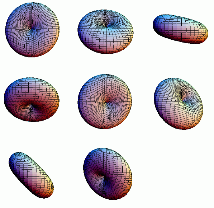
Figure 2: View of the magnetosphere at different rotational phases separated by $\pi/4$. For a full movie of the eclipse see http://www.physics.mcgill.ca/$\sim$lyutikov/movie.gif

The modulation of the radio flux during the eclipse is due to the fact that – at some rotational phases of pulsar B – the line of sight will only pass through open magnetic field lines where is assumed to be negligible. One of the main successes of the model is its ability to reproduce both the single and double periodicities of these transparent windows, at appropriate places in the eclipse. This requires that $\vec{\mu}_{B}$ be approximately – but not quite – orthogonal to ${\bf\Omega}_{B}$. To understand this result geometrically, consider Figs. 2-3. The rotation of $\vec{\mu}_{B}$ out of the plane of the sky brings the observer’s line of sight to within a small angle of the magnetic pole (in the favored geometry). The cross-sectional area of the absorbing plasma is maximized at this moment, and it projects an ellipsoidal shape on the sky. On the other hand, when $\vec{\mu}_{B}$ sits in the plane of the sky, the absorbing plasma fills a region bounded by a set of closed dipole field lines (Fig. 3). The shifting inclination of $\vec{\mu}_{B}$ through one half a rotation of pulsar B allows the line of sight to intersect this dipolar region once or twice. The proportions of the eclipse in which either periodicity is observed depend on the the impact parameter $z_{0}$ and the extent to which $\vec{\mu}_{B}$ is nearly – but not quite – orthogonal to ${\bf\Omega}_{B}$. A major success of the model is that it can reproduce the relative sequence and duration of these distinct periodicities.

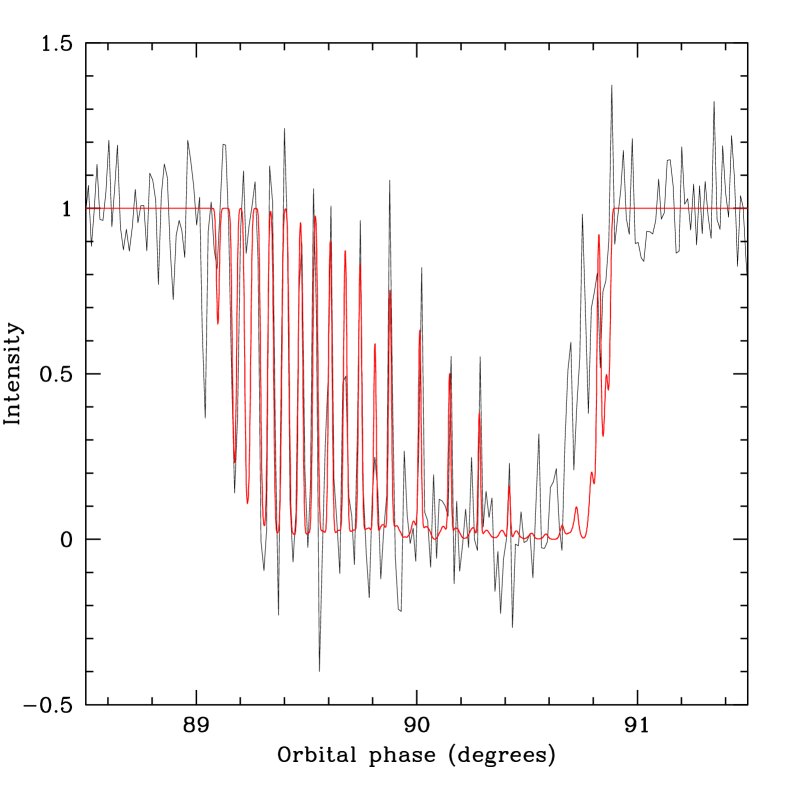
Figure 4: Comparison of a simulated eclipse profile (solid line) with 800 MHz data (McLaughlin et al., 2004). In the model, the absorbing electrons are distributed on the dipole magnetic field lines with a constant density $\lambda_{\rm mag}=3\times 10^{5}\,(k_{\rm B}T_{e}/10\,m_{e}c^{2})^{5/3}\,\nu_{\rm GHz}^{5/3}$ over a fixed range of radii $R_{\rm abs-}<R_{\rm max}<R_{\rm abs+}$. Here $R_{\rm abs+}=1.5\times 10^{9}$ cm and $R_{\rm abs-}=0.75R_{\rm abs+}$. The same light curve will result if $\nu$, $T_{e}$ and $\lambda_{\rm mag}$ varied jointly so as to keep $\lambda_{\rm mag}/(T_{e}\nu)^{5/3}$ fixed. The spin axis of pulsar B is oriented at $\theta_{\Omega}/({1\over 2}\pi)=0.66$ and $\phi_{\Omega}=-{1\over 2}\pi$. The inclination between ${\bf\Omega}_{B}$ and the magnetic moment $\vec{\mu}_{B}$ is $\chi/({1\over 2}\pi)=0.82$, and the impact parameter is $z_{0}=-7.5\times 10^{8}$ cm. The model light curve is smoothed over a timescale $\Delta t=0.25$ s with a gaussian window $e^{-\Delta\phi^{2}/2\sigma_{\phi}^{2}}$ [$\sigma_{\phi}=\Delta t/(2\pi)^{1/2}$]. The model fits the data best in the middle of the eclipse.

Our simulated light curve is displayed in Figs. 4 and 5. Variations in the parameters of the model modify the light curve in the following ways. A large asymmetry between ingress and egress results from a combination of finite $\theta_{\Omega}$ (inclination between the spin axis of pulsar B and the orbital plane normal) and finite $z_{0}$ (impact parameter). The asymmetry is largely erased if $\phi_{\Omega}$ is in the range $\pm 60^{\circ}$ (the rotation axis is out of the plane of the sky). There can be one or two transparent windows per rotation of pulsar B, depending on $z_{0}$ and $\chi$ (the angle between rotational angle and magnetic moment). If $\chi$ differs considerably from $\pi/2$, then both eclipse center and egress show strong modulation on a single rotational period. A very small value of $R_{\rm abs-}$ results in a complete eclipse in the center. Since $\nu\gtrsim\nu_{B,e}$ in most or all of the eclipse, the inner boundary corresponding to $\nu_{B,e}/\gamma_{\rm e}\nu>1$ is never reached.

Based on a sample of many eclipse light curves our best fit parameters are: $z_{0}\simeq-7.5\times 10^{8}$ cm, $\theta_{\Omega}\simeq 60^{\circ}$, $\phi_{\Omega}\simeq-90^{\circ}$, $\chi\simeq 75^{\circ}$. The orbital inclination is therefore predicted to be close to $90.55^{\circ}$. This is somewhat larger than that inferred by Cole et al. (2004) ($90.26^{\circ}\pm.13^{\circ}$), but consistent with the estimate of Ransom et al. (2004) ($88.7^{\circ}\pm.9^{\circ}$). Note that there is a symmetry in these parameters, $z_{0}\rightarrow-z_{0}$ and $\phi_{\Omega}\rightarrow-\phi_{\Omega}$, which preserves the shape of the light curve. In view of results of Cole et al. (2004), we have chosen $z_{0}<0$.

The dependence of the eclipse profile on the parameters $z_{0}$, $\theta_{\Omega}$ and $\chi$ is illustrated in Fig. 8. Overall the best constrained parameter is $z_{0}\sim-7.5\times 10^{8}$ cm, which must lie within a range a range $\sim\pm 10\,\%$ of this value. There is however, a degeneracy between $\theta_{\Omega}$ and $\chi$ which produces nearly identical light curves if both angles are varied up or down by the same factor. The results are not sensitive to $|\phi_{\Omega}+90^{\circ}|\lesssim 30^{\circ}$.

The required minimum multiplicity is $\lambda_{\rm mag}\simeq 3\times 10^{5}\,\nu_{\rm GHz}^{5/3}\,(k_{\rm B}T_{e}/10\,m_{e}c^{2})^{5/3}$ to reduce the transmitted radio flux by $\gtrsim 90\,\%$ at an orbital phase of $\sim 90.5^{\circ}$. This electron density is, in fact, close to the estimates (10) and (12). The full duration of eclipse is about $40$ sec. The size of the eclipsing region is $R_{\rm abs+}=1.5\times 10^{9}$ cm, so that the absorbing plasma must be truncated well inside the expected radius of the magnetopause. We comment on the significance of this result in the next section.

The model readily reproduces many fine details of the eclipses. It explains the modulation of that is observed at the first and second harmonics of the spin frequency of pulsar B, and the deepening of the eclipse after superior conjunction. The average eclipse duration is almost independent of frequency when the multiplicity is larger than $\lambda_{\rm mag}\sim 3\times 10^{5}$ (Fig. 6). Eclipse is broader when the magnetic moment of pulsar B is pointing closest to the observer, just as is observed (McLaughlin et al., 2004). Figure 7 shows the eclipse profile averaged over different orientations of magnetic moment. When $\vec{\mu}_{B}$ is pointing towards the observer the “doughnut” of the closed field lines is seen nearly face-on, producing broad eclipses; when $\vec{\mu}_{B}$ is in the plane of the sky the “doughnut” is seen edge-on, producing narrower eclipses.

It should also be noted that the details of eclipse ingress and egress are not fully reproduced by the model: in particular the rise in the radio flux at egress is sharper than observed (especially if $\lambda_{\rm mag}$ is high enough to give the eclipses a weak frequency dependence). This could be due to deviations of the actual magnetic field from our assumption of a pure dipole; or be an artifact of our assumption of a sharp plasma boundary. We examine the effects of a smoother plasma profile and a variable electron temperature profile in §6.

5.4 Eclipse Duration

Our eclipse calculations show that the optical depth of the absorbing plasma undergoes a sharp drop at a distance $R_{\rm abs+}\simeq 1.5\times 10^{9}$ cm from pulsar B. This is about $2.5$ times smaller than the expected radius of the magnetopause, $R_{\rm mag}\simeq 4\times 10^{10}$ cm (assuming that the torque parameter ${\cal N}_{B}$ is unity in eq. (4)). The disagreement with the maximum lateral extension of the closed field lines is closer to a factor of 4 (e.g. Lyutikov, 2004).

The synchrotron optical depth (52) reflects both the geometrical distribution of absorbing particles, and their temperature profile. One possibility is that $R_{\rm mag}$ has been overestimated, and that $R_{\rm abs+}$ reflects the actual boundary of the pulsar B magnetosphere. Alternatively, the suppression in $\tau_{\nu}$ could be due to particle loss and overheating in the outer magnetosphere. Let us consider these possibilities in turn (we clearly favor the latter).

Recall that the torque parameter ${\cal N}_{B}$ is presently unknown. The surface magnetic field of pulsar B could be smaller than is implied by the the simplest estimate of the spindown torque (${\cal N}_{B}\sim 1$; eq. (1)). The torque formula (1) assumes an increase in the opening of the dipole field lines that is expected from simple geometry. But other effects are at work. The pressure is distributed asymmetrically about pulsar B, so that even if its spin were in corotation with the orbit, it would be still be torqued by the pulsar A wind (the Magnus torque, e.g. Thompson et al., 1994; Arons et al., 2004). In addition, a strong surface resistivity at the interface between the pulsar B magnetosphere and the shocked wind of pulsar A would result in an enhanced spindown torque, due to the resistive dragging of the poloidal field lines of pulsar B.

There is a clear upper bound on the torque and spindown luminosity of pulsar B:

$$L_{B}\lesssim B_{\rm NS}^{2}R_{\rm NS}^{2}c\left({R_{\rm NS}\over R_{\rm mag}}\right)^{3}{\Omega_{B}R_{\rm NS}\over c}$$ (54)

which comes from the limit of comparable toroidal and poloidal fields at the magnetospheric boundary. Eq. (54) implies that ${\cal N}_{B}<c/(\Omega_{B}R_{\rm mag})\sim 10$. If ${\cal N}_{B}$ saturated this bound, the magnetospheric radius $R_{\rm mag}$ would be

$$R_{\rm mag}=\left({I_{B}\dot{\Omega}_{B}\over I_{A}\Omega_{A}\dot{\Omega}_{A}}\right)^{1/3}\left({cD_{AB}^{2}\over 2}\right)^{1/3}=2.4\times 10^{9}{\rm cm}$$ (55)

The lateral radius of the closed field lines is 50 percent larger, or $3.6\times 10^{9}$ cm, which is still a factor of 2 too large. Thus, one cannot explain small eclipse duration as being entirely due to large torque/small magnetic field of pulsar B.

The short eclipse duration may also reflect the loss of plasma from the outermost closed field lines, resulting from a change in the topology of the field lines. Experience with planetary magnetospheres suggests that the boundary between open and closed field lines can vary by a factor $\sim 1.5$ in polar angle (a factor $\sim 2$ in maximum dipole radius) from the windward side to the leeward side (e.g. Kabin et al., 2004). Indeed, the relativistic PIC simulations of Arons et al. (in preparation) show that the plasma is very dynamic in the vicinity of the separatrix between open and closed field lines.

If the magnetic field in the pulsar A wind alternates in sign over the pulsar A period (e.g. the wind is ‘striped’) then reconnection can occur over most of the magnetopause surface. On the other hand, if the direction of the wind magnetic field is constant in each rotational hemisphere of pulsar A, then reconnection will occur only on particular magnetospheric field lines that happen to run counter to the wind field. Trapped particles will, nonetheless, be effectively redistributed over the bulk of the magnetosphere by azimuthal drift. The drift timescale for particles of Lorentz factor $\gamma_{e}$ is $\sim R_{\rm mag}^{2}\nu_{B,e}(B_{\rm mag})/\gamma_{e}c^{2}\sim 2\times 10^{5}$ s, which is shorter than the residency time $\sim(\Omega_{B}f_{\rm cool})^{-1}\sim 5\times 10^{5}$ s (eq. [9]). As a result, the loss of particles by reconnection in the magnetotail would reduce the particle density on the windward side of the magnetosphere as well.

The loss of particles from the outer magnetosphere is likely to cause overheating of the remaining particles, which reduces the synchrotron absorption coefficient (5.1). A similar effect will occur if the trapped plasma has a large ion component, since the density (56) of the electron-ion plasma is suppressed in the outer magnetosphere. This variant of the eclipse model is examined in the following section.

Two other explanations for a short eclipse duration can be discounted. The angle between the line of sight and the orbital plane could be larger than is claimed by Cole et al. (2004) and Ransom et al. (2004). Increasing the inclination to $\sim 2^{\circ}$ would reduce the eclipse duration by a factor of two. However, our modeling of the eclipse profile places tight constraints on the orbital inclination which disfavor this possibility.

Another unlikely explanation for the narrow eclipse width is that the moment of inertia of pulsar B – but not of pulsar A (eq. [4]) – is much smaller than neutron star models suggest. More than an order of magnitude decrease in $I_{B}$ is required, which is not possible for (the lower mass) pulsar B even if it were composed entirely of $u$-$d$-$s$ symmetric quark matter.

6 Eclipses by an Ion-Supported Cloud

We now examine the case where the absorbing plasma is composed largely of electrons and ions. In this variant of the eclipse model, the plasma is more centrally concentrated around pulsar B than was assumed in §5; and allowance is made for a higher electron temperature in the outer magnetosphere.

The ions have two properties which influence the plasma distribution. First, they have a much stronger gravitational binding to the neutron star surface than do electrons and positrons; and, second, they cool much more slowly in the outer magnetosphere. These properties of the ions have opposing effects on the equilibrium electron density in the outer magnetosphere. On the one hand, the large gravitational binding energy makes it energetically favorable to force some of the slow-cooling electrons downward through the cooling radius (with a parallel electric field) if their temperature is $k_{\rm B}T_{e}\lesssim(A/Z)GM_{{\rm NS},B}m_{p}/R_{{\rm NS},B}\sim 200\,(A/Z)$ MeV. Here $Am_{p}$ is the ion mass, and $Ze$ its charge.

On the other hand, if the ions are themselves heated at the same time as the electrons, they will prevent the lighter charges cloud from collapsing through the cooling radius. The principal heating mechanisms which we examine in §4 involve the absorption of low-frequency transverse photons (radio waves). For example, heating of protons by such a mechanism will be suppressed if the proton cyclotron frequency $\omega_{B,p}=eB/m_{p}c$ sits below the plasma frequency of the (relativistic) electrons, $\omega_{P,e}=(2\pi n_{e}e^{2}c^{2}/k_{\rm B}T_{e})^{1/2}$. This gives a characteristic electron density

$$n_{e}=\left({k_{\rm B}T_{e}\over m_{p}c^{2}}\right)\,{B^{2}\over 2\pi m_{p}c^{2}}.$$ (56)

The corresponding lower bound on the multiplicity of the neutralizing electrons (mass $m_{e}$) is

$$\lambda_{\rm eq}^{e-i}={180\over\cos\theta_{B}}\,\left({k_{\rm B}T_{e}/m_{e}c^{2}\over 10}\right)\,\left[{(B_{\rm NS}R_{\rm NS}^{3})_{B}\over 5\times 10^{29}~{}{\rm G~{}cm^{3}}}\right]\,\left({r\over 4\times 10^{9}~{}{\rm cm}}\right)^{-3}.$$ (57)

This can be competitive with expression (10) somewhat inside the magnetopause, e.g. at $r\lesssim 1\times 10^{9}$ cm.

From the requirement that the electron pressure not exceed the magnetic dipole pressure and using electron multiplicity (57), the maximum temperature is

$${k_{\rm B}T_{e,\rm max}\over m_{e}c^{2}}={m_{p}\over 2m_{e}}\,\left(1+{T_{p}\over T_{e}}\right)^{-1/2}=9\times 10^{2}\,\left(1+{T_{p}\over T_{e}}\right)^{-1/2},$$ (58)

which applies as long as $k_{\rm B}T_{p}\lesssim m_{p}c^{2}$.

We therefore set the electron density to the threshold value for significant ion heating. Keeping in mind the results of §4.3, $n_{e}$ is fixed at a constant value (56)

$$n_{e}(R_{\rm max})=\left({k_{\rm B}T_{e}\over m_{p}c^{2}}\right)\,{B_{\rm mag}^{2}\over 2\pi m_{p}c^{2}}\,\left({R_{\rm max}\over R_{\rm mag}}\right)^{-6}$$ (59)

along each field line (labeled by the maximum radius $R_{\rm max}$). The corresponding multiplicity parameter $\lambda_{\rm eq}^{e-i}$ is given by eq. (57) or, equivalently, by

$$\lambda_{\rm mag}=\lambda_{\rm eq}^{e-i}(R_{\rm max})\,\left({R_{\rm max}\over R_{\rm mag}}\right)^{-3}.$$ (60)

The factor of $(R_{\rm max}/R_{\rm mag})^{-3}$ in this expression accounts for the normalization of the multiplicity $\lambda_{\rm mag}$ at the magnetospheric boundary $R_{\rm mag}$.

One also expects a very strong dependence of $T_{e}$ on $r$ when the electrons absorb the energy of large-scale torsional motions in the magnetosphere, and cool by incoherent synchrotron emission (SS4.2-4). The equilibrium temperature of the absorbing electrons is expected to increase rapidly with radius (eq. [30]). The synchrotron optical depth given by eqs. (5.1) and (50), with electron multiplicity (57), drops precipitously with distance from pulsar B,

$$\tau_{\nu}(r)\;\propto\;rn_{e}B^{2/3}(\nu T_{e})^{-5/3}\;\propto\;\varepsilon_{A}^{-4/9}\,\nu^{-5/3}\,r^{-97/9}.$$ (61)

(Here $\varepsilon_{A}$ is the energy density in torsional motions at radius $r$ in the pulsar B magnetosphere, relative to the magnetic pressure at the magnetopause boundary.) One finds, generically, a sharp transition from large to small optical depth, because of the much higher heating rates in the outer magnetosphere. Taking $\varepsilon_{A}$ to be constant gives the frequency scaling

$$\Delta\phi(\nu)\sim\nu^{-15/97}.$$ (62)

We therefore choose a temperature profile $T_{e}(r)\propto r^{7}$. After setting the magnetospheric radius to $R_{\rm mag}=4\times 10^{9}$ cm (${\cal N}_{B}=1$ in eq. [4]), the only free parameter in this model is the normalization of $T_{e}$, which is set to $k_{\rm B}T_{e}=10\,m_{e}c^{2}$ at $r=1.4\times 10^{9}$ cm. The resulting eclipse light curves are displayed in Fig. 9. One obtains an equally good fit to the central parts of the eclipse, and a smoother fall and rise in the radio flux at ingress and egress. The eclipse duration has a weak frequency dependence (Fig. 10), and the depth of the eclipse is less dependent on frequency than in the constant-$n_{e}$ model (compare Fig. 6).

A rapid increase in the temperature toward the edge of the magnetosphere (combined with a drop in $n_{e}$ to maintain pressure balance) can therefore provide an explanation for the duration of the observed eclipses. Indeed, the dependence of $T_{e}$ on $r$ could be even stronger than we assume if the amplitude $\varepsilon_{A}$ of the turbulence increases outward in the magnetosphere of pulsar B, and if there is enhanced plasma loss from the outer magnetosphere.

It should also be noted that our model of electron heating involves the absorption of low-frequency ($1-10$ MHz) radio waves (§4.2). This means that $\tau_{\nu}$ will maintain the scaling (61), and continue to drop off rapidly with radius, even when the plasma is optically thin at GHz frequencies.

7 Polarization

We now consider polarization effects associated with the propagation and absorption of the two electromagnetic modes in the eclipse region. In a magnetized, relativistic plasma these modes are linearly polarized below the synchrotron peak frequency, $\nu\lesssim\nu_{\rm peak}=\nu_{B,e}(k_{\rm B}T_{e}/m_{e}c^{2})^{2}$, even if the plasma is composed of electrons and ions (e.g. Sagiv et al., 2004). The linear absorption coefficients of the two modes are given by eq. (5.1). We present a sample calculation of the polarization of the transmitted radio pulses in our favored eclipse model, under the assumption that the incident radiation is unpolarized. In this case, the radiation can become polarized as it propagates through an absorbing medium.

In an inhomogeneous plasma (where the density and/or the magnetic field are functions of position), it is more convenient to describe radiation transfer in terms of modes polarized along fixed directions in space. We will choose these reference polarization states to lie along the normal to the orbital plane ($a$), and within the orbital plane ($b$). The radiation field is then characterized by four Stokes parameters $I$, $Q$, $U$ and $V$. The first two parameters can be re-expressed in terms of the intensities in the two reference polarization states, $I=I^{a}+I^{b}$ and $Q=I^{a}-I^{b}$. The polarization fraction is $\Pi=\sqrt{U^{2}+Q^{2}+V^{2}}/I$.

Our calculation of the transmitted polarization neglects the effects of synchrotron re-emission and Faraday rotation. The first effect can be safely neglected if one is interested in the pulsed component. Faraday rotation is absent in a pair plasma, while for electron-ion plasma at low frequencies it is suppressed by a factor $\sim\nu/\nu_{\rm peak}$ compared with the effects of synchrotron absorption. One consequence of this is that the effects of mode tracking are also negligible. This means that the instantaneous polarization angle, $\chi={1\over 2}\tan^{-1}(U/Q)$, is not able to adjust adiabatically to the changing direction of the magnetic field (e.g. Thompson et al., 1994).

Marginally, effects of limiting polarization may lead to generation of small circular polarization, which depends on the difference $n_{2}-n_{1}$ between the mode indices of refraction depends on the angle between $\hat{k}$ and ${\bf B}$. In a relativistic thermal plasma $n_{2}-n_{1}$ depends on the angle between $\hat{k}$ and ${\bf B}$; approximately

$$(n_{2}-n_{1}){\omega\over c}\;\simeq\;{\Gamma(1/3)\over 2^{2/3}\pi}\,\alpha_{\nu}\;=\;0.54\,\alpha_{\nu}\;\;\;\;\;\;\;\;\;\;\left[\nu\ll\nu_{B,e}\left(k_{\rm B}T_{e}/m_{e}c^{2}\right)^{2}\right],$$ (63)

where $\alpha_{\nu}$ is the polarization-averaged synchrotron absorption coefficient (e.g. Sagiv et al., 2004). In this situation, the most important consequence of this phase shift is to generate finite circular polarization. The circular polarization parameter $V$ turns out to be small, but we include it in the calculation for completeness.

Within the above approximations, the equations of polarization transfer read

$${dI^{a}\over dx} = -I^{a}\left[\alpha_{\nu}^{(1)}\sin^{4}\chi_{B}+\alpha_{\nu}^{(2)}\cos^{4}\chi_{B}+{1\over 2}\alpha_{\nu}\sin^{2}(2\chi_{B})\right]+{1\over 4}U\left[\alpha_{\nu}^{(1)}-\alpha_{\nu}^{(2)}\right]\sin(2\chi_{B})\mbox{}$$

$$-{1\over 2}V\left[{\omega\over c}(n_{2}-n_{1})\right]\sin(2\chi_{B});\mbox{}$$

$$\mbox{}{dI^{b}\over dx} = -I^{b}\left[\alpha_{\nu}^{(1)}\cos^{4}\chi_{B}+\alpha_{\nu}^{(2)}\sin^{4}\chi_{B}+{1\over 2}\alpha_{\nu}\sin^{2}(2\chi_{B})\right]+{1\over 4}U\left[\alpha_{\nu}^{(1)}-\alpha_{\nu}^{(2)}\right]\sin(2\chi_{B})\mbox{}$$

$$+{1\over 2}V\left[{\omega\over c}(n_{2}-n_{1})\right]\sin(2\chi_{B});\mbox{}$$

$$\mbox{}{dU\over dx} = -\alpha_{\nu}U+{1\over 2}(I^{a}+I^{b})\left[\alpha_{\nu}^{(1)}-\alpha_{\nu}^{(2)}\right]\,\sin(2\chi_{B})+V\left[{\omega\over c}(n_{2}-n_{1})\right]\cos(2\chi_{B});\mbox{}$$

$$\mbox{}{dV\over dx} = -\alpha_{\nu}V+\left[(I^{a}-I^{b})\sin(2\chi_{B})-U\cos(2\chi_{B})\right]{\omega\over c}(n_{2}-n_{1})$$ (64)

(e.g. Pacholczyk & Swihart, 1970). Here, $\chi_{B}$ is the angle between the reference direction $a$ and the projected magnetic field (at a certain point $x$ along the line of sight).

The Stokes parameters are plotted in Fig. 11 for our best fit eclipse model. The transmitted radiation is predicted to be strongly polarized in the deepest part of the eclipse, with a polarization fraction reaching $25\%$. (This is, unfortuntely, the time when the signal to noise ratio is smallest.) The polarization angle evolves smoothly throughout eclipse. One finds $U\lesssim Q$ when $\Pi$ is largest, which means that the transmitted polarization tends to be aligned with one of the two reference polarization directions. The main contribution to $U$ and $Q$ comes from regions of the magnetosphere which have finite transparency.

We find that the net value of $V$ is much smaller than that of $U$ and $Q$, by one or two orders of magnitude, in the case where the background source is unpolarized. This is partly the result of a cancellation between the ingoing and outgoing parts of the ray trajectory.

Polarization provides an independent test of the eclipse mechanism and the geometry of the system. The radio pulses of pulsar A are, in fact, strongly polarized (up to $50\%$: Ransom et al., 2004). In order to predict correctly the transmitted polarization, one needs to know the direction of polarization with respect to the orbital plane. This can be achieved using calibration of polarization angle, i.e. by referencing to a source with known position angle, and a determination of the orientation of the orbit on the sky (by combining the scintillation measurements with the anticipated proper motion measurements).

8 Predictions and Comparison with Other Models

8.1 Predictions of the model

We now summarize the predictions of our model, and how further observations can be used to probe the geometry of the system and the properties of the eclipsing material.

1. The impact parameter $z_{0}$ between the line of sight and the orbital plane is predicted to be $|z_{0}|=7.5\pm 0.7\times 10^{8}$ cm. The corresponding orbital inclination is $90.55^{\circ}\pm 0.05^{\circ}$ (or possibly $89.45^{\circ}\pm 0.05^{\circ}$). This prediction is intermediate between the measurements of Cole et al. (2004) and Ransom et al. (2004).

2. The spin ${\bf\Omega}_{B}$ of pulsar B is expected to undergo geodetic precession on a $\sim 75$ year timescale (Burgay et al., 2003). We have provided predictions for how the eclipse light curve will vary as a result. In particular, the orbital phase at which the radio flux reaches a minimum will shift back toward superior conjunction (Fig. 13). Since $\phi_{\Omega}$ is not well constrained, a time for eclipse to become symmetric is between $\sim$ 12 years (if $|\phi_{\Omega}+90^{\circ}|\sim 30^{\circ}$ and ${\bf\Omega}_{B}$ is drifting away from $\phi_{\Omega}=-90^{\circ}$) and $\sim$ 25 years (if $\phi_{\Omega}$ is drifting toward $-90^{\circ}$).

3. High time-resolution observations are a sensitive probe of the distribution of plasma properties (density and temperature) on the closed field lines. If plasma is depleted from the outermost field lines, at high temporal resolution the flux should return to unity. On the other hand, if the absorbing plasma does not have a sharp truncation in radius, then the flux will not return to unity in all of the transparent windows.

4. The eclipses must regain a strong frequency dependence at sufficiently high frequencies. The critical frequency above which significant transmission occurs can be used to place tight constraints on the plasma density. The electron cyclotron frequency at a distance $r\sim z_{0}\sim 7.5\times 10^{8}$ cm from pulsar B is estimated to be $\nu_{B,e}\sim 3$ GHz. One therefore expects the eclipses to develop a significant frequency dependence at higher frequencies.

5. There are a number of definite predictions for the polarization of the transmitted radiation as discussed in §7. The propagation of the radio waves through the intervening magnetosphere is in the quasi-transverse regime, where the polarization eigenmodes are linear and Faraday rotation can be neglected. The rotation measure should therefore not change significantly during the eclipse, and the variation in the dispersion measure is predicted to be small, of the order of $10^{13}$ cm^-2.

Finally, we note that the model predicts some radio emission from the magnetosphere of pulsar B, but its precise amplitude and spectrum cannot be easily determined from first principles. A straightforward upper bound to the radio output is obtained for incoherent synchrotron radiation. The luminosity of electrons (and positrons) radiating at temperature $T_{e}$ can be no larger than the blackbody at this temperature:

$${dL_{\rm bb}\over d\ln\nu}={2\pi k_{\rm B}T_{e}\nu^{3}\over c^{2}}(4\pi R_{\rm mag}^{2})=1\times 10^{22}\,\nu_{\rm GHz}^{3}\,\left({k_{\rm B}T_{e}/m_{e}c^{2}\over 10}\right)\,\left({R_{\rm mag}\over 4\times 10^{9}~{}{\rm cm}}\right)^{2}\;\;\;\;\;\;{\rm ergs~{}s^{-1}}.$$ (65)

This is too weak to be important, and so the emission must be of a coherent type such as we have described.

8.2 Alternative Eclipse Models

In this section we briefly contrast our favored eclipse model with other mechanisms. At first sight, an important clue is that the electron cyclotron frequency, measured along the line of sight, peaks at a value close to the observing frequency. Thus, it is tempting to associate the eclipses with absorption of the radio waves on non-relativistic particles. Indeed, we have outlined a mechanism for supplying a constant flux of non-relativistic electrons (and ions) on the closed magnetic field lines (in Appendix A). If the closed dipolar field lines of pulsar B are twisted through an angle $\Delta\phi\sim 1$ radian, then the optical depth through the cyclotron resonance (of either type of charge) is $\tau_{\rm cyc}\sim\beta_{\parallel}^{-1}$. Here $\beta_{\parallel}$ is the drift speed of the charges, in units of the speed of light. Thus, a sub-relativistic drift of the charges (e.g. with a speed $\beta_{\parallel}\sim\Omega r/c$) would guarantee a significant optical depth at the cyclotron resonance.

There are two difficulties with this very simple model. First, the duration of the eclipse has a weak frequency dependence. The eclipses extend out to a distance $R_{\perp}\simeq\pm 1.5\times 10^{9}$ cm from superior conjunction (in a direction parallel to the orbital plane). For example, if the magnetic moment of Pulsar B were directed toward the observer, then the maximum electron cyclotron frequency along the line of sight would be

$$\nu_{B,e}=400\;{\cal N}_{B}^{3/4}\left({z_{0}^{2}\over R_{\perp}^{2}}+1\right)^{-3/2}\;\;\;\;{\rm MHz}$$ (66)

at eclipse ingress (or egress). Here $z_{0}$ is the offset of the line of sight from the orbital plane. The inclination of the orbital plane with respect to the line of sight is ${\pi\over 2}-i$, where $i$ is the inclination with respect to the plane of the sky. One then has

$$z_{0}=\left(i-{\pi\over 2}\right)D_{AB}$$ (67)

The corresponding expression is

$$\nu_{B,e}=400\;{\cal N}_{B}^{3/4}\left({z_{0}^{2}\over R_{\perp}^{2}}+1\right)^{-2}\,\left({4z_{0}^{2}\over R_{\perp}^{2}}+1\right)^{1/2}\;\;\;\;{\rm MHz}$$ (68)

when the magnetic moment is oriented perpendicular to the orbital plane. Inverting these expressions, one obtains $R_{\perp}$ as a function of $\nu_{B,e}$ for a fixed impact parameter. In both cases, it is a stronger function of frequency than $R_{\perp}\sim\nu_{B,e}^{-1/3}$ when $b\neq 0$. In addition, one observes that absorption must occur at a harmonic $>1$ unless the torque parameter ${\cal N}_{B}>1$ (see eq. 4).

Cyclotron absorption inside the magnetosphere of pulsar B has some advantages: the cross section is larger than it is for synchrotron absorption by relativistic particles, and the required particle density is thereby reduced. To have an appreciable optical depth at a radius $r$ (and corresponding frequency $\nu_{B,e}(r)$) the particle density should exceed the local Goldreich-Julian density by a factor $(\Omega_{B}r/c)^{-1}\sim 10$. Second, the eclipse is observed to begin roughly where the line of sight passes deep enough into the magnetosphere of pulsar B that $\nu_{B,e}\sim\nu$. Cyclotron absorption is, nonetheless, strongly disfavored for at least two reasons: first the expected frequency dependence of the eclipse duration is $\Delta\phi\propto\nu^{-1/3}$ (or a stronger function of frequency), in contradiction with the much weaker observed scaling $\Delta\phi\propto\nu^{-0.1}$; and, second, the absorbing particles will inevitably be heated to relativistic temperatures. In addition, a fluctuating component of the current would cause a heavy fossil disk of cold particles, which could be centrifugally suspended in the outer magnetosphere, to be drained on a very short timescale (cf. Thompson et al., 2002).

Our favored plasma parameters differ substantially from those advocated by Rafikov & Goldreich (2004), basically because we invoke a much stronger heating mechanism, and a different source of relativistic particles. At high optical depth, particles are isotropized much more easily, and the equilibrium particle density regulates to a much larger value (due to the competition between injection from below and precipitation through the cyclotron cooling radius). If the external radio photons are the primary heat source, as advocated by Rafikov & Goldreich (2004), then the optical depth at the cyclotron fundamental is regulated to value of the order of unity. One infers that the eclipse duration should vary as $\Delta\phi\sim\nu^{-1/3}$ (or as a strong function of $\nu$ if the radio pump radiation is brighter at $\sim 100$ MHz than it is at $\sim 1$ GHz).

We have also considered effects of induced Compton scattering of pulsar A radio emission by plasma in pulsar B magnetosphere and by pulsar B radio beam (e.g. Thompson et al., 1994). Both effects are negligible due to a small optical depth.

9 Conclusion

We have developed a model of the radio eclipses of pulsar J0737$-$3039A, in which synchrotron absorption on relativistic particles occurs inside the intervening magnetosphere of the companion pulsar B. We believe that the value of such modeling is threefold. First, it provides a strong test of the longstanding assumption that isolated neutron stars are surrounded by corotating, dipolar magnetic fields. Second, one is probing how a pulsar magnetosphere interacts with an external wind, and in particular the mechanism by which turbulence is damped in a relativistic and magnetically dominated plasma. Third, an understanding of how charges are supplied to the magnetosphere may have broader implications for the electrodynamics of radio pulsars.

Given the simplicity of the model, it is in excellent agreement with observations, especially in the middle of the eclipse where the interaction with the external wind has only a modest effect on the shape of the poloidal field lines. The model can explain the asymmetry of the eclipse between ingress and egress; the weak frequency dependence of its duration; the modulation of the pulsar A emission at both the spin period of pulsar B, and half its spin period, in different parts of the eclipse; the detailed shape of the luminosity spikes in the middle of the eclipse; and the dependence of the eclipse duration on the rotational phase of pulsar B. The model implies that pulsar B is nearly, but not exactly, an orthogonal rotator. It also requires the spin axis of pulsar B to be tilted from the normal to the orbital plane.

We have demonstrated that – at intermediate distances – the poloidal magnetic field of a neutron star is well approximated by a dipole. This is a valuable confirmation of a fundamental assumption made in models of pulsar electrodynamics. In addition, our results are consistent with models that place the source of the radio emission close to the magnetic axis. Note that McLaughlin et al. (2004) define phases with respect to the arrival of radio pulses from pulsar B, whereas we define them with respect to the magnetic axis of B. On the other hand, the dependence of eclipse duration on pulsar B phase in our model is the same as inferred by McLaughlin et al. (2004), so that the two definitions of phases are close to each other.

In the present model we have neglected the fact that the radio pulse profile of pulsar B has a single peak. This can be used to put addition constraints on the geometry of the system, assuming that the radio emission mechanism is the same at both magnetic poles. In particular, in order for the radio beam from one of the pole to miss the observer, the angle $\phi_{\Omega}$ should not be equal to $\pm 90^{\circ}$. This comes from the fact that for $\phi_{\Omega}=\pm 90^{\circ}$ the angle between the direction of the magnetic moment and the line of sight is the same every half a period. Unfortunately, in the absence of pulsar radio emission model with predictive power, this does not provide any meaningful constraint at the moment.

Our eclipse model has implications for the formation and evolution of the PSR J0737$-$3039A system. The tilt of the spin axis of pulsar B with respect to the normal to the orbital plane is consistent with a large natal kick (as has been inferred from the spatial velocity of the system: Ransom et al. (2004)). The kick would change the orientation of the orbital plane and disrupt any pre-existing alignment between orbit and the spin of the progenitor star. Our measurement also does not support the suggestion of Demorest et al. (2004) that the spin axis should become aligned with normal to orbital plane due to torque from pulsar A.

We have also described how an optically thick, relativistic, thermal plasma may be maintained in the outer magnetosphere of pulsar B, where synchrotron cooling is slow. We have argued that the interaction between the wind of pulsar A and the magnetosphere is much more effective at heating the particles than is the absorption of the radio pulses of pulsar A. This interaction also generates two sources of particles on the closed magnetic field lines. First, bunches of relativistic charges are created by a pulsar-type mechanism close to the neutron star surface as the dipolar field lines are twisted back and forth close to the magnetic poles. Second, magnetic helicity builds up on the dipolar field lines, as the result of the asymmetry between the outgoing and return currents in each magnetic hemisphere. The resulting steady current supplies a constant flow of electrons and ions from the star to the outer magnetosphere.

The relativistic charges flowing in the magnetosphere of pulsar B are generally a more potent source of radio photons than is the companion pulsar. The requirement for this to be true is that the efficiency of conversion of turbulent energy to radio photons is larger than $\sim 10^{-7}$. (For example, if the unpulsed radio emission originates in the magnetosphere of pulsar B, then this minimal efficiency is exceed by $\sim 10^{4}$.) As a result, heating of the magnetospheric particles occurs mainly through self-absorption of these internally generated photons. Heating of ions can have an important regulatory effect on the equilibrium electron density: if $n_{e}$ exceeds a critical value, then radio photons that resonate with the ion gyromotion are absorbed by the plasma. A plausible source of low frequency pump photons has also been identified. This involves a two-step emission process: a cascade of torsional Alfvén waves to high frequencies where the waves become charge starved; followed by wiggler emission of radio waves by the electrostatically accelerated charges in the fluctuating magnetic field.

Appendix A Helicity Pumping on the Closed Magnetic Field Lines

The excitation of large-scale torsional motions provides a robust mechanism for drawing charges into the outer magnetosphere of pulsar B. Damping of this turbulence will also heat the suspended particles (§4.2), and if the heating rate is too high then the plasma may not absorb radio waves effectively. This leads us to examine a subtler effect, involving a static component of the magnetospheric twist, which will operate deeper in the magnetosphere of pulsar B where the fluctuating current is small, $|\delta J|\ll|\rho_{\rm GJ}|c$.

The exterior magnetic field of a neutron star can store a considerable amount of magnetic helicity. When it does, the current flowing nearly parallel to the magnetic field has a zero-frequency component. In the magnetically active Soft Gamma Repeaters and Anomalous X-ray Pulsars, the unwinding of a strong, internal magnetic field is a repeating source of magnetic helicity for the exterior of the star (Thompson et al., 2002). One does not expect such a mechanism to be active in the much older (and weakly magnetic) PSR J0737$-$3039.

Nonetheless, we offer a simple argument why magnetic helicity will be pumped from the outer to the inner magnetosphere of pulsar B. There are two simple components to this argument. First, if a fixed amount of helicity is injected into a dipole magnetic field, then the energy in the toroidal magnetic field is minimized if the helicity

$${\cal H}\sim(\pi r^{2})^{2}B_{P}B_{\phi}\sim(\pi B_{P}r^{2})^{2}\Delta\phi$$ (A1)

is concentrated close to the star (Thompson et al., 2002). Here $B_{P}$ is the poloidal magnetic field at radius $r$, and $B_{\phi}\sim B_{P}\Delta\phi$. The energy in the toroidal magnetic field is

$$E_{\phi}\sim{1\over 12}B_{\phi}^{2}r^{3}\sim{{\cal H}^{2}\over 12\pi^{2}r^{5}B_{P}^{2}}\propto{\cal H}^{2}r.$$ (A2)

If a magnetosphere carrying helicity ${\cal H}$ is not in the minimum energy state, the winding of the magnetic field can be rapidly transferred by reconnection between different flux surfaces (e.g. Taylor 1974).

The second observation is that the current flowing out along an open bundle of magnetic field lines will not be compensated precisely by the return current in the same magnetic hemisphere. There is, as a result, a residual current connecting the two magnetic poles, which flows along the outermost closed magnetic field lines. This closed field current imparts a small amount of helicity to the magnetosphere. By the above argument, this helicity will be pumped, by reconnection, on a short timescale $\sim c/\Omega$ to the inner magnetosphere. The net rate of transfer of helicity is then

$${d{\cal H}\over dt}\biggr{|}_{+}\sim\varepsilon_{\cal H}\Phi_{\rm open}^{2}\Omega.$$ (A3)

Here $\Phi_{\rm open}$ is the magnetic flux $\Phi(r)=\pi B_{P}(r)r^{2}$ evaluated at the boundary radius of the magnetosphere.

In the case of an isolated neutron star, an imbalance between the outgoing and return current can result from an offset $\Delta R_{\rm dipole}$ of the magnetic dipole from the center of the star. One then deduces

$$\varepsilon_{\cal H}\sim{\Omega\Delta R_{\rm dipole}\over c}<{\Omega R_{\rm NS}\over c}.$$ (A4)

Making use of $\Phi_{\rm open}=\pi B_{\rm pole}R_{\rm NS}^{2}(\Omega R_{\rm NS}/c)$, one can relate the helicity increase (A3) to the magnetic dipole luminosity $L_{\rm MDR}={1\over 6}(\Omega R_{\rm NS}/c)^{4}B_{\rm pole}^{2}R_{\rm NS}^{2}c$,

$${d{\cal H}\over dt}\biggr{|}_{+}\sim 6\pi^{2}L_{\rm MDR}\Delta R_{\rm dipole}.$$ (A5)

where $B_{\rm pole}$ is magnetic field at the magnetic pole of the star.

The effect is much stronger in the case of PSR J0737$-$3039B. The strong asymmetry in the external stress of the pulsar A wind will enforce a large asymmetry between the outgoing and return currents in each magnetic hemisphere. We therefore estimate

$$\varepsilon_{\cal H}\sim\Delta\phi(R_{\rm mag})\sim{\Omega_{B}R_{\rm mag}\over c}\sim 0.1-0.2.$$ (A6)

The equilibrium twist angle that is established at smaller radii depends on how rapidly the helicity is damped in the inner magnetosphere. We will not examine this problem here, and simply note that the inward flux of helicity allows one to establish a minimal static twist angle $\Delta\phi$ in the outer parts of the magnetosphere. Given that the twist is transferred between flux surfaces with a speed $\sim c$, one has

$${d{\cal H}\over dt}\biggr{|}_{+}\sim\Phi^{2}(r)\,\Delta\phi(r)\,{c\over r}.$$ (A7)

Combining this with eqs. (A3) and (A6) gives

$$\Delta\phi(r)\sim\left({\Omega_{B}R_{\rm mag}\over c}\right)\,\left({r\over R_{\rm mag}}\right)^{3}.$$ (A8)

The corresponding current is

$${J\over|\rho_{\rm GJ}|c}\sim 3\,\left({\cos\theta_{B}\over 0.3}\right)^{-1}\,\left({r\over R_{\rm mag}}\right)^{2}.$$ (A9)

It will be noted that the presence of a zero-frequency component of the current will influence the non-linear couplings between torsional waves in the magnetosphere (Goldreich & Sridhar, 1997; Thompson & Blaes, 1998).

Figure 1: Geometry of the model. The absorbing plasma is axisymmetrically distributed about pulsar B, and extends as far as a distance $R_{\rm abs+}\leq R_{\rm mag}$ from the neutron star. The spin axis of pulsar B is defined by angles $\theta_{\Omega}$ and $\phi_{\Omega}$. The magnetic moment $\vec{\mu}_{B}$ makes angle $\chi$ with the spin axis and rotates around ${\bf\Omega}_{B}$ every 2.77 s, as the pulsar is carried by the orbital motion in the $y$-direction. The line of sight passes at distance $z_{0}$ above the orbital plane.

Figure 3: Inferred geometry of the pulsar B magnetosphere projected onto the $z-y$ plane at the two particular moments where $\vec{\mu}_{B}$ lies in the $z-y$ plane. The spin axis ${\bf\Omega}_{B}$ is inclined by angle $\sim 60^{\circ}$ to the $z$ axis and lies in the $y-z$ plane. The magnetic moment ${\bf\mu}_{B}$ makes an angle $\sim 75^{\circ}$ with ${\bf\Omega}_{B}$. Apparent velocity of pulsar ${\bf V}_{B}$ is along $-y$ axis. The line of sight passes at $z_{0}/R_{\rm abs+}\sim-0.5$. The absorbing plasma is located between the two drawn magnetic surfaces with $R_{\rm abs-}=.75R_{\rm abs+}<R<R_{\rm abs+}$. The inner circle marks the cooling radius $R_{\rm cool}=.05R_{\rm abs+}$. The dotted line is the equatorial plane, orthogonal to ${\bf\Omega}_{B}$. The two directions of ${\bf\mu}_{B}$ plotted correspond to pulsar B phases separated by half a period. Points corresponding to negative values of $y$ enter the line of sight first. The transition to one transparent window per rotation occurs near the point when the line of sight crosses the dashed field lines. A full eclipse occurs when the line of sight crosses both solid and dashed field lines.

Figure 5: Same as Fig. 4, but model and data side by side.

Figure 6: Frequency dependence of the eclipse profile, smoothed on a timescale $\Delta t=2.77$ s. Parameters are the same as in Fig. 4. At high frequencies eclipse duration should become strongly frequency-dependent. This can be used to place tighter constraints on plasma density.

Figure 7: Average eclipse profiles for different orientations of magnetic moment of B. Solid line: eclipse profile averaged over points $315^{\circ}<\phi_{B}<45^{\circ}$ and $135^{\circ}<\phi_{B}<225^{\circ}$, where $\phi_{B}$ is a rotational phase of B ($\phi_{B}\sim 0^{\circ},\,180^{\circ}$ corresponds to magnetic moment pointing nearly towards an obsever, while $\phi_{B}\sim 90^{\circ},\,270^{\circ}$ corresponds to magnetic moment in the plane of the sky). Dotted line: eclipse profile averaged over $45^{\circ}<\phi_{B}<135^{\circ}$, dashed line: eclipse profile averaged over $225^{\circ}<\phi_{B}<315^{\circ}$. Eclipse is broader when the pulsar is “face-on”. Parameters are the same as in Fig. 4.

Figure 8: Change in the eclipse light curve due to a variation in the impact parameter $z_{0}$ and the inclination $\chi$ between the magnetic and spin axes of pulsar B. Parameters are as in Fig. 4.

Figure 9: Comparison of a simulated eclipse profile with 800 MHz data (McLaughlin et al., 2004) in the model with large ion content (§6). The density depends on radius according to Eq. (57), and the temperature distribution is $k_{\rm B}T_{e}=10\,m_{e}c^{2}\,\nu_{\rm GHz}^{-1}\,(r/1.4\times 10^{9}~{}{\rm cm})^{7}$. The magnetospheric radius is $R_{\rm mag}=4\times 10^{9}$ cm (${\cal N}_{B}=1$ in eq. [4]). The other parameters $z_{0}$, ${\bf\Omega}_{B}$, and $\chi$ are the same as in Fig. 5. The model light curve is smoothed over $\Delta t=0.25$ s.

Figure 10: Frequency dependence of the eclipse profile in the model of Fig. 9, smoothed on a timescale $\Delta t=2.77$ s. Parameters are the same as in Fig. 9

Figure 11: Polarization generated during the eclipse of an unpolarized background source, in the model of Fig. 4. The reference directions for the linear polarization are the normal to the orbital plane ($a$); and the orbital plane ($b$). Only negligible circular polarization is produced ($V\simeq 0$).

Figure 12: (a) Predicted eclipse profile at high temporal resolution of $\Delta t=0.01$ s at 800 MHz. Parameters as in Fig. 4. The absorbing plasma has a sharp cutoff on dipole field lines extending beyond $R_{\rm abs+}=1.5\times 10^{9}$. In the transparent windows, the flux returns to the unabsorbed level. (b) Eclipse model with electron density given by eq. (56). Parameters as in Fig. 9. In some transparent windows, the flux is partially absorbed.

Figure 13: Prediction of the effects of geodetic precession on the eclipse light curve. The parameters are the same as in Fig. 9, but with a temporal resolution of $\Delta t=0.01$ sec.

References

- Arons et al. (2004) Arons, J., Backer, D. C., Spitkovsky, A., & Kaspi, V. M. 2004, astro-ph/0404159
- Burgay et al. (2003) Burgay, M., D’Amico, N., Possenti, A., et al. 2003, Nature, 426, 531
- Cole et al. (2004) Coles, W. A., McLaughlin, M. A., Rickett, B. J., Lyne, A. G., & Bhat, N. D. R. 2004, astro-ph/0409204
- Demorest et al. (2004) Demorest, P., Ramachandran, R., Backer, D. C., Ransom, S. M., Kaspi, V., Arons, J., Spitkovsky, A. 2004, ApJ, 615, 137
- Fung & Kuijpers (2004) Fung, P. K., & Kuijpers, J. 2004, A&A, 422, 817
- Goldreich & Julian (1969) Goldreich, P., & Julian, W. H. 1969, ApJ, 157, 869
- Harding et al. (2002) Harding, A. K., Muslimov, A. G., & Zhang, B. 2002, ApJ, 576, 366
- Goldreich & Sridhar (1997) Goldreich, P. & Sridhar, S. 1997, ApJ, 485, 680
- Hibschman & Arons (2001) Hibschman, J. A. & Arons, J. 2001, ApJ, 560, 871
- Holloway (1977) Holloway, N. J. 1977, MNRAS, 181, 9
- Kabin et al. (2004) Kabin, K. et al., 2004, Journal of Geophysical Research (Space Physics), A18, 5222
- Kaspi et al. (2004) Kaspi, V. M., Ransom, S. M., Backer, D. C., Ramachandran, R., Demorest, P., Arons, J., & Spitkovskty, A. 2004, ApJ, 613, 137
- Lyne et al. (2004) Lyne, A. G., et al. 2004, Science, 303, 1153
- Lyutikov (2004) Lyutikov, M. 2004, MNRAS, 353, 1095
- Lyutikov et al. (1998) Lyutikov, M. and Blandford, R. D. and Machabeli, G., 1999, MNRAS, 305, 338
- McLaughlin et al. (2004) McLaughlin, M. A., et al. 2004, ApJ, 616, 131
- Michel (1969) Michel, F. C., ApJ, 158, 727
- Pacholczyk & Swihart (1970) Pacholczyk, A. G. & Swihart, T. L. 1970, ApJ, 161, 415 Fransisco
- Rafikov & Goldreich (2004) Rafikov R. R. & Goldreich, P. 2004, astro-ph/0412355
- Ransom et al. (2004) Ransom, S. M., Kaspi, V. M., Ramachandran, R., Demorest, P., Backer, D. C., Pfahl, E. D., Ghigo, F. D., & Kaplan, D. L. 2004, ApJ, 609, 71
- Rybicki & Lightman (1979) Rybicki, G. & Lightman, A. P. 1979, Radiative Processes in Astrophysics, Wiley, New York
- Sagiv et al. (2004) Sagiv, A., Waxman, E., & Loeb, A. 2004, ApJ, 615, 366
- Taylor (1974) Taylor, J. B. 1974, Phys. Rev. Lett., 33, 1139
- Thompson et al. (1994) Thompson, C., Blandford, R. D., Evans, C. R., & Phinney, E. S. 1994, ApJ, 422, 304
- Thompson & Blaes (1998) Thompson, C. & Blaes, O. 1998, Phys. Rev. D, 57, 3219
- Thompson et al. (2002) Thompson, C., Lyutikov, M., Kulkarni, S. R. 2002, ApJ, 574, 332