Overview of Technical Approaches to RFI Mitigation

Abstract

This overview provides an interface between lines of thought on rfi mitigation in the fields of radio astronomy and signal processing. The goal is to explore the commonality of different approaches to help researchers in both fields interpret each others’ concepts and jargon. The paper elaborates on the astronomers’ concept of gain closure relations and how they may be used in a “self-calibrating” system of rfi cancellation. Further discussion of the eigen decomposition method in terms of rfi power and antenna gains introduces adaptive nulling and rfi cancellation through matrix partitioning. While multipath scattering appears at first glance to be fatal to methods of rfi cancellation, its effect is easily incorporated in frequency dependent gain coefficients under many circumstances.

Briggs & Kocz Overview of RFI mitigation techniques F.H. Briggs, Research School of Astronomy & Astrophysics, Mount Stromlo Observatory, Cotter Road, Weston, ACT 2611, Australia (fbriggs@mso.anu.edu.au)

1 Introduction

Astronomers are designing the next generation radio telescopes with the capabilities to solve many current puzzles about the origin of the planets, stars, galaxies and Universe itself. Since the telescope designs are one to two orders of magnitude more powerful than the best present telescopes, astronomers know that the new instruments are capable of making discoveries that will open whole new fields of research. New telescopes will not just solve old problems, but will certainly do unexpected things that have been impossible in the past.

The same advances in technology that make new radio astronomy possible are closely linked to the advances in telecommunications that are beginning to saturate the radio spectrum. Any new radio telescope will have additional layers of signal processing built in from the design stages that are intended to enable it to see through the background radio interference as well as possible. In this regard, modern technical solutions offer great hope, but in reality they are complex and expensive, and the resources (in terms of time and money) will probably not exist to allow radio astronomers to apply these methods effectively enough to keep up with the rising earth-generated radio background unless there is active coordination with the telecommunications industry.

Communications signals are fully polarized, coherent emission from carefully modulated currents in the broadcasting antennas; a communications signal is broadcast to provide maximum efficiency in use of a limited portion of the radio spectrum defined by its allocated bandwidth $BW$. The astronomical signals originate mainly in the incoherent emissions from huge clouds of faintly emitting atoms, molecules or energetic electrons whose “astronomical intensity” is a collective effect arising from their large numbers. The radiated powers are added incoherently, except in a few cases, such as the coherent addition of radiated electric field in the ionospheres of pulsars, Jupiter’s ionosphere, the active regions of the Sun or celestial masers. Astronomical signals in general are well represented by stochastic or gaussian noise.

Telecommunication reception requires decoding the fluctuations in the electric field of the signal, so that the field at each time step $T$ (where $T\approx 1/BW$) reliably carries information. The information that astronomers extract from their signals has a more statistical character, such as total intensity of the power per unit bandwidth (called flux density) of an astronomical source, along with other more detailed statistical measures such as the net polarization of the signal power and the variation of the flux density as functions of frequency and time. For the large variety of celestial sources that fall in the class called ‘continuum sources,’ which radiate a smooth spectrum over a wide range of frequencies, more power can be received from the source by simply increasing the bandwidth of the observation.

Astronomers have not generally been interested in measuring the electric field strength as a function of time, although this is likely to change for some astronomical applications, such as rapidly time-variable phenomena (for example: pulsars, transient bursts, signals from energetic particles impinging on the upper atmosphere [Huege & Falcke 2003, Suprun et al 2003]), especially with the more sensitive telescopes being planned for the future. The need for RFI mitigation has also increased astronomers’ awareness of the need for processing their E-field signals in real-time at full bandwidth, which is much more demanding and expensive than their historical procedures ([Barnbaum & Bradley 1998]).

While there do exist frequency bands that have been reserved for astronomy, receivers have become so sensitive that low level spurious harmonics and weak leakage from communication and navigation services are strong enough to corrupt and confuse the astronomical signals. Furthermore, pursuing answers to scientific questions drives astronomers to observe outside of the reserved bands. For example, neutral atomic hydrogen has a well known radiative transition at rest frequency $f_{o}$$\>=\>$$1420.4057$ MHz, for which there is a reserved astronomy band. However, astronomers now wish to trace the evolution of hydrogen in galaxies over cosmic time, and since observing galaxies at redshift $z\approx 1$ would correspond to looking back in time to when the universe was less than half its current age, radio astronomers pursue the hydrogen line to frequencies of $f=f_{o}/(1+z)\approx 700$ MHz or lower, where the radio spectrum is already in heavy use.

Astronomers have had great success in achieving high angular resolution and high dynamic range imaging. The question naturally arises, “why not simply image the rfi sources along with the celestial ones?” Under some circumstances, this is a successful approach (e.g. [Perley et al 2004]); however, the character of many RFI signals – variability, non-gaussianity – may not be compatible with the necessary conditions for obtaining sufficiently high-dynamic range aperture synthesis.

As in all of radio science, improvements in instrumentation and signal processing are providing the tools for performing astronomical observations in radio rich environments. These include:

1. Robust receivers Modern receivers benefit from linearity over a large dynamic range to avoid generation of spurious signals through intermodulation within the receiving system. Since astronomical signals are noise-like, astronomers have historically processed their signals with custom built correlators that operate at 1 or 2 bit precision, at the cost of adding a modest percentage of quantization noise. Newer telescopes that will operate in populated areas are designed to process data with 10 to 14 bits of precision, a cost only now affordable due to advances in low-cost digital processing electronics.

2. Sophisticated signal recognition and blanking mechanisms. Historically, this was performed in the post-detection domain, where it was labor intensive and called “data editing.” If done early in the receiving system chain, blanking can ease the large dynamic range requirements of the receiver backend (reducing the required bits of precision for example). It is always a concern that a process so violently non-linear as blanking may preclude the application of some classes of rfi cancellation for which linear systems are a prerequisite. These topics in rfi mitigationnhave been reviewed by Fridman and Baan ([Fridman & Baan 2001]) and are addressed by several papers at this conference.

3. RFI cancellation A number of recent papers have begun to explore methods of rfi cancellation and subtraction([Barnbaum & Bradley 1998, Ellingson et al 2001, Leshem et al 2000, Briggs et al 2000]). The series of papers by Leshem, van der Veen, Boonstra and colleagues have been especially important in applying the techniques of signal processing in the radio astronomical context (see [Boonstra et al 2004] in these proceedings for complete references).

The bulk of this paper forms a mini-tutorial covering several issues in rfi cancellation that were sources of confusion to the authors and their colleagues. The goal is to ease the transfer of technology between the astronomical and signal processing communities.

Of course, the best starting place for radio astronomy continues to be siting telescopes in radio quiet environments, and astronomy will always rely on good will and cooperation with radio-active spectrum users for communication and navigation services.

2 Radio Astronomical Arrays

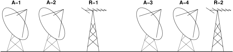
Figure 1: Astronomical telescope arrays with (1) conventional dish antennas pointed toward celestial radio sources and (2) reference antennas to provide increased gain in the direction of known interfering signals.

Modern radio telescopes operate in arrays in order to economically obtain sensitivity and angular resolution through the combination of the signal from the elements of the array (Figure 1). The radio astronomical convention is to denote antenna separations by a vector quantity $\overrightarrow{B_{ij}}$, indicating the relative positions of the antenna phase centers for antennas $i$ and $j$. These “interferometer baselines” are conveniently measured in wavelengths $\overrightarrow{B_{\lambda}}$ for which the effective angular resolution of each interferometer pair in the array is $\theta_{ij}=1/B_{\lambda,ij}$ radians. Definition of a cartesian coordinate system ($u$-$v$-$w$) with its $w$ axis pointing in the direction of a radio source allows $\overrightarrow{B_{\lambda}}$ to be specified by its components $u=B_{\lambda,u}$, $v=B_{\lambda,v}$, and $w=B_{\lambda,w}$. An array of elements at fixed locations will experience systematic variation of $u$, $v$ and $w$ as the Earth rotates. The $w$ component specifies the relative propagation delay between two elements of the array $t_{ij}=w_{ij}\lambda/c$, while the $u$ and $v$ components appear in the key equation of aperture synthesis,

$$V(u,v)=\frac{2k}{\lambda^{2}}\int p_{B}(x,y)T_{b}(x,y)e^{i2\pi(ux+vy)}dx\>dy$$ (1)

relating the “fringe visibility” $V(u_{ij},v_{ij})$ sensed by each interferometer pair $i,j$ in response to the angular brightness temperature distribution of the sky $T_{b}(x,y)$ modulated by $p_{B}(x,y)$, the primary beam gain function of the array elements. The strength and phase of the complex visibility result from the fourier integral of $p_{B}(x,y)T_{b}(x,y)$ over the celestial source. Here, $k$ is the Boltzmann constant, and $x$ and $y$ are angular coordinates measured in the plane of the sky. While this integral and its inversion form the essence of the aperture synthesis technique, a full description of the method requires entire books (e.g. [Thompson et al 1986, Taylor et al 1999]).

Interferometer arrays measure a $V_{m}(u,v)$ for each baseline through the cross correlation $C_{ij}$ of the signals $s_{i}$ and $s_{j}$ from two elements:

$$\hskip 42.67912ptV_{m}(u_{ij},v_{ij}) = <g_{i}s_{i}g_{j}^{*}s_{j}^{*}>$$

$$= C_{ij}$$

The signals entering the correlator have been scaled by the complex gain factors $g_{i}$ that quantify the differences in the signal paths from one array element to the next, and $*$ indicates complex conjugation. In general, $V_{m}(u,v,f)$, $g_{i}(f)$ and $s_{i}(f)$ are functions of frequency, and $C_{ij}(f)$ is the observed cross power spectrum. Provided the gains are constant over the integration time of the cross correlation product in Eqn. 2, the expression becomes $V_{ij}=V_{m}(u_{ij},v_{ij})=g_{i}g_{j}^{*}<s_{i}s_{j}^{*}>$.

3 Gain closure

The concept of “closure relations” becomes clear when combinations of observed correlation products are formed:

$$\hskip 5.69046ptQ=\frac{V_{ij}V_{kn}}{V_{in}V_{kj}} = \frac{g_{i}g_{j}^{*}<s_{i}s_{j}^{*}>g_{k}g_{n}^{*}<s_{k}s_{n}^{*}>}{g_{i}g_{n}^{*}<s_{i}s_{n}^{*}>g_{k}g_{j}^{*}<s_{k}s_{j}^{*}>}$$ (3)

$$= \frac{C_{ij}C_{kn}}{C_{in}C_{kj}}$$

The quantity $Q$ is a ratio of true visibilities for the radio source, regardless of whether the individual complex gains $g_{i}$ are known accurately or not.

The special case of an unresolved point source is of interest, since substituting a $\delta$-function for $T_{b}(0,0)$ in Eqn. 1 yields a visibility function that is constant for all $u,v$, implying that $Q=1$ and the $<s_{i}s_{j}^{*}>$ are equal for all $i,j$, so that the right hand side of the equation reduces to an identity relation among the gain coefficients.

The gain closure relations form the motivation for approaches to rfi mitigation since rfi sources can be treated as point sources and the cross correlations between rfi reference antennas and the astronomical signals provide the necessary information for computing the rfi contamination without precise knowledge of the gains of the element sidelobes through which the rfi enters the telescopes. These methods are in essence “self-calibrating.”

4 Cancellation

Most rfi cancellation schemes involve first identifying the interferer, followed by deducing the strength of its contamination within the astronomical data stream, and finally, precise subtraction of interferer’s contribution.

Fig. 2 illustrates one example of how that might be accomplished using the signal $I$ from an rfi reference antenna that is cross correlated with the astronomical signal $S_{A}$ in order to deduce the inter-coupling of the two signal paths. Several variations of implementing this scheme through the gain closure relations of cross power spectra were explored by [Briggs et al 2000]. Other schemes are implemented in the time domain (e.g. [Barnbaum & Bradley 1998, Kesteven et al, 2004]).

Separate rfi reference antennas serve two purposes: (1) They improve the signal-to-noise ratio on the interfering signal, in order to minimize the addition of noise to the astronomical observation during the application of rfi subtraction, and (2) with increased gain toward the interferer but decreased gain toward the celestial source, they avoid inadvertent subtraction of the astronomical signal along with the interference. It is important that the interference-to-noise ratio be better in the reference channel than the astronomy channels ([Briggs et al 2000]), but this is generally true since rfi enters the astronomy telescopes through weak sidelobes (roughly at the level of an isotropic antenna $\sim$0 dBi), while simple reference antennas can deliver 10 dB or more gain).

The gain information contained in the cross power spectrum $C_{AR}(f)$ between $(g_{A}S_{A}+g_{AI}I)$ and $g_{RI}I$ allows the rfi contamination of the voltage spectrum $g_{AI}I(f)$ in the astronomical data stream to be estimated from the reference voltage spectrum $g_{RI}I$:

$$\hskip 42.67912ptg_{AI}I = \frac{C_{AR}}{g_{RI}^{*}I^{*}}=\frac{g_{AI}g_{RI}^{*}II^{*}}{g_{RI}^{*}I^{*}}$$ (4)

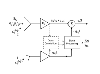
Figure 2: Example of interference cancellation scheme. In this case, there are two signal paths: (1) the astronomical signal $S_{A}$ entering the main antenna but corrupted by interference $I$, and (2) a reference antenna to pick up the interfering signal apart from $S$. The goal is for the signal processing to obtain a suitable signal for subtraction from the astronomical signal path to leave only an undistorted $S$. Techniques discussed here use cross correlation between Paths A and R to determine the filter coefficients.

Astronomers commonly measure the power spectrum of the signal from the telescope $P_{A}(f)$, which will have both power from the celestial source and rfi components $P_{A}(f)=|g_{A}S_{A}|^{2}+|g_{AI}I|^{2}$. In this case, an appropriate correction is preferably derived from two reference antennas labeled R1 and R2:

$$\hskip 36.98866pt|g_{AI}I|^{2} = \frac{C_{AR1}C_{AR2}^{*}}{C_{R1R2}^{*}}$$

$$= \frac{g_{AI}g_{R1}^{*}|I|^{2}g_{AI}^{*}g_{R2}|I|^{2}}{g_{R1}^{*}g_{R2}|I|^{2}}$$

The preference for dual reference signals arises from the nature of the noise in the cross power spectrum in the denominator of Eqn. 4; the noise term $<$$N_{R1}N_{R2}^{*}$$>$$(f)$ is a complex cross power spectrum that averages toward zero as integration time increases, unlike the noise $<$$|N_{R1}|^{2}$$>$$(f)$, which is real and positive and which would bias the result of Eqn. 4 if it were based on a single reference signal. When the subtraction is performed after the calculation of power spectra in this way, it is often described as “post-correlation” cancellation.

Similar estimation for the contamination of the $V_{m}(u,v)$ measurement of an interferometer pair $i,j$ of an array (Fig. 1) is

$$\hskip 28.45274ptg_{AiI}g_{AjI}|I|^{2} = \frac{C_{AiR1}C_{AjR2}^{*}}{C_{R1R2}^{*}}$$

$$= \frac{g_{AiI}g_{R1}^{*}|I|^{2}g_{AjI}^{*}g_{R2}|I|^{2}}{g_{R1}^{*}g_{R2}|I|^{2}}$$

with dual reference antennae.

Figure 3 gives an example of applying the relations in Eqn. 4. These Parkes observations covered a 64 MHz band centered on 676 MHz with 16384 spectral channels (3.9 kHz resolution). The goal of the program is the observation of neutral hydrogen clouds at reshift $z\sim 1$ in absorption against high $z$ radio galaxies. Two yagi reference antennas were oriented to point at the broadcasting tower for digital TV station channel 46 (652–659 MHz). The cancellation algorithm was applied to $\sim$0.1 sec integrations, followed by averaging for the full 16 sec scan. After cancellation of the digital TV, the noise level and weaker rfi contamination remains at the same level as the surrounding frequency bands; only those interferers in the yagi reception pattern have been canceled. ([Kesteven et al, 2004] give more details on the nature of the digital TV interference in their discussion of a real-time adaptive canceler.)

Figure 4 provides a closer look at the band containing the digital TV as a function of time through the 16 second scan – both before and after cancellation of the rfi signal. The noise level should be compared to that in a relatively “clean” band away from the TV (in the top panel of the figure). The clean band also contains an image of the peculiar drifting interferer, one of whose harmonics appears to the left of the TV band in panels B and C. The weak rfi spikes that remain throughout the spectrum (1) are narrower than the expected HI signals, (2) appear as emission features rather than absorption lines, and (3) take up a minor fraction of the spectrum as evidenced by the broad expanses between the narrow lines. This is encouraging for the success of redshifted HI studies.

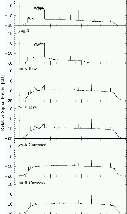
Figure 3: Application of post-correlation gain-closure cancellation. Observations in the 50cm digital TV band from the Parkes Telescope using the CPSR2 recording system. The 64 MHz wide bands were analyzed in 16384 channel spectra. Top panels show reference signals from two yagi reference antennas aimed at the broadcasting tower. The astronomy total power spectra for the two polarizations of the Parkes Telescope are shown as 1) uncorrected (central panels) and 2) corrected (lower pannels).

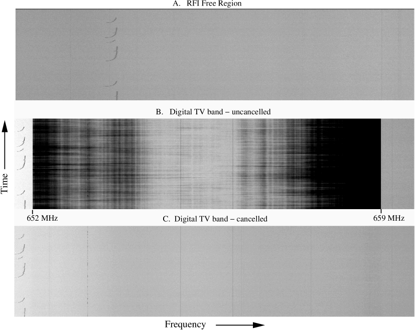
Figure 4: Dynamic spectra for A) a spectral region free of digital TV contamination, B) the spectral band containing TV channel 46, prior to cancellation, and C) the channel 46 band after cancellation.

5 Multipath delays

At first glance, multipath propagation or scattering of the interfering signal on the way from the transmitter to either the astronomical or reference antennas would appear to corrupt the interfering signal – in different ways along the paths to the different receiving systems – rendering it impossible to extract an appropriate reference signal. Fortunately, multipath is not a problem provided the paths are stable on sufficiently long time scales.

This can be easily seen by noting that the interfering signal received by an antenna $i_{r}(t)$ is the sum of different versions of the signal $i_{o}(t)$ broadcast by the transmitter at the source:

$$i_{r}(t)=\sum_{\alpha}h_{\alpha}(t)\star i_{o}(t-\tau_{\alpha})$$

Here $h_{\alpha}(t)$ is the impulse response experienced by the interfering signal along the path labeled $\alpha$, and $\star$ is the convolution operator. We have chosen to enter the relative time delays of the signal explicitly in the second term in the sum. In the frequency domain, the received spectrum $I_{r}(f)$ takes the form

$$\hskip 30.72902ptI_{r}(f) = \sum_{\alpha}G_{\alpha}(f)\>I_{o}(f)\>e^{-i2\pi\tau_{\alpha}f}$$ (7)

$$= I_{o}(f)\sum_{\alpha}G_{\alpha}(f)\>e^{-i2\pi\tau_{\alpha}f}$$

$$= I_{o}(f)\>G_{tot}(f)$$

where all the ugly details of the multipathing are contained in the single complex gain $G_{tot}(f)=\sum G_{\alpha}(f)\>e^{-i2\pi\tau_{\alpha}f}$, and the $I_{o}(f)$ stands cleanly apart. $G_{tot}(f)$ is likely to have strong frequency dependence, caused by differential phase winding from the relative delays. Clearly, application of algorithms such as Eqns 4 and 4 will require spectral resolution for the frequency channels of $\Delta f<1/\tau_{max}$, where $\tau_{max}$ is the greatest relative delay. The equivalent statement for algorithms that operate in the time domain is that the number of lags used in constructing corrective filters must be sufficiently great to capture the full range of delays.

6 Eigen Decomposition and Gain Calibration

Interferometer arrays measure correlations between the signals arriving at the array elements. Correlation matrices, such as shown in Fig. 5, can be used to summarize the covariances of the signals throughout each integration time. Since astronomers seek to detect sources that are too weak to detect in the short time of a correlator dump interval, they extract information from the measured covariances (or fringe visibilities) by searching for subtle correlations through inversion of the fourier integral of Eqn. 1. This is an effective way of reorganizing the correlation information by restricting the range of interest to only those signals that could have originated from within the field of view of their telescopes’ primary beams $p_{B}(x,y)$. Since the Earth’s rotation causes the $u$,$v$ values to change over time, the coefficients of the covariance matrix are expected to change with time; making maps is an efficient way to recover the correlations in a physically meaningful way.

There are other powerful mathematical tools for recovering information from correlation matrices, although these are geared for studying correlations over the short integration times for which the coefficients are expected to remain constant. For example, Leshem, van der Veen and Boonstra ([Leshem et al 2000], plus extensive references in [Boonstra et al 2004]) have extended the eigen decomposition methods of signal processing to applications in radio astronomy to capitalize on these tools in the area of rfi mitigation. Here, we convey some of the more intuitive conclusions to the astronomy audience.

6.1 The covariance matrices

To begin, Fig. 5 displays a full set of cross power spectra for a short observation with the Australia Telescope Compact Array – with the spectra positioned according to their positions in a correlation matrix. This data set is “srtca01” from Bell et al.’s baseband recordings ([Bell et al 2001]) taken specifically for the purpose of testing rfi mitigation algorithms. The recordings include the time sequenced sampling of the outputs from 5 antennas with two polarizations, plus two outputs from a dual polarized reference antenna aimed at the source of interference, for a total of 12 input data streams. The recorders captured 4 MHz bands with 4 bit precision. Correlation, to obtain 512 spectral channels, and integration were performed in software ([Kocz 2004]). The rfi affects the central $\sim$150 spectral channels.

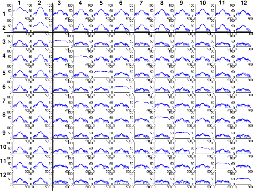
Figure 5: Examples of Power Spectra (diagonal elements) and Cross-Power Spectra (off diagonals) for a 12 signal cross correlation analysis. Each spectrum has 512 spectral channels with amplitudes in db. The upper left $2{\times}2$ grouping contains the spectra and cross power spectra for the reference channels. The lower right $10{\times}10$ group has the spectra for the 5 antennas, with 2 polarizations each, for the ATCA telescopes. The $2{\times}10$ and $10{\times}2$ groups to the lower left and upper right respectively contain the cross correlation spectra that couple the reference antennas to the ATCA signals.

The total power and cross power spectra in Fig. 5 illustrate several points: The spectra formed from the reference data streams, 1 and 2, in the upper left show that the rfi is nearly 100% linearly polarized, as it appears with equal strength in the total and cross power spectra. Further, the cross power spectra for 1–2 show that the noise in the passband outside the $\sim$150 contaminated channels integrates down to a much lower level than in these spectral ranges of the total power spectra for either 1–1 or 2–2; indeed, this is the motivation for using the cross power spectrum instead of a total power spectrum in the denominator of the correction term in Eqns. 4 and 4. Similarly, the total power spectra along the diagonal of the matrix in the lower right panels of Fig. 5 (involving inputs 3 through 12) scarcely show the presence of the rfi in several cases, but the rfi clearly appears above the noise in cross power spectra involving the same antennas.

6.2 The eigen decomposition

The eigen decomposition of a 12${\times}$12 covariance matrix solves for signals that are in common among the 12 input data streams. Since there are actually 512 covariance matrices (one for each of the 512 frequency channels), the decomposition must be performed 512 times. In matrix notation, one 12${\times}$12 covariance matrix C,

$$\textbf{C}=\left(\begin{array}[]{llll}C_{1\>1}&C_{1\>2}&...&C_{1\>12}\\ C_{2\>1}&C_{2\>2}&...&C_{2\>12}\\ C_{3\>1}&C_{2\>2}&...&C_{3\>12}\\ &...\\ C_{12\>1}&C_{12\>2}&...&C_{12\>12}\end{array}\right)$$

decomposes to the product of three 12${\times}$12 matrices: $\textbf{C}=\textbf{G}\textbf{P}\textbf{G}^{H}$, where $\textbf{G}^{H}$ is the Hermitian conjugate of G and P is a diagonal matrix containing the eigenvalues.

$$\textbf{P}=\left(\begin{array}[]{ccccc}P_{1}&0&0&...&0\\ 0&P_{2}&0&...&0\\ 0&0&P_{3}&...&0\\ &...\\ 0&0&0&...&P_{12}\end{array}\right)$$

It is convenient to think of the $P_{i}$ eigenvalues as powers. Standard methods for performing the eigen decomposition, such as singular value decomposition (SVD), produce an ordered list of eigenvalues starting with the maximum. Should the system have fewer than 12 signals present, the matrix would become singular, and some number of eigenvalues would be zero. This is not expected of a radio astronomical system, where there are not only rfi signals and celestial sources but also each input data stream brings its own noise signal.

The matrix G containing the eigenvectors

$$\textbf{G}=\left(\begin{array}[]{llll}g_{1\>1}&g_{1\>2}&...&g_{1\>12}\\ g_{2\>1}&g_{2\>2}&...&g_{2\>12}\\ g_{3\>1}&g_{2\>2}&...&g_{3\>12}\\ &...\\ g_{12\>1}&g_{12\>2}&...&g_{12\>12}\end{array}\right)$$

can be visualized as a matrix of complex voltage gains $g_{ij}$, giving the coupling of each signal (whose voltage is $P_{i}^{1/2}$) to the covariances. Thus, the amount of $P_{i}$ coupled to $C_{jk}$ is $g_{ji}g_{ki}^{*}P_{i}$. The top row of G specifies the coupling of the 12 $P_{i}$ to the number 1 input, which is the first reference antenna in the example here.

Figure 6 shows the eigenvalue spectra obtained from 512 eigen decompositions that were performed one spectral channel at a time for the data in Fig. 5. The calculation has succeeded in separating the rfi and concentrating its power in the first eigenvalue $P_{1}(f)$. The other $P_{i}(f)$ for $i>1$ appear to represent normal passband power levels expected from receiving systems dominated by internal noise. The one exception is a narrow rfi spike in $P_{2}(f)$ around channel 290 that had not been apparent in the spectra in Fig. 5.

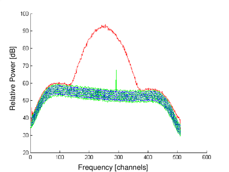
Figure 6: Eigenvalue Spectra for $P_{i}(f)$ for $i$=1,12. Except for $P_{1}(f)$, the spectra are very closely spaced, and the 11 parallel “passbands” are drawn in alternating light and dark colors.

6.3 Special case: Array calibration

An analogy can be made to a common procedure in the amplitude and phase calibration of synthesis arrays. Typically, an observation is performed on a bright, unresolved radio continuum source, whose flux density $S_{\nu}$ is high enough that the source’s power in the receiving system will dominate over all other powers after a short integration time. In the notation above, this condition means that there is one dominant eigenvalue $P_{1}=S_{\nu}$. Under this condition, the P matrix degenerates to 1$\times$1, and the eigenvector matrix G becomes an 12$\times$1 dimensional vector of complex gains. In fact, the standard methods of array calibration solve for the “antenna based complex gain factors” (for amplitude and phase). These gains are a subset of the full eigenvector array, but they enable the reconstruction of the covariance matrix for the case with a single powerful source.

$$\textbf{C}=\left[\begin{array}[]{l}g_{1}\\ g_{2}\\ g_{3}\\ ...\\ g_{12}\end{array}\right]\left[S_{\nu}\right]\left[g_{1}^{*}\>g_{2}^{*}\>g_{3}^{*}\>...\>g_{12}^{*}\right]$$

6.4 Nulling

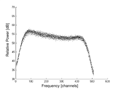
Figure 7: Total power spectra for astronomy channels (3-12) after partial nulling the dominant eigenvalue.

Having identified the strength and spectral behavior of the rfi through its dominance in the eigen decomposition of Fig. 6, one is tempted to null the rfi by replacing $P_{1}$ by zero. However, this would be slightly too severe a partitioning of the eigenvalue matrix, since this would also remove the system noise contribution and perhaps distort a weak celestial signal contributing noise power to the system. In these illustrations reported here, we replace $P_{1}(f)$ by the average of the other $P_{i}(f)$ ($i$=2,12), and then reconstruct the covariances $\textbf{C}(f)$ from G and the modified P matrix. This produces the total power spectra for the ten telescope data streams as shown in Fig. 7 and the two reference antenna data streams in Fig. 8.

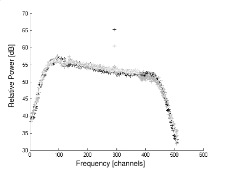
Figure 8: Total power spectra for reference channels (1-2) after partial nulling the dominant eigenvalue.

The partial nulling of the dominant eigen value has been effective in recovering total power spectra for the telescope inputs (3–12) in which no remnant of the rfi is visible. The partial nulling has also removed the rfi from the reference inputs (1 and 2), allowing the second, narrow interferer from $P_{2}$ to be seen in the spectra for both. Apparently, this narrow interferer was only picked up by the reference antennas and not by the ATCA telscopes themselves.

The process adopted here to partially null the eigenvalue and then recompute an edited covariance matrix has the identical effect to the procedure in which the unwanted portion of the eigenvalue P matrix is “projected” back into the covariance matrix and then subtracted (e.g. [Leshem et al 2000]).

6.5 Directional information from the eigen decomposition

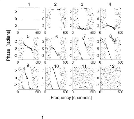
Figure 9: Eigenvector phases for the dominant eigenvalue for all 12 data channels.

In the worked example for 12 input data streams, the eigen decomposition has identified two interfering sources based on the mathematical interpretation of the convariance matrix, and it has also enabled the nulling of the rfi power. This is accomplished without knowledge of location of the interferer, aside from having aimed the reference antennas; in fact, basing the analysis on the 10 inputs from the ATCA dishes alone (and ignoring the reference antenna inputs) leads to a similar result, albeit with a lower interference-to-noise ratio in the eigenvalue spectra ([Kocz 2004]).

There is directional information contained in the phases of the complex eigenvector coefficients. To illustrate this, Fig. 9 plots the phase spectra for the $g_{1j}$ coefficients that couple $P_{1}$ (the dominant eigenvalue containing the strong rfi power) to each of the array antennas. Outside the central channels, the phases become random, implying that there is no strong broadband signal in these spectral ranges to influence these spectral channels. In the center of the band where the rfi is strong, the phases show the characteristic drift with frequency that is expected for interferometer baselines of increasing length (and therefore increasing delay) as indicated in Eqn. 7. The baseline length to the ATCA telescope number 6 was much longer that the other baselines between the telescopes during this experiment, so the phases for data streams 11 and 12 that were produced by telescope 6 wind very rapidly as a function of frequency across the band and therefore are not detected by eye in Fig. 9. Radio astronomers might expect to decode this phase information to infer directional information about the origin of rfi signals – a process that would be straight forward if the positions of the elements of the array were well known and the element gains were isotropic. In practice, the use of directional information is hampered by the unknown and variable gains of the sidelobes through which the RFI enters the antenna ([Leshem et al 2000]).

6.6 Subtleties and cautions

The eigen decomposition approach shows promise for some applications in rfi mitigation. There are some subtleties to its application that are covered in greater depth in the series of papers by Leshem et al (e.g., [Leshem et al 2000]). (1) Among these is the need to prewhiten the noise among the input channels in order for the algorithm to perform well; this is a step that would require some care in calibration of an array. (2) Further, there is the question touched upon in section 6.4 where setting the dominant eigenvalue to zero was attempted in order to null the rfi; there is some subtlety in how to choose the right amount to remove and how much to leave behind, given that the signals from celestial sources are likely to appear weakly in the eigenvalues. (3) Astronomical covariance matrices generally carry signals from more sources than the dimensionality of the matrix. While rfi might produce the strongest signals, causing them to stand out in the eigen decomposition, there is also noise signal associated with each of the telescope inputs, as well as with the signals from numerous weak celestial radio sources. Once the number of signals exceeds the number of inputs to the correlator, a complete recovery of the separate signals is no longer possible; in effect, the number of unknowns exceeds the number equations available for solution. Even the eigen values are then mixtures of signals, and the process of nulling runs the risk of damaging the astronomical signals.

7 Summary

This paper gave an overview of a couple of methods for rfi cancellation that show promise for application in radio astronomy observations. There remains considerable challenge to achieving the dynamic range in rfi cancellation likely to be required.