The mass of the black hole in 3C 273

In this paper we apply the reverberation method to determine the mass of the black hole in 3C 273 from the Ly$\alpha$ and Civ emission lines using archival IUE observations. Following the standard assumptions of the method, we find a maximum-likelihood estimate of the mass of $6.59\,10^{9}$ M_⊙, with a $1\sigma$ confidence interval $5.69-8.27\,10^{9}$ M_⊙. This estimate is more than one order of magnitude larger than that obtained in a previous study using Balmer lines. We reanalyze the optical data and show that the method applied to the H$\alpha$, H$\beta$, and H$\gamma$ Balmer lines produce mass estimates lower by a factor 2.5, but already much larger than the previous estimate derived from the same lines. The finding of such a high mass in a face-on object is a strong indication that the gas motion is not confined to the accretion disk. The new mass estimate makes 3C 273 accreting with an accretion rate about six times lower than the Eddington rate. We discuss the implications of our result for the broad-line-region size and black-hole mass vs luminosity relationships for the set of objects for which reverberation black-hole masses have been obtained. We find that, while objects with super-Eddington luminosities might theoretically be possible, their existence is not necessarily implied by this sample.

1 Introduction

As soon as the variability of the broad emission lines in Seyfert 1 galaxies and QSOs had been discovered, its potential for the investigation of the structure of these objects became evident. Gaskell & Sparke (1986) were the first to propose using cross-correlation methods between the continuum and line light curves to measure the size of the broad-line region (BLR). The subsequent building of long and dense spectro-photometric light curves of broad-line active galactic nuclei (BL-AGN), in particular thanks to the IUE satellite and to the AGN Watch consortium (Alloin et al. 1994), made the reliable measurement of the BLR size in a significant number of objects possible. The so-called reverberation method was later developed to allow a determination of the mass of the central black hole (Peterson & Wandel 1999; Wandel et al. 1999), under the assumption that the gas dynamics is dominated by gravity and using the fact that its velocity dispersion can be deduced from the width of the line. The connection between black-hole mass and line widths in BL-AGN has allowed the development of methods to determine the black-hole masses in high-redshift QSOs (Vestergaard 2002; McLure & Jarvis 2002), and thus opened the door to cosmological studies of black holes. These methods require, however, a good understanding of the relationship between luminosity and BLR size, which must be investigated through the use of the reverberation method.

Krolik (2001) warned that some assumptions made in the context of the reverberation method are not sufficiently validated. A key assumption is that the gas dynamics is dominated by the gravitational pull from the central black hole. While Peterson & Wandel (1999) showed that the $v\propto r^{-1/2}$ relationship expected in such case is satisfied in NGC 5548 for different lines, other competing models can also explain this dependence. The best support for the assumptions behind the reverberation method is the agreement between the reverberation masses and those obtained using stellar-velocity dispersion (Gebhardt et al. 2000). Merritt & Ferrarese (2001) also concluded that the reverberation-mass estimates are not more strongly biased than stellar velocity-dispersion ones. The existence of hidden assumptions nevertheless makes Krolik (2001) conclude that, even if valid, the method is subject to systematic uncertainties as large as a factor 3 or more.

In a previous paper (Paltani & Türler 2003, hereafter Paper I), we studied in detail the response of the Ly$\alpha$ and Civ emission lines in 3C 273. In this paper, we extend our study by applying the reverberation method to determine the mass of the central black hole in this object. We make the assumption that the reverberation method is valid and apply the methodology presented in Wandel et al. (1999) to derive the black-hole mass using the strongest broad ultraviolet lines: Ly$\alpha$ and Civ. We differ with previous works on the treatment of statistical errors and propose here a full error propagation, in order to obtain meaningful confidence intervals on our results. We also compare our results with those in the optical domain from Kaspi et al. (2000). We finally assess the consequence of our results on two important relationships in BL-AGN: the broad-line-region size vs luminosity and black-hole mass vs luminosity relationships.

2 Data

This paper makes use of data from the 3C 273 database hosted by the Geneva Observatory and presented in Türler et al. (1999). We use the same data set as in Paper I, namely the IUE short wavelength (SWP) spectra processed with the IUE Newly Extracted Spectra (INES) software (Rodríguez-Pascual et al. 1999). Details of data preparation can be found in Paper I, but we summarize below the main properties of the sample for completeness.

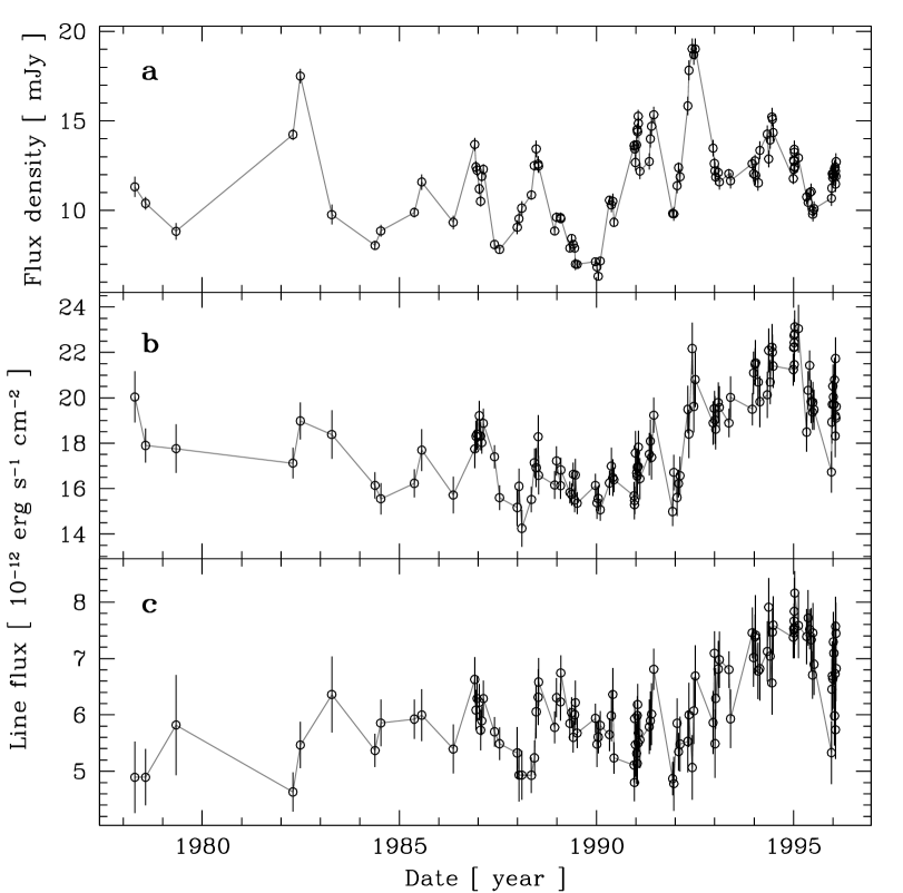
Our light curves each consist of 119 observations covering 18 years, including a ten-year period with semi-weekly observations during two annual observation periods of 3 months, separated by two months. From the original 256 SWP observations, over- and underexposed observations were discarded, and observations taken within 12 hours were averaged. The Ly$\alpha$ $\lambda$1216 and Civ $\lambda$1549 fluxes were integrated above a continuum defined by a straight line fitted to the points in two 50 Å continuum bands on each side of the lines. We integrate the total Ly$\alpha$ and Civ line fluxes for projected rest-frame velocities up to $\pm 20\,000$ km s^-1 and $\pm 10\,000$ km s^-1 respectively. Uncertainties on the line fluxes take into account the uncertainty in the underlying continuum and the number of independent bins. The Ly$\alpha$ emission line is contaminated by Nv $\lambda$1240 emission. In the following, “Ly$\alpha+$Nv” will be used to designate the full line profile around Ly$\alpha$, which includes the Nv contamination, and “Ly$\alpha-$Nv” to designate the line profile around Ly$\alpha$ where the range 3500–10 000 km s^-1 has been linearly interpolated to get rid of the Nv contamination.

Figure 1 shows the three main light curves used in this study: the 1250–1300 Å continuum, the integrated Ly$\alpha+$Nv emission line, and the integrated Civ emission line. All light curves used in this paper are listed in Table 1 of Paper I, which is available electronically. They can also be downloaded from the 3C 273 database.

Figure 1: (a) Ultraviolet continuum light curve averaged in the 1250–1300 Å band. (b) Ly$\alpha+$Nv emission line light curve integrated for velocities up to 20 000 km s^-1. (c) Civ emission line light curve integrated for velocities up to 10 000 km s^-1.

3 Black-hole mass

We estimate the mass of the black hole in 3C 273 using the reverberation method introduced by Peterson & Wandel (1999). The line-emitting gas is assumed to be in virial equilibrium around a mass dominated by the black hole, so that the gas distance to the central object and its velocity dispersion are both related to the mass through the virial theorem. The velocity dispersion can be estimated from the line width, and the gas distance from the delay between the continuum and line light curves, making possible a determination of the mass. In principle, a single line is sufficient. The consistency of mass estimates from different lines is, however, a stringent test of the validity of the method.

In Paper I, we showed that the Ly$\alpha$ and Civ emission lines show two distinct components. We interpreted the second component as evidence of gas entrainment in the course of an interaction with the jet. In principle, the presence of a non-virial velocity field makes the above method inapplicable; however, we showed that this component mostly affects the blue wings of the lines, making the red sides (hereafter, the “red profiles”) suitable for a mass determination. We nevertheless perform the analysis both on the full lines and on the red profiles for comparison. We also perform the analysis separately on Ly$\alpha+$Nv and Ly$\alpha-$Nv to evaluate the effect of contamination by Nv.

In this work, we shall make sure to correctly propagate all uncertainties in our data into the determination of the mass. As the error distributions of the lag and velocity dispersion are not at all Gaussian, they cannot be combined analytically to determine the confidence intervals on the black-hole mass. We thus construct the full black-hole mass error distribution using those of the lag and of the velocity dispersion.

3.1 Distance of the line-emitting gas

The distance of the line-emitting gas to the source can be estimated using the delay between the line and ionizing-continuum (or its closest approximation) light curves. Delays can be readily obtained using a cross-correlation analysis. However, as the gas fills a vast range of distances, there is no unique way to derive a delay from a cross-correlation. Koratkar & Gaskell (1991b) have argued that the centroid of the cross-correlation function gives the emissivity-weighted average radius of the emission region.

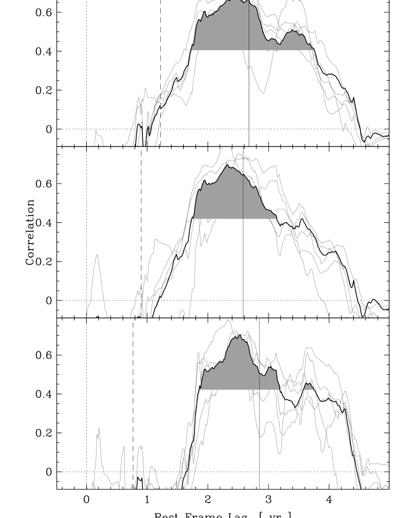
We follow here the method proposed by Peterson et al. (1998). We calculate the cross-correlations between the continuum (in the 1250–1300 Å band) and the Ly$\alpha+$Nv, Ly$\alpha-$Nv, and Civ light curves. We use the Interpolated Cross-Correlation Function (ICCF) of Gaskell & Peterson (1987) with the improvements introduced by White & Peterson (1994). The delay is estimated by calculating the average lag weighted by the correlation coefficient for all those parts of the cross-correlation which exceed a given threshold $\vartheta$ expressed as a fraction of the maximum correlation. This is illustrated in Fig. 2 for the actual Ly$\alpha+$Nv and Civ correlations.

Figure 2: Cross-correlation between the UV continuum and the red-profile Ly$\alpha+$Nv (top) and Civ (bottom) light curves. In both panels, the shaded area represents the parts of the correlation above the threshold set at 60% of its maximum (i.e. $\vartheta=0.6$). Only these areas are used in the estimation. The average lag is indicated by a vertical line. Five realizations of the FR/RSS method are also shown in each panel for illustration.

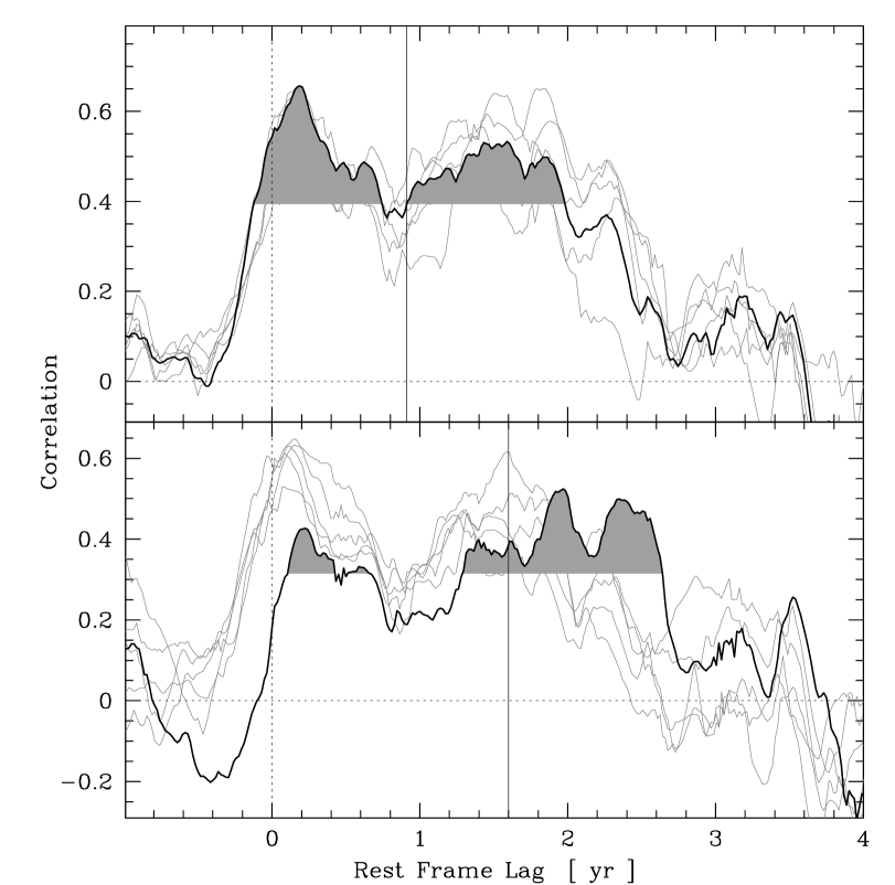
The lag distribution is estimated using the flux-randomization/random-subset-selection (FR/RSS) method of Peterson et al. (1998): Both line and continuum fluxes are first randomized according to their uncertainties, and 119 dates are drawn at random (with possible repetitions) from the original dates. The two light curves are then cross-correlated, and a new lag estimate is produced. The lag error distribution is then constructed from the distribution of lag estimates. Examples of FR/RSS realizations are shown in Fig. 2.

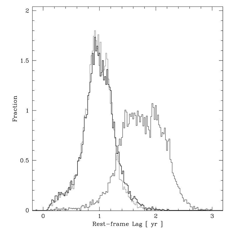
Because one wants to take into account as much gas as possible, the threshold should be set as low as possible. However, if taken too low, non-significant parts of the correlation function are included in the lag estimate. Considering the flat-top correlation functions we observe here, high thresholds seem inappropriate, as they make the result quite dependent on small details of the correlation functions. We adopt here a threshold of 0.6, but we checked that the choice of the threshold has a moderate impact of about 30% on the average delay throughout the range $0.3\leq\vartheta\leq 1$. The error distributions, however, become very large and are no longer unimodal as soon as $\vartheta>0.8$, which shows that the lags start being dominated by non-significant details of the correlation function. The average lags and the confidence intervals are given in Table 1. All lags are expressed in the object’s rest frame. In both Ly$\alpha$ and Civ lines, the lags of the full profiles are systematically larger than their corresponding lags in the red profiles, consistent with the results of Paper I. The individual differences are not statistically significant however. The effect of Nv is completely negligible. Error distributions of the lags for the red profiles are shown on Fig. 3.

Table 1: Average rest-frame lags in years of the Ly$\alpha$ and Civ emission lines. The numbers in brackets give the $\pm 1\sigma$, $\pm 2\sigma$, and $\pm 3\sigma$ confidence intervals.

Line	Full profile	Red profile
Ly$\alpha+$Nv	$1.19\leavevmode\nobreak\ \left\{{}_{-0.21}^{+0.21}\right.\left\{{}_{-0.46}^{+0.50}\right.\left\{{}_{-0.86}^{+0.79}\right.$	$0.97\leavevmode\nobreak\ \left\{{}_{-0.24}^{+0.25}\right.\left\{{}_{-0.63}^{+0.54}\right.\left\{{}_{-0.85}^{+0.92}\right.$
Ly$\alpha-$Nv	$1.21\leavevmode\nobreak\ \left\{{}_{-0.20}^{+0.20}\right.\left\{{}_{-0.44}^{+0.49}\right.\left\{{}_{-0.82}^{+0.79}\right.$	$0.98\leavevmode\nobreak\ \left\{{}_{-0.26}^{+0.27}\right.\left\{{}_{-0.68}^{+0.60}\right.\left\{{}_{-0.86}^{+1.00}\right.$
Civ	$1.89\leavevmode\nobreak\ \left\{{}_{-0.29}^{+0.28}\right.\left\{{}_{-0.53}^{+0.55}\right.\left\{{}_{-0.89}^{+0.80}\right.$	$1.75\leavevmode\nobreak\ \left\{{}_{-0.37}^{+0.39}\right.\left\{{}_{-0.80}^{+0.69}\right.\left\{{}_{-1.49}^{+1.08}\right.$

Figure 3: Lag error distribution for the red profiles of the Ly$\alpha-$Nv (black), Ly$\alpha+$Nv (light grey), and Civ (dark grey) emission lines

3.2 Line velocity dispersion

The velocity dispersion of the emitting gas can be estimated using the shape of the line. In the context of mass determination, line velocity dispersion is generally determined from the full width at half maximum (FWHM) of the rms profile (Wandel et al. 1999). This profile is then used to avoid contamination from a possible stable narrow-line component. The relationship between FWHM and gas velocity dispersion relies, however, on assumptions about the line shape that are difficult to assess. In addition, the measurement of the FWHM is very sensitive to details of the profile. Fromerth & Melia (2000) propose to calculate the squared velocity dispersion directly from the second moment of the line profile:

$$<\!v^{2}\!>=3\left(\frac{\int P(v)v^{2}{\mathrm{d}}v}{\int P(v){\mathrm{d}}v}-\left(\frac{\int P(v)v{\mathrm{d}}v}{\int P(v){\mathrm{d}}v}\right)^{2}\right),$$ (1)

where $P(v)$ is the amplitude of the rms profile at rest-frame velocity $v$. The only assumption behind this method is the isotropy of the emission, which is the origin of the factor 3 in the above equation.

Figure 4 shows the two rms profiles of the Ly$\alpha+$Nv and Civ emission lines.

Figure 4: Continuum-subtracted rms profiles of the Ly$\alpha+$Nv (top) and Civ (bottom) emission lines. The grey area marks the region of the Ly$\alpha$ profile contaminated by Nv emission line.

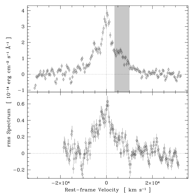
The rms profiles are rather complex, presenting a narrow core, broad wings and secondary peaks, and are not easily represented by a simple analytic form. This is the kind of situation to which the method of Fromerth & Melia (2000) is particularly adapted; in the following, we adopt Eq. (1) to calculate the velocity dispersion.

It is not clear how the error distribution of the velocity dispersion can be calculated. Kaspi et al. (2000) use the FWHM dispersion measured in individual spectra as an estimate of the uncertainty in the FWHM of the rms profile, but there is no obvious reason why it would give the correct result. Here we follow a different approach: The uncertainty in any point of the rms profile can be estimated using the standard estimator of error on the rms: $\sigma_{\mathrm{rms}}(\lambda)=\mathrm{rms}(\lambda)/\sqrt{2(N-1)}$, where $N$ is the number of spectra. However, the rms in different wavelength bins will be strongly correlated with each other, because they have been obtained using the same spectra. Thus we scale the uncertainties on the rms profile by requiring that the average uncertainty of the rms profile in the continuum regions is equal to the standard deviation of the rms estimates. We can then estimate the velocity-dispersion distribution by randomizing the rms profiles a large number of times according to the uncertainties in each bin before continuum subtraction (so that the error on the continuum determination is included in our determination), and by measuring the velocity dispersion using Eq. (1) for each of them.

Table 2 gives the velocity dispersions of the Ly$\alpha$ and Civ emission lines obtained with the 2nd-moment method. Figure 5 compares the velocity-dispersion error distribution for the red profiles of Ly$\alpha-$Nv and Civ. We removed a spectral bin close to the center of the Civ line with a linear interpolation, because it was strongly affected by a reseau mark.

Table 2: Average velocity dispersions in km s^-1 of the Ly$\alpha$ and Civ emission lines. The numbers in brackets give the $\pm 1\sigma$, $\pm 2\sigma$, and $\pm 3\sigma$ confidence intervals.

Line	Full profile	Red profile
Ly$\alpha+$Nv	$10\,044\leavevmode\nobreak\ \left\{{}_{-423}^{+423}\right.\left\{{}_{-892}^{+812}\right.\left\{{}_{-1341}^{+1119}\right.$	${\phantom{1}}9\,941\leavevmode\nobreak\ \left\{{}_{-539}^{+532}\right.\left\{{}_{-1133}^{+{\phantom{1}}996}\right.\left\{{}_{-1909}^{+1431}\right.$
Ly$\alpha-$Nv	${\phantom{1}}9\,955\leavevmode\nobreak\ \left\{{}_{-178}^{+179}\right.\left\{{}_{-366}^{+347}\right.\left\{{}_{-{\phantom{1}}575}^{+{\phantom{1}}512}\right.$	${\phantom{1}}9\,707\leavevmode\nobreak\ \left\{{}_{-240}^{+240}\right.\left\{{}_{-{\phantom{1}}491}^{+{\phantom{1}}461}\right.\left\{{}_{-{\phantom{1}}738}^{+{\phantom{1}}674}\right.$
Civ	${\phantom{1}}8\,049\leavevmode\nobreak\ \left\{{}_{-346}^{+352}\right.\left\{{}_{-738}^{+667}\right.\left\{{}_{-1129}^{+1003}\right.$	${\phantom{1}}7\,795\leavevmode\nobreak\ \left\{{}_{-436}^{+442}\right.\left\{{}_{-{\phantom{1}}947}^{+{\phantom{1}}828}\right.\left\{{}_{-1557}^{+1137}\right.$

Figure 5: Velocity-dispersion error distributions of the red profiles (continuous lines) and full profiles (dashed lines) of the Ly$\alpha-$Nv (black), Ly$\alpha+$Nv (light grey), and Civ (dark grey) rms profiles.

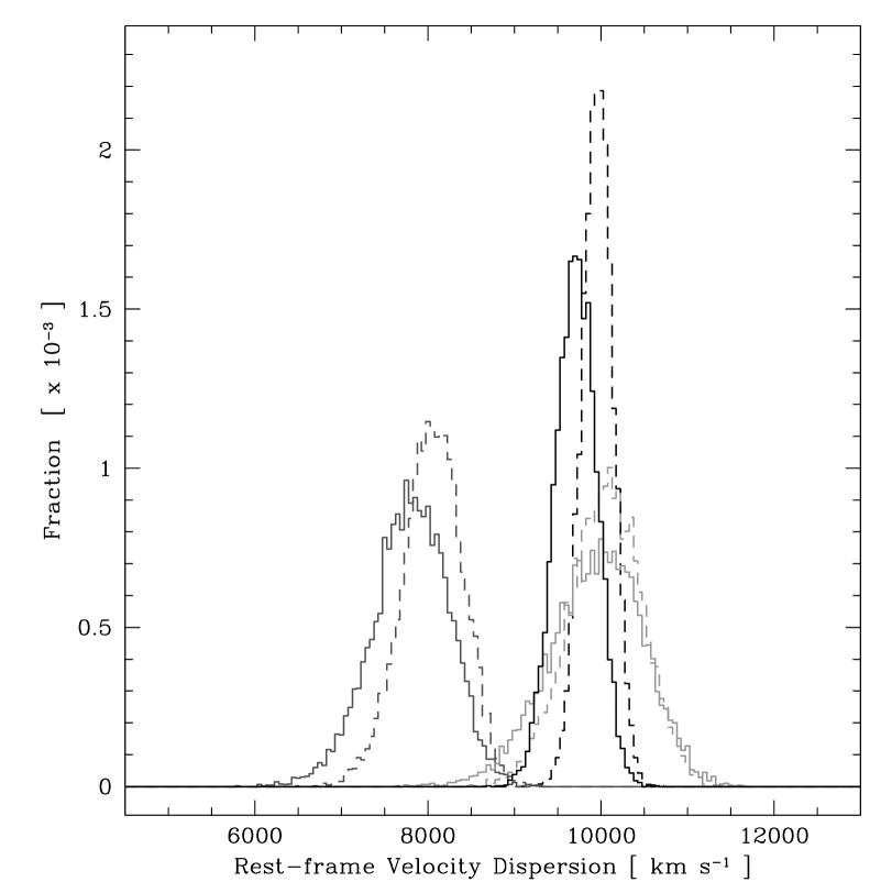
The effect of removing Nv is sufficiently small so that we can exclude a strong residual Nv contamination in Ly$\alpha-$Nv. The effect of asymmetry on the measurement of the velocity dispersion is approximately 3% in both Ly$\alpha-$Nv and Civ. This consistency shows that the line is dominated by a symmetric velocity component, assumed to be due to Keplerian motion, but the broadening of the full profile with respect to the red profile, although not significant, is systematic.

3.3 Mass determination

The velocity dispersion and delay can be combined to obtain the black hole mass from the virial equation:

$$M_{\mathrm{BH}}=71.31\leavevmode\nobreak\ \tau<\!v^{2}\!>\mathrm{M}_{\odot}$$ (2)

where $\tau$ is the lag expressed in units of years and $<\!\!v^{2}\!\!>$ the squared velocity dispersion expressed in units of km s^-1. This formula is identical to Eq. (6) of Wandel et al. (1999), except that the velocity dispersion is used instead of the FWHM. As in Peterson & Wandel (1999), the factor between the kinetic and potential energies in the virial theorem is set more or less arbitrarily to $-1$. Error distributions of the masses are constructed using a Monte-Carlo approach. We draw a large number of pairs of random values from the error distributions of the lags and velocity dispersions, and combine them using Eq. (2) to obtain the error distributions of the masses. The results are given in Table 3.

Table 3: Average black-hole masses of 3C 273 in units of $10^{9}\,$M_⊙. The numbers in brackets give the $\pm 1\sigma$, $\pm 2\sigma$, and $\pm 3\sigma$ confidence intervals. $\hat{M}$ is the maximum-likelihood mass obtained from the combination of Ly$\alpha-$Nv and Civ emission lines.

Line	Full profile	Red profile
Ly$\alpha+$Nv	$8.56\leavevmode\nobreak\ \left\{{}_{-1.68}^{+1.72}\right.\left\{{}_{-3.50}^{+4.01}\right.\left\{{}_{-6.04}^{+6.40}\right.$	$6.83\leavevmode\nobreak\ \left\{{}_{-1.88}^{+1.91}\right.\left\{{}_{-4.52}^{+4.25}\right.\left\{{}_{-6.02}^{+7.10}\right.$
Ly$\alpha-$Nv	$8.56\leavevmode\nobreak\ \left\{{}_{-1.40}^{+1.47}\right.\left\{{}_{-3.19}^{+3.51}\right.\left\{{}_{-5.74}^{+5.91}\right.$	$6.59\leavevmode\nobreak\ \left\{{}_{-1.77}^{+1.83}\right.\left\{{}_{-4.55}^{+4.07}\right.\left\{{}_{-5.79}^{+6.67}\right.$
Civ	$8.75\leavevmode\nobreak\ \left\{{}_{-1.53}^{+1.53}\right.\left\{{}_{-2.79}^{+3.15}\right.\left\{{}_{-4.41}^{+4.90}\right.$	$7.62\leavevmode\nobreak\ \left\{{}_{-1.80}^{+1.90}\right.\left\{{}_{-3.64}^{+3.77}\right.\left\{{}_{-6.50}^{+6.20}\right.$
$\hat{M}$	$8.20\leavevmode\nobreak\ \left\{{}_{-1.14}^{+1.02}\right.\left\{{}_{-2.25}^{+2.31}\right.\left\{{}_{-3.16}^{+3.82}\right.$	$6.59\leavevmode\nobreak\ \left\{{}_{-0.90}^{+1.68}\right.\left\{{}_{-1.87}^{+3.04}\right.\left\{{}_{-3.15}^{+4.62}\right.$

Figure 6: Top panel: Black-hole mass distributions for the red profiles of the Ly$\alpha-$Nv (black), Ly$\alpha+$Nv (dashed line), and Civ (grey) emission lines. Bottom panel: Likelihood function of the mass. The horizontal grey lines show, from top to bottom, the $\pm 1\sigma$, $\pm 2\sigma$, and $\pm 3\sigma$ levels. The vertical lines show the $\hat{M}_{\pm 1}$, $\hat{M}_{\pm 2}$, and $\hat{M}_{\pm 3}$ intervals.

As expected from Paper I, the average masses obtained with the red profiles of the lines are systematically smaller than those obtained with the full profiles. The full-profile values fall however within, or close to, the $\pm 1\sigma$ red-profile confidence interval. The difference between Ly$\alpha+$Nv and Ly$\alpha-$Nv is less than 5% for the red profiles. The minimum mass at the $3\sigma$ level is about $0.8\,10^{9}$ M_⊙.

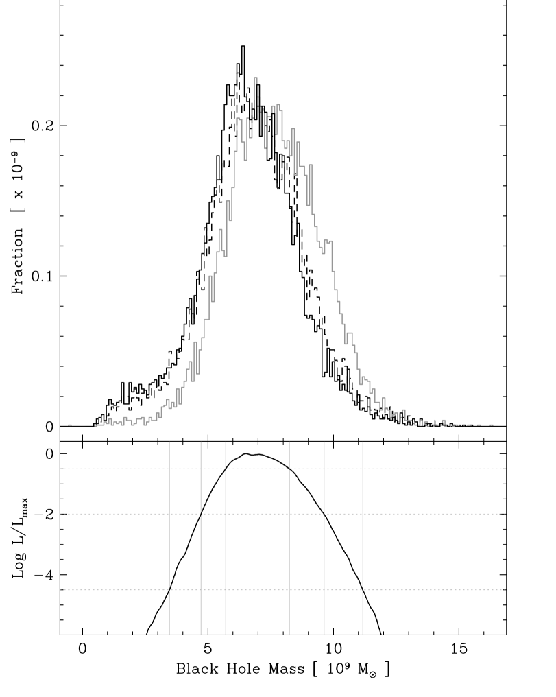
The black-hole mass distributions for the red profiles of the Ly$\alpha+$Nv, Ly$\alpha-$Nv, and Civ emission lines are shown in Fig. 6. All three distributions overlap very significantly. Confronted with several estimates of the same values, we can combine them using a $\chi^{2}$ test only if the error on the estimates have Gaussian distributions. As this is not the case here, we use a maximum-likelihood estimator (MLE), where mass is the unknown parameter that we try to recover. In the simple case of $N$ independent measurements of the same value that we consider here, the (natural) logarithm of the likelihood function is a function of the mass $M$ given by:

$$\log L(M)=\sum_{i=1}^{N}\log P_{i}(M),$$ (3)

where $P_{i}(M)$ is the probability distribution of $M$ in measurement $i$ and is approximated by our black-hole mass distributions. The MLE $\hat{M}$ is then the value of the mass that maximizes $L(M)$:

$$\frac{{\mathrm{d}}\log L(\hat{M})}{{\mathrm{d}}M}=0.$$ (4)

The $\{\hat{M}_{-n},\hat{M}_{+n}\}$ $n$-sigma confidence interval can be determined using:

$$\log L(\hat{M}_{\pm n})=\log L(\hat{M})-\frac{n^{2}}{2}.$$ (5)

Applying this method to measurements of the black hole mass for the red profiles of the Ly$\alpha-$Nv and Civ emission lines, we obtain a maximum-likelihood mass of $6.59\,10^{9}$ M_⊙. The $1\sigma$, $2\sigma$, and $3\sigma$ confidence intervals are $5.69-8.27\,10^{9}$ M_⊙, $4.72-9.63\,10^{9}$ M_⊙, and $3.44-11.21\,10^{9}$ M_⊙ respectively. The difference in the MLEs for the full and red profiles is about 1.5$\sigma$.

4 Mass derived from Balmer lines

Kaspi et al. (2000) (hereafter K00) performed a series of spectro-photometric observations in the 4500–8000 Å domain on a set of 28 QSOs, among which is 3C 273. From the Balmer lines, they obtained a mass of $0.235^{+0.037}_{-0.033}\,10^{9}$ M_⊙ from the rms profiles, and $0.550^{+0.089}_{-0.079}\,10^{9}$ M_⊙ from the average line profiles. These values are apparently the average of the masses obtained using H$\alpha$ and H$\beta$. Individual estimates of the mass for different lines and different line-width determination methods vary by a factor 5 from $0.115$ to $0.56\,10^{9}$ M_⊙, i.e. a much larger range than the $\sim\!15$% uncertainties they claim. This indicates a serious problem in their mass determination for this object. These masses are in complete disagreement with our result using Ly$\alpha$ and Civ, as they are between 12 and 60 times smaller than our maximum-likelihood determination, and at least $6$ times smaller than $\hat{M}_{-3}$.

It must first be noted that K00 determined the line lag with respect to continuum using the optical continuum around 5000 Å. Paltani et al. (1998) showed that the optical continuum properties of 3C 273 differ considerably from those of the ultraviolet continuum. They concluded that the optical emission of 3C 273 is strongly contaminated, and perhaps even dominated, by non-thermal radiation, possibly related to the jet of 3C 273, and varying on much longer time scales than the UV continuum. The optical continuum therefore appears unsuitable for studying the lag between the ionizing continuum and the lines. Using the (full-line) H$\alpha$, H$\beta$ and H$\gamma$ light curves from K00, we redetermine the lags with the same ultraviolet continuum light curve used to determine the lags with Ly$\alpha$ and Civ. In addition to using a continuum much closer to the ionizing continuum, the lag determination is improved by mutiplying by three the number of observations over a twice as long period of time. Fig. 7 shows the correlation between the UV continuum and the three Balmer lines H$\alpha$, H$\beta$, and H$\gamma$. Table 4 compares our lags with those from K00, ours being between 2 and 4 times larger. Furthermore, our estimates are in excellent agreement with each other, while in K00 the H$\alpha$ lag is 60% larger than that of H$\gamma$.

Figure 7: Cross-correlation between the UV continuum and the H$\alpha$ (top), H$\beta$ (center), and H$\gamma$ (bottom) light curves. In all three panels, the shaded area represents the parts of the correlation above the threshold set at 60% of its maximum (i.e., $\vartheta=0.6$). Only these areas are used in the weighted average of the lag (indicated by a vertical line). The dashed vertical lines indicate the lags from K00. Five realizations of the FR/RSS method are also shown in each panel for illustration.

Table 4: Average rest-frame lags in years of the H$\alpha$, H$\beta$, and H$\gamma$ emission lines found in this study compared to the values of K00. The numbers in brackets give the $\pm 1\sigma$, $\pm 2\sigma$, and $\pm 3\sigma$ confidence intervals. Only the $\pm 1\sigma$ confidence intervals are available from K00.

Line	UV-continuum lag	Optical-continuum lag
	(This work)	(K00)
H$\alpha$	$2.68\leavevmode\nobreak\ \left\{{}_{-0.15}^{+0.14}\right.\left\{{}_{-0.36}^{+0.33}\right.\left\{{}_{-0.56}^{+0.58}\right.$	$1.22\leavevmode\nobreak\ \left\{{}_{-0.16}^{+0.15}\right.$
H$\beta$	$2.58\leavevmode\nobreak\ \left\{{}_{-0.19}^{+0.19}\right.\left\{{}_{-0.33}^{+0.41}\right.\left\{{}_{-1.20}^{+0.71}\right.$	$0.90\leavevmode\nobreak\ \left\{{}_{-0.22}^{+0.28}\right.$
H$\gamma$	$2.85\leavevmode\nobreak\ \left\{{}_{-0.32}^{+0.32}\right.\left\{{}_{-0.69}^{+0.71}\right.\left\{{}_{-2.63}^{+1.00}\right.$	$0.77\leavevmode\nobreak\ \left\{{}_{-0.25}^{+0.14}\right.$

The velocity dispersion measurements in K00 are also problematic for 3C 273. The rms widths of the Balmer lines in 3C 273 reported by K00 are completely incompatible with each other, differing by a factor 2.5, while the quoted uncertainties on the widths are only about 2–6%. Such disagreements are absent in most objects of their sample. As we do not have access to the spectra used in K00, we use two spectro-photometric observations performed with the STIS instrument (O44301010 for H$\gamma$ and O44301020 for H$\beta$ and H$\alpha$) on the Hubble Space Telescope. Without variability information, we have to apply the second-moment method to the average profile (calculated with a single profile) instead of the rms profile. The continuum and line regions were defined exactly as in K00. In theory, the line width can be reduced by the presence of narrow-line Balmer emission, but K00 showed that the effect over their whole sample is small. Because of strong [O iii] 4959Å and 5007Å contamination in the red profile of H$\beta$, we used only the blue profile of this line. Some contaminating emission lines are present in the H$\alpha$ and H$\gamma$ profiles, but we checked that the blue and red profiles give results in good agreement, showing that the contamination is probably small. The errors on these values were arbitrarily set to 10%, because, if calculated as in the case of the UV lines, the formal errors would be unrealistically low. Table 5 compares our velocity dispersions with those in K00. Except for H$\alpha$, which is 80% larger, the widths obtained here are comparable to those in K00 using the mean profile. The rms velocity-dispersion measurements of K00 for H$\beta$ and H$\gamma$ are about 15–25% smaller, and the discrepancy reaches a factor 4 for H$\alpha$. Considering that the K00 values for the different Balmer lines using the mean profile differ by 25% and those using the rms profile by a factor 2.5, it seems to us that there could be a problem in their rms profile determination, which could easily result from one or two bad spectra.

Table 5: Average velocity dispersions in km s^-1 of the three Balmer lines found in this study compared to the values of K00 with the rms and average (mean) profiles. The numbers in brackets give the $\pm 1\sigma$ confidence interval. A 10% uncertainty has been assumed for our measurements.

Line	This work	K00
	single profile	rms profile	mean profile
H$\alpha$	$4\,424\leavevmode\nobreak\ \left\{{}_{-442}^{+442}\right.$	$1\,152\leavevmode\nobreak\ \left\{{}_{-{\phantom{1}}76}^{+{\phantom{1}}76}\right.$	$2\,434\leavevmode\nobreak\ \left\{{}_{-164}^{+164}\right.$
H$\beta$	$3\,195\leavevmode\nobreak\ \left\{{}_{-320}^{+320}\right.$	$2\,375\leavevmode\nobreak\ \left\{{}_{-{\phantom{1}}51}^{+{\phantom{1}}51}\right.$	$2\,958\leavevmode\nobreak\ \left\{{}_{-{\phantom{1}}63}^{+{\phantom{1}}63}\right.$
H$\gamma$	$3\,496\leavevmode\nobreak\ \left\{{}_{-350}^{+350}\right.$	$2\,979\leavevmode\nobreak\ \left\{{}_{-139}^{+139}\right.$	$3\,256\leavevmode\nobreak\ \left\{{}_{-147}^{+147}\right.$

The masses obtained for the three Balmer lines are reported in Table 6 and

Table 6: Average black-hole masses of 3C 273 in units of $10^{9}\,$M_⊙ for the three Balmer lines found in this study compared to K00 using the rms and average (mean) profiles. The numbers in brackets give the $\pm 1\sigma$, $\pm 2\sigma$, and $\pm 3\sigma$ confidence intervals. The uncertainties on the individual K00 values are of the order of 30%. $\hat{M}$ is the maximum-likelihood masses obtained from the combinations of the three Balmer emission lines and of the two UV and three Balmer emission lines, respectively.

Line	This work	K00
	single profile	rms profile	mean profile
H$\alpha$	$3.78\leavevmode\nobreak\ \left\{{}_{-0.78}^{+0.78}\right.\left\{{}_{-1.40}^{+1.71}\right.\left\{{}_{-1.98}^{+2.59}\right.$	$0.115$	$0.513$
H$\beta$	$1.89\leavevmode\nobreak\ \left\{{}_{-0.39}^{+0.40}\right.\left\{{}_{-0.73}^{+0.88}\right.\left\{{}_{-1.06}^{+1.35}\right.$	$0.363$	$0.564$
H$\gamma$	$2.51\leavevmode\nobreak\ \left\{{}_{-0.58}^{+0.58}\right.\left\{{}_{-1.09}^{+1.30}\right.\left\{{}_{-2.32}^{+2.04}\right.$	$0.459$	$0.549$
$\hat{M}$ (Balmer)	$2.42\leavevmode\nobreak\ \left\{{}_{-0.29}^{+0.34}\right.\left\{{}_{-0.56}^{+0.66}\right.\left\{{}_{-0.84}^{+1.03}\right.$
$\hat{M}$ (All)	$2.44\leavevmode\nobreak\ \left\{{}_{-0.30}^{+0.51}\right.\left\{{}_{-0.54}^{+0.87}\right.\left\{{}_{-0.80}^{+1.24}\right.$

Figure 8 shows the mass error distributions obtained for the five emission lines. The three Balmer-line mass estimates agree rather well with each other, but, even though the overlap is not completely negligible, these estimates seem significantly lower than the UV ones. The lower mass obtained from the Balmer lines can be due to the different systematics involved in the UV and optical studies and, in particular, to the presence of narrow Balmer emission, which artificially decreases the measured velocity dispersion. A maximum-likelihood estimate of the mass can be obtained by combining the Ly$\alpha-$Nv, Civ, H$\alpha$, H$\beta$, and H$\gamma$ black-hole mass error distributions. We obtain a mass of $2.44\,10^{9}$ M_⊙. The $1\sigma$, $2\sigma$, and $3\sigma$ confidence intervals are $2.14-2.95\,10^{9}$ M_⊙, $1.90-3.31\,10^{9}$ M_⊙, and $1.64-3.68\,10^{9}$ M_⊙ respectively. We note that the weights of the Balmer lines overwhelm those of the UV lines. This is because of their much narrower uncertainty distributions. However, the UV lines should be less affected by systematics (the narrow-line emission in particular).

Figure 8: Top panel: Black-hole mass error distributions for the five emission lines. The continuous black and dark grey lines are, respectively, the Ly$\alpha-$Nv and Civ histograms as in Fig. 6. The dashed lines are H$\alpha$ (black), H$\beta$ (dark grey), and H$\gamma$ (light grey) respectively. Bottom panel: Likelihood function of the mass. The horizontal grey lines show, from top to bottom, the $\pm 1\sigma$, $\pm 2\sigma$, and $\pm 3\sigma$ levels. The vertical lines show the $\hat{M}_{\pm 1}$, $\hat{M}_{\pm 2}$, and $\hat{M}_{\pm 3}$ intervals.

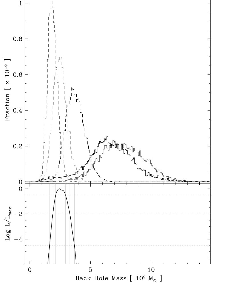
This maximum-likelihood estimate allows us to set a very secure $3\sigma$ lower limit on the mass of the black hole of $1.6\,10^{9}$ M_⊙. Using only the Balmer lines, we find a mass of $2.42\,10^{9}$ M_⊙, with $1\sigma$, $2\sigma$, and $3\sigma$ confidence intervals of $2.13-2.76\,10^{9}$ M_⊙, $1.86-3.08\,10^{9}$ M_⊙, and $1.58-3.45\,10^{9}$ M_⊙, respectively.

5 Discussion

5.1 Black-hole mass and Eddington ratio

The main result of this study is the discrepancy between the masses found by K00 and our estimates, since they differ by a factor ranging from 12 up to 60. As our study of the Balmer lines shows, discrepancies affect both the estimates of the delays and of the line widths. A general argument in favor of our mass estimate is the good qualitative agreement between the individual estimates for the Ly$\alpha$, Civ, and the three Balmer lines. The largest difference between the UV and Balmer lines is a factor three, while the systematics in the two sets of data can be quite different. By contrast, the K00 estimates, reported in Table 6, differ by a factor 5 between each other, and about $4.5$ for H$\alpha$ only, although all the estimates have been obtained with a consistent data set. In our study, we could not determine the rms profiles of the Balmer lines (not even their average profiles), because of the lack of data. Therefore, it is quite probable that a large part of the UV-Balmer discrepancy would be alleviated if the same methodology could be applied to the Balmer lines as well. It must be noted that all Balmer profiles are affected by contaminating emission lines, in addition to the narrow-line Balmer emission: [Nii] $\lambda$6548 and [Nii] $\lambda$6583 for H$\alpha$; [Oiii] $\lambda$4959 and [Oiii] $\lambda$5007 for H$\beta$; [Oiii] $\lambda$4363 for H$\gamma$. The [Oiii] lines being particularly strong in the wing of H$\beta$, its red profile had to be excluded from our analysis. The H$\beta$ region is moreover seriously contaminated by Feii pseudo-continuum emission (Boroson & Green 1992), making the line profile of H$\beta$ quite uncertain. The remaining narrow lines, plus the narrow-line Balmer emission, may significantly modify the true broad-line profiles. As they fall close to the Balmer line centers, their effect is to reduce the line second moments, providing underestimated black-hole masses. We thus conclude that, although affected by larger statistical errors, the UV-line estimates very probably suffer from smaller systematic errors. Therefore, the best mass estimate is the combined UV mass: $6.59\,10^{9}$  M_⊙, with a $3\sigma$ lower limit of $3.44\,10^{9}$  M_⊙. Including the Balmer lines, the $3\sigma$ lower limit is found to be $1.6\,10^{9}$ M_⊙. This lower limit is very robus, and should only increase if the systematic errors are reduced.

We point out that this fairly high mass estimate is obtained under the hypothesis that the gas motion is virialized and (close to) isotropic. As 3C 273 has a superluminal jet (e.g., Courvoisier 1998), 3C 273’s accretion disk is very probably close to face-on (assuming the disk is perpendicular to the jet), so projected velocities of particles in the disk would be greatly reduced by the geometry. If the emission lines originate from the disk, the mass estimate should be multiplied by a factor $1/\sin{i}>6$, if the angle between the perpendicular to the disk and the line of sight is $i<10^{\circ}$. On the basis of the response of the UV lines, we also concluded in Paper I that accretion-disk geometries of the broad line region can be excluded in this object.

Our comparison between the red and full profiles for the Ly$\alpha$ and Civ emission lines shows that inclusion of the possibly outflowing gas seen in Paper I would misleadingly increase the estimate of the mass of the black hole by approximately 15–30%. This is far from negligible, but it also shows that the order of magnitude of our result is not affected by the choice of using only the red profile.

From Courvoisier (1998) and Türler et al. (1999), we estimate the bolometric luminosity of 3C 273 to be approximately $10^{47}$ erg s^-1 (using $H_{0}\!=\!70$ km s^-1 Mpc^-1), giving an Eddington mass of about $10^{9}$ M_⊙. Using the 5100 Å flux as an estimate of the bolometric luminosity and a different cosmology, K00 find a comparable value of $\sim 0.5\,10^{9}$ M_⊙. According to the results of K00, the ratio between the mass derived from the Eddington luminosity and that from the reverberation method is therefore in the range 1–4, depending on which mass estimates are used, which makes 3C 273 a very strong candidate for super-Eddington accretion. Using our new reverberation-method mass, the Eddington ratio is estimated to be about $0.15$ and, using the individual estimates, falls in the range 0.13–0.53, i.e. in a fully sub-Eddington regime.

5.2 Size of the broad-line region

The size of the Balmer-emitting broad-line region in AGN has been investigated by several authors (Koratkar & Gaskell 1991a; Wandel et al. 1999, K00). While the first two studies find a BLR size $R_{\mathrm{BLR}}$ scaling roughly as $L^{0.5}$, K00 find a steeper relationship $R_{\mathrm{BLR}}\sim L^{0.700\pm 0.033}$ using a sample of 34 objects that were investigated using the reverberation method. The $L^{0.5}$ relationship is expected if gas density and ionization parameters are independent of the source luminosity in the emitting region. However, Vestergaard (2002) correctly points out that the K00 relationship is calculated with a method unable to take the strong intrinsic scatter into account, which produces biased slopes and too low uncertainties. Applying the BCES method of Akritas & Bershady (1996) on the K00 data and using a modified BLR size for NGC 4051 from Peterson et al. (2000), she found $R_{\mathrm{BLR}}\sim L^{0.58\pm 0.09}$, perfectly compatible with $L^{0.5}$. We can refine this relationship by using the new $R_{\mathrm{BLR}}$ for 3C 273 found in this work and by including new measurements for NGC 3783 (Onken & Peterson 2002), and NGC 3227 (Onken et al. 2003). 3C 273 has an important weight in the relationship, because it is the highest-luminosity object in the sample. From a maximum-likelihood estimator on the lag of the three Balmer lines, we have $R_{\mathrm{BLR}}=986^{+21}_{-37}$ days. Applying the BCES estimator, we obtain

$$R_{\mathrm{BLR}}\sim\lambda L_{\lambda}(5100\,\AA)^{0.59\pm 0.09}.$$ (6)

The two relationships are perfectly compatible with each other and still compatible with a $L^{0.5}$ relationship. Excluding NGC 4051 as proposed in Vestergaard (2002), the slope becomes $0.67\pm 0.10$, but it is not clear why this object should be discarded, as its distance to the BCES estimator does not appear unreasonable, considering its uncertainty. It must be noted, however, that this object has a very strong weight in the relationship.

McLure & Jarvis (2002) recalculated the $L_{\lambda}(5100\,\AA)$ luminosities using fluxes from Neugebauer et al. (1987) and a modern cosmology ($\Omega_{m}\!=\!0.3$, $\Omega_{\Lambda}\!=\!0.7$, $H_{0}\!=\!70$ km s^-1 Mpc^-1), and found a slope flatter than K00. We find here that, while the slope of the bisector is slightly lower, it is not significantly affected by the new luminosities, showing that the K00 luminosities are sufficiently accurate.

5.3 Mass-luminosity relationship

With the same sample, K00 investigated the mass-luminosity relationship in 34 Seyfert 1 and QSOs. They found that the relationship deviates significantly from the $L\sim M$ relationship, which is expected if the Eddington ratio $L_{\mathrm{bol}}/L_{\mathrm{Eddington}}$ is independent of the black-hole mass. They find $M_{\mathrm{BH}}\sim L^{0.5\pm 0.1}$, meaning that Seyfert 1 galaxies have low accretion rates compared to QSOs. It even strongly suggests that very luminous QSOs must accrete in the super-Eddington regime. This result has indeed sparked a lot of interest in the theoretical investigation of super-Eddington models (Collin et al. 2002).

As we find that 3C 273 has a lower accretion rate than previously thought, we reexplore the mass-luminosity relationship using the BCES bisector. With the new 3C 273 mass found here and the updated masses of the three Seyfert galaxies, we find

$$M_{\mathrm{BH}}\sim\lambda L_{\lambda}(5100\,\AA)^{0.65\pm 0.18}.$$ (7)

Figure 9 shows the updated mass-luminosity relationship.

Figure 9: Mass-luminosity for the 34 objects in the K00 sample. The solid line is the BCES bisector. The dashed line is the BCES bisector obtained after discarding unreliable objects. The shaded area shows the 1$\sigma$ error domain. The square, circle, triangle and pentagon respectively show 3C 273, NGC 4051, PG 1613+658, and PG 1704+608.

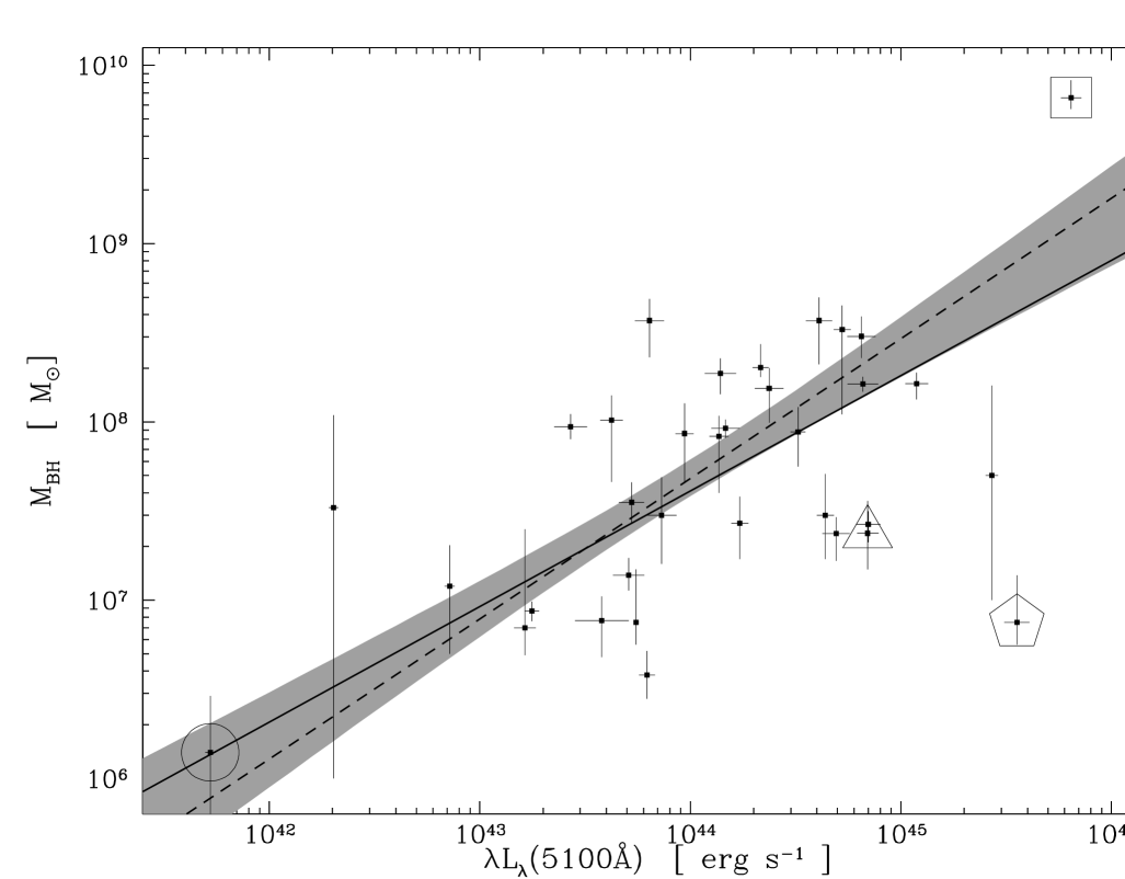
We caution, however, that this relationship can be disturbed by a few ill-measured masses. For instance, in the K00 sample two objects, PG 1613+658 and PG 1704+608, have masses differing by a factor 5 or larger, depending on whether the rms- or mean-profile method is used. If we discard these objects as too unreliable, we obtain

$$M_{\mathrm{BH}}\sim\lambda L_{\lambda}(5100\,\AA)^{0.79\pm 0.19}.$$ (8)

The reverberation-mass sample is therefore compatible with an Eddington ratio independent of the black-hole mass. This is consistent with the conclusion of Woo & Urry (2002), who investigated the mass-luminosity relationship in a sample of 377 AGN whose masses had been estimated using different methods, including reverberation. If the absence of relationship is confirmed, it means that there may currently be no need for super-Eddington-luminosity models.

Here as well, using the luminosities from McLure & Jarvis (2002) does not significantly affect the bisector estimates.

6 Conclusion

The most important consequence of this work is to show that the reverberation method can provide quite different results on a single object, as we find a black hole mass of about $6.59\,10^{9}$ M_⊙, an order of magnitude larger than in the previous study of K00. This result is considerably stronger than that of Krolik (2001), because it shows that serious discrepancies can result from the measurement of the delays and line widths and not only from the underlying assumptions of the method. In this study, we benefited from a much better determination of the delay between the lines and the continuum, thanks to the use of the ultraviolet continuum with a better sampling. However a large fraction of the discrepancy is caused by the determination of the line widths, for which we can propose only tentative explanations.

The mass determined from Balmer lines is about a factor 3 smaller than that obtained from the UV lines, but because of the lack of adequate data we could not determine the rms profile of the Balmer lines and had to rely on a less optimal velocity-dispersion measurement method. Thus at least part of the discrepancy can be explained by the different systematics and in particular by the inclusion of narrow-line emission in the line profile. Our Balmer-line mass is, in any case, at least a factor 5 larger than the previous study’s estimate. We are able to put a very robust $3\sigma$ lower limit on the mass of the black hole in 3C 273 of $1.6\,10^{9}$ M_⊙.

We studied the mass-luminosity relationship of supermassive black holes determined with the reverberation method. Using our new 3C 273 mass estimat, and updated estimates for three Seyfert galaxies, we find that the case for a correlation between the Eddington ratio and the black-hole mass in the reverberation-method sample is far from established.

We add finally that, in a very recent in-depth reanalysis of the exhaustive data set from the AGN Watch collaboration (Alloin et al. 1994), Peterson et al. (2004) obtained a new estimate of the mass of 3C 273 of $0.89\pm 0.19\,10^{9}$ M_⊙. Using our delay estimates for the Balmer lines, the estimated mass would be approximately $2.5\,10^{9}$ M_⊙, perfectly compatible with our own estimate using the Balmer lines ($2.42\,10^{9}$ M_⊙). Peterson et al. (2004) also give a much improved estimate of the slope of the mass-luminosity relationship $M_{\mathrm{BH}}\sim L^{0.79\pm 0.09}$, again in complete agreement with our work.