The proto–neutron–star dynamo — viability and impediments

We study convective motions taken from hydrodynamic simulations of rotating proto–neutron stars (PNSs) with respect to their ability to excite a dynamo instability which may be responsible for the giant neutron star magnetic fields. Since it is impossible to simulate the magnetic field evolution employing the actual magnetic Reynolds numbers ($\operatorname{\mathit{Rm}}$) resulting from the hydrodynamic simulations, (smallest) critical $\operatorname{\mathit{Rm}}$s and the corresponding field geometries are derived on the kinematic level by rescaling the velocity amplitudes. It turns out that the actual values of $\operatorname{\mathit{Rm}}$ are by many orders of magnitude larger than the critical values found. A dynamo might therefore start to act vigorously very soon after the onset of convection. But as in general dynamo growth rates are non–monotonous functions of $\operatorname{\mathit{Rm}}$ the later fate of the magnetic field is uncertain. Hence, no reliable statements on the existence and efficiency of PNS dynamos can be drawn without considering the interplay of magnetic field and convection from the beginning. Likewise, in so far as convection inside the PNS is regarded to be essential in re–launching the supernova explosion, a revision of its role in this respect could turn out to be necessary.

1 Introduction

The origin of the neutron star (NS) magnetic fields is subject of scientific debate since the discovery that the pulsar mechanism is based on the existence of the strongest magnetic fields seen in the universe. Though the idea of magnetic flux conservation during the collapse of the NS progenitor came up quite naturally, doubts as to whether that mechanism explains the observed field strengths were raised almost simultaneously (see, e.g., Thompson & Duncan, 1993). That macroscopic currents – as almost everywhere else in the universe – are the cause of the NSs’ magnetic fields seemed obvious; thus attention has been drawn to the idea of a dynamo. Flowers & Ruderman (1977) first pointed out that such an instability can start to act immediately after the neutron star’s birth, and last until its internal motions disappear.

The increasing understanding of the supernova mechanism (e.g., Burrows & Fryxell, 1992, and references therein) and the accompanying process of NS creation strengthened the idea of a convective proto–neutron star (PNS) phase. This very first epoch in a NS’s life starts immediately after the collapse when negative radial gradients of both entropy and lepton number are created, thus in general enabling Ledoux convection (see, e.g., Epstein (1979) and Burrows & Lattimer (1986)) and lasts about half a minute. Thompson & Duncan (1993) sketched the possibility of dynamo action caused by turbulent convective motions in the PNS. They claimed that as these vigorous motions combine with differential rotation, a mean–field dynamo of $\alpha$–$\Omega$ type may act in regions where the rotation is capable of influencing the convection significantly. By use of a mixing–length approach they estimated the convective velocity to be about $10^{8}$ cm s^-1 and concluded from equipartition that such a dynamo may amplify a seed field up to $10^{15}$G during the first $30$ seconds of a NS’s life. In contrast, small–scale dynamo action without generation of a coherent large–scale field should be expected where the influence of the rotation on the convection is negligible.

In two complementary papers, Bonanno et al. (2003) and Urpin & Gil (2004) recently presented studies on field generation in PNSs where the former deals with mean–field dynamos and the latter with small–scale ones.

In their strongly simplified model, Bonanno et al. (2003) assume the mean e.m.f. to be constituted by isotropic $\alpha$ and $\beta$ effects only and adopt purely radial dependences for differential rotation, the $\alpha$–parameter and the turbulent magnetic diffusivity. Like Thompson & Duncan (1993) and based on the results of Miralles et al. (2002), they argue that $\alpha$ is negligible in an inner, entropy–gradient driven convective region, but proportional to the rotation rate $\Omega$ in an overlaying, lepton–gradient driven convective shell. They derive critical values of $\Omega$ above which dynamo action in either the $\alpha^{2}$ or the $\alpha$–$\Omega$ regime is possible and conclude that the vast majority of PNSs will show mean–field dynamo action.

The work of Urpin & Gil (2004) is focused on small–scale dynamos which are supposed to emerge from both convective regions. As the magnetic Reynolds numbers are huge even when calculated with the scales of the convective eddies, at least a necessary condition for this supposition is surely satisfied. To get estimates for the magnetic field strength at the end of the convective phase, equipartition is employed thus arriving at magnetic field strengths of $\approx 10^{13}$G in both convective regions for the largest turbulent scales $\approx 1\,\ldots\,3$ km.

Both studies state that given the estimated convection amplitudes, dynamos can act because the velocities are overcritical with respect to these dynamos. Urpin & Gil (2004) do not estimate the real level of ‘overcriticality’, i.e. the ‘distance’ between the real and the critical velocity (e.g. as a ratio of amplitudes) at all. Bonanno et al. (2003) provide a hint that in terms of the mean–field coefficient $\alpha$ the real flow might be overcritical by a factor up to 1000 but refrain from discussing the consequences on the basis of the behavior of growth rates.

But, as in general the growth rates do not simply grow with growing overcriticality (in the above sense) no reliable conclusion on dynamo action can be drawn without calculating them based on realistic velocity amplitudes. Moreover, it appears desirable to overcome the drawback of using ad–hoc assumptions on the convection and instead to make use of ‘realistic’ convective velocity patterns obtained from hydrodynamic simulations of the PNS stage. By feeding them into dynamo calculations ‘as they are’, a better understanding of the different PNS layers’ contributions to the field generation and hence the relative importance of small and large–scale dynamos could be gained.

Along with the problem of magnetic field generation, the comparatively short period of convection in PNSs has been taken to play an important role in the puzzle of another major question: How can a sufficiently large amount of heat and/or neutrinos be transported into the region behind the shock front to enable the re–energized supernova explosion?

Recently, doubts have been reinforced about whether the PNS convection alone is sufficient to accomplish this and new hints have been provided that convection in a second outer spherical shell (50 ​…100 km) could be crucial instead (see Janka et al., 2004, and references therein). But at least in the case when the thermal energy stored outside the neutrinosphere and transported by this convection towards the shock is not sufficient to re–launch it, the transport of neutrinos trapped inside the neutrinosphere by virtue of the coupled action of the inner (PNS) and outer convective zones could help: If the overshooting zone of the former and the undershooting zone of the latter overlap, a sufficient number of neutrinos would be enabled to escape from the PNS and to reach the post-shock heating zone.

Up to now, all attempts to cope with the problem of the convection–driven explosion were made with the influence of the magnetic field neglected. But, if success or failure depends sensitively on details of the convective phase, a clear understanding of how early and how fast the magnetic field starts to act back on the motions which generated it (perhaps in both convection zones) seems to be essential. Miralles et al. (2002) were the first to include the influence of an imposed magnetic field on the conditions for the onset of the relevant convective instabilities and found that only extremely strong ($10^{15}$G) magnetic fields suppress the occurrence of convection completely.

Since the mid–nineties fully nonlinear hydrodynamic supernova simulations also resolving the PNS started to provide more detailed insight into the convection there (see, e.g., Keil, 1997; Janka & Keil, 1998; Fryer & Heger, 2000; Janka, 2004; Janka et al., 2004).

2 Kinematic dynamo action of PNS convection

The purpose of this paper is to study the dynamo–related properties of velocity profiles found in hydrodynamic PNS simulations. To start with, we restrict ourselves to the kinematic approach, that is, we solve the induction equation with prescribed velocities $v$. It reads in normalized form for a homogeneous medium

$$\dot{{\mbox{\boldmath$B$}}}=\operatorname{\Delta}{\mbox{\boldmath$B$}}+\operatorname{\mathit{Rm}}\operatorname{curl}({\mbox{\boldmath$v$}}\times{\mbox{\boldmath$B$}})\,,\quad\operatorname{div}{\mbox{\boldmath$B$}}=0$$ (1)

where $\operatorname{\mathit{Rm}}=UR/\eta$ is the magnetic Reynolds number with a characteristic velocity $U$, the magnetic diffusivity $\eta$ and the radius $R$ of the PNS. We define $v$ by snapshots taken from the simulations of Keil (1997) (see also Janka & Keil, 1998) who performed 2D (axisymmetric) simulations of rotating PNS convection with a model including a completely radial neutrino transport scheme and employing the EOS of Lattimer and Swesty without accretion. To check both an early stage possibly relevant for the explosion and a stage with fully developed convection perhaps determining the later NS field, we took the velocity profiles at $30$ ms and $0.9$ s after bounce.

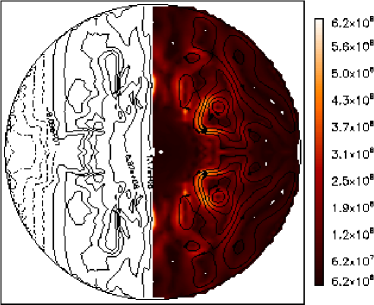
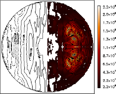
Figure 1: Convective velocities simulated by Keil (1997) for $30$ ms (left) and $0.9$ s (right) after bounce in cm s^-1. In the left semicircles the isolines of the azimuthal velocity and in the right ones the streamlines of the meridional velocity are shown. Note that the former is measured with respect to a frame in which the flow has zero angular momentum. In the right semicircles background colors provide the modulus of the meridional velocity.

The geometrical structures of the convective velocities $\@vec{v}$ are shown in Fig. 1; Table 1 summarizes their main qualitative features. At the late stage the azimuthal velocity component (i.e., the differential rotation) is in a large portion of the PNS’s volume nearly independent of $z$, as a consequence of the Taylor–Proudman theorem. The early velocity pattern is dominated by only a few convective cells per hemisphere whereas the late one shows more and, hence, smaller cells.

Table 1: Qualitative features of the convective velocities: $R$ - PNS radius, $R_{\text{i}},R_{\text{o}}$ - estimated inner and outer radii of the convective shell; $N_{\theta}$, $N_{r}$ - number of prominent convective cells in meridional and radial directions; $v_{\text{max}}$ - maximum convective, $v^{\text{merid}}_{\text{max}}$ - maximum meridional velocity. $\operatorname{\mathit{Rm}}$ - magnetic Reynolds number based on the r.m.s. value of the velocity with respect to the full PNS volume and an electric conductivity of $10^{24}\mbox{s}^{-1}$.

	30 ms	0.9 s
$R$ (km)	59	22
$R_{\text{i}}/R$	0.3	0.5
$R_{\text{o}}/R$	0.75	0.78
$N_{\theta}$	2	8
$N_{r}$	1	2
$v_{\text{max}}$ (cm/s)	$1.3\cdot 10^{9}$	$2.2\cdot 10^{9}$
$v^{\text{merid}}_{\text{max}}$(cm/s)	$6.3\cdot 10^{8}$	$2.2\cdot 10^{8}$
$\operatorname{\mathit{Rm}}$	$4.2\cdot 10^{19}$	$2.2\cdot 10^{19}$

As the velocity patterns are reflectionally symmetric with respect to the equatorial plane and symmetric about the PNS’s axis of rotation, any eigensolution of (1) is either equatorially symmetric (S) or antisymmetric (A) and its spherical components vary like $\cos m\varphi$ or $\sin m\varphi$, $m=0,1,2,\ldots$ where $\varphi$ is the azimuth with respect to the rotation axis. For non–decaying solutions the case $m=0$ (axisymmetry) is excluded by Cowling’s theorem. As a consequence, if dipolar dynamo solutions, i.e. in our case, S1–solutions, occur their axes are bound to lie in the equatorial plane. Note that this restriction is only due to the axisymmetry of $v$ and does not apply to a realistic situation with 3D convection. Then, it is well possible that a dominating axisymmetric (aligned) dipolar field, accompanied by non–axisymmetric constituents is generated. We restrict ourselves here to the case $m=1$ only as from experience we expect those modes to be the most easily excitable ones. Both equatorial symmetries are included, that is, for either velocity the A1 and S1 solutions are considered.

For the boundary conditions at the surface we assumed the surroundings of the PNS to exhibit a significantly lower electric conductivity than its interior. We modeled this condition by requiring that the magnetic field is at the surface continued into a vacuum field.

As we cannot hope to solve Eq. (1) with the velocity snapshots’ real values of $\operatorname{\mathit{Rm}}$ (see Table 1) we restrict ourselves instead to determining the so–called critical values of $\operatorname{\mathit{Rm}}$, $\operatorname{\mathit{Rm}}_{\text{crit}}$, for which the total magnetic field energy (or a suitable temporal average of it) neither grows nor decays. The corresponding magnetic field solution is then called marginal. To accomplish this, the magnitude of the velocity was considered freely rescalable while its geometry remained fixed. That is, we simply multiplied the complete velocity field with a factor which was adjusted such that a marginal solution emerged. In mathematical terms, we sought solutions of Eq. (1) with an exponential ansatz for the time dependence of $B$, i.e., $\partial/\partial t=\lambda$, where the real part of the time increment $\lambda$ has to vanish. In general, this is not equivalent with stationarity of the marginal solutions as a non-vanishing imaginary part of $\lambda$ may occur causing oscillating marginal solutions. In our situation, however, in which we excluded axisymmetric ($m=0$) solutions, the oscillations introduced in this way are restricted to uniform rotations of the field pattern about the axis of rotation, where the imaginary part $\Im\{\lambda\}$ defines the rotation rate. Hence, the magnetic field energy is for any marginal solution a constant quantity.

Our actual technique to determine $\operatorname{\mathit{Rm}}_{\text{crit}}$ together with the corresponding marginal solution was to integrate (1) as an initial value problem. We started with values of $B$ specified according to the desired symmetry type (A1 or S1) of the solution, but arbitrary otherwise. In every time step we adjusted $\operatorname{\mathit{Rm}}$ (automatically) such that the total magnetic energy approached a stationary value. As no marginal solutions exist for which the total magnetic energy is oscillating no modes of a given symmetry type can be overlooked the $\operatorname{\mathit{Rm}}_{\text{crit}}$ of which could possibly be smaller than the detected one.

We used a spectral code based on the magnetic field’s free decay modes, specified for vacuum boundary conditions. Each of these modes is characterized by a spherical harmonic $Y_{l}^{m}(\vartheta,\varphi)$ providing the angular dependence and a spherical Bessel function $j_{l}(\mu_{ln}r)$ providing the radial one ($r,\vartheta,\varphi$ - spherical co–ordinates). Here, $\mu_{ln}^{2}$ is the corresponding decay rate with $n$ giving roughly the number of zeros between center and surface of the PNS.

Table 2 summarizes the critical magnetic Reynolds numbers $\operatorname{\mathit{Rm}}_{\text{crit}}$ for the different velocities and field types and some characteristic properties of the marginal magnetic eigensolutions, which are all non–oscillatory, that is, $\Im\{\lambda\}=0$.

Table 2: Critical magnetic Reynolds numbers and characteristics of the marginal eigensolutions for the velocities considered. $E_{\text{pol}}$ and $E_{\text{tor}}$ are the energies of the poloidal and toroidal parts of the field, respectively, where the poloidal part comprises the externally observable multipole constituents. The toroidal field is zero outside the PNS and its field lines lie completely in spherical surfaces. $(l,n)_{\text{max}}$ are the maximum spherical harmonic order and number of radial zeros, respectively, included in the numerical model; $(l,n)_{\text{dom}}$ correspond to the scales dominating in the energy spectra of the solutions.

	30 ms		0.9 s
	A1	S1	A1	S1
$\operatorname{\mathit{Rm}}_{\text{crit}}$	4077	4021	8720	6007
$E_{\text{pol}}/E_{\text{tor}}$	0.24	0.27	0.03	0.11
$l_{\text{max}}$	121	121	120	121
$n_{\text{max}}$	70	70	66	70
$l_{\text{dom}}$	13	12	3	1
$n_{\text{dom}}$	2	2	9	3

In Figs. 2 and 3 we present these magnetic fields on the surface of the PNS and on a spherical surface inside the convective shell where field generation is supposed to be most vigorous. Note that the A1 solutions contain quadrupoles, but those without any axis of symmetry ($Y_{2}^{1}(\vartheta,\varphi)$). We emphasize that the magnetic fields shown belong to velocity fields extracted from the evolution of the PNS convection and then considered fixed, i.e., the fields corresponding to the later moment has not evolved from the one corresponding to the earlier.

In their spherical harmonic spectra (referring to latitudinal scales), the ‘late’ magnetic fields show somewhat larger scales than the ‘early’ ones, but smaller scales in their spherical Bessel spectra (referring to radial scales). Both S1 fields are at the surface predominant around the equator where the early field has its maxima while the maxima of the late one occur at $\pm 30^{o}$.

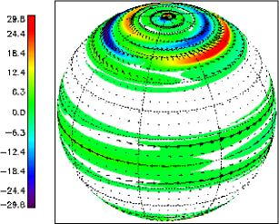
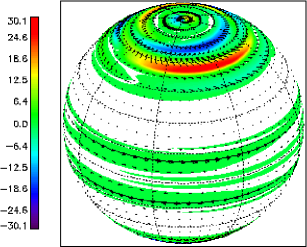
Figure 2: Marginal dynamo fields for the velocity from the model of Keil (1997) at 30 ms after bounce. Left: S1, right A1 solution. Upper row: $r=R$, lower row $r=0.5R$. Arrows: tangential components, color encoding: normal component. The field strengths are arbitrary as Eq. (1) is linear and homogeneous.

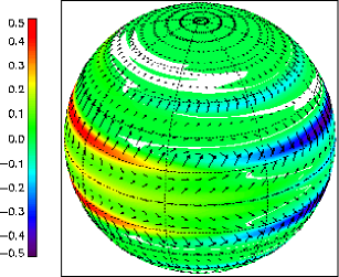
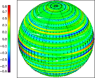
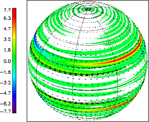
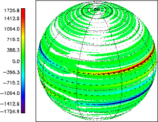
Figure 3: The same as Fig. 2, but for the velocity at 0.9 s after bounce. Here, the radius of the inner surface (lower row) is $r=0.6R$.

3 Conclusions

The main conclusion to be drawn is that the geometrical structures of the velocity fields employed are well suited to amplify a magnetic seed field. However, given the huge electric conductivity of the PNS matter ($\approx 10^{24}\mbox{s}^{-1}$, see, e.g., Thompson & Duncan (1993), Table 1) and convective velocities of $\approx 10^{8}$cm s^-1, the magnetic Reynolds numbers turn out to be by about 16 orders of magnitude overcritical. As in general there is no monotonous relation between the growth rate of a dynamo and $\operatorname{\mathit{Rm}}$ nothing can thus be inferred with certainty about the dynamo activity of the considered convective flows at their given strengths. However, it is known that due to increasing flux expulsion the growth rate as a function of $\operatorname{\mathit{Rm}}$ will typically reach a maximum and then decrease until the dynamo–ability of the flow may get lost completely or at least the growth rate approaches zero (‘slow dynamo’). [See, e.g., Fuchs et al. (1997) for the Gubbins flow, where the ratio of the upper to the lower critical $\operatorname{\mathit{Rm}}$ for the $m=1$ modes is only 5, or Rädler et al. (2002) where it is shown that the $\alpha$ coefficient of the mean–field model of the Karlsruhe dynamo experiment decreases with growing fluid velocity.]

There is no way to calculate magnetic field growth rates with the velocity amplitudes given above, as all experience shows that the field scales get smaller and smaller with growing $\operatorname{\mathit{Rm}}$. In our case, we are sure that with the available computing resources the necessary spatial resolution is by far unreachable. Even if the problem would perhaps be less difficult in ideal MHD, one has to be aware that then the Bondi–Gold theorem prohibits a kinematic dynamo solution unequal to zero outside the PNS.

On the other hand, PNS convection is a transient phenomenon starting from small amplitudes and ending with the fluid at rest. Let us discuss the possible scenarios assuming that the convection starts with a sufficiently small $\operatorname{\mathit{Rm}}$ and then passes, continuously growing, through a stage which is critical with respect to the dynamo.

First we assume that all stages of the convection beyond that point and up to a second critical stage only close to the very end of the convective phase show positive growth rates of the corresponding kinematic dynamos. Then, a magnetic field will be generated anyway (see Fig. 4, case (i)) .

In a contrasting scenario, the increasing convection could leave its dynamo–active phase very soon after having entered it (see Fig. 4, case (ii)). Then again two possibilities exist: If the magnetic field grows so slowly that it cannot influence the flow significantly before it loses its dynamo–capability again, no strong fields will be generated and the vigorous convection can even destroy the (weak) field it had begun to build up before (see Fig. 4, case (iia)). In the opposite case, the magnetic field grows so fast that its Lorentz forces become able to hinder the convection from reaching amplitudes too high for dynamo action (see Fig. 4, case (iib)). That is, the generated field could fundamentally change the flow in a very early stage.

In the first case of the second scenario, a further option is the recovery of the dynamo ability of the convection during its dying-out. Then, the period during which the growth rate of the field is positive will be very short, limiting the accessible magnetic field strengths already on the kinematic level (see Fig. 4, case (iib)).

When accepting that the second scenario — the convection is a ‘slow dynamo’ — is the more probable one as ‘fast dynamos’ (growth rate positive and not approaching zero for $\operatorname{\mathit{Rm}}\rightarrow\infty$) are rarely found, we must either question the existence of an efficient PNS dynamo or declare that the influence of the generated magnetic field must not be neglected. Consequently, the possible essential role of PNS convection in enabling the supernova explosion must then be revised given its significant modification by the magnetic field at a very early stage. The only way to decide between the expounded alternatives is to perform MHD–calculations starting from the very beginning of the convection, i.e., with extremely small velocities.

We concede, that the two major scenarios (cases (i) and (ii) in Fig. 4) represent only the extrema of an infinitude of possibilities which could be constructed when assuming rapid changes in the dynamo–related properties of the convection during its lifetime: Already for a fixed flow geometry the dynamo growth rate $p$ as a function of $\operatorname{\mathit{Rm}}$ may change its sign several times in the relevant range of values. But as the flow geometry is not fixed during the lifetime of the convection, even its characterization as a slow or fast dynamo could be different at different moments. Nevertheless, for any time interval with a positive $p$ terminated by a sign change of $p$ the discussion summarized as cases (iia) and (iib) can be applied likewise leading again to the above crucial alternative. Of course, possible consequences for the role of PNS convection in supporting SN explosions can only be expected during (roughly) the first second of the PNS’s life.

Assumption:

dynamo growth rate $p>0$

immediately after onset

of PNS convection

Case (i):

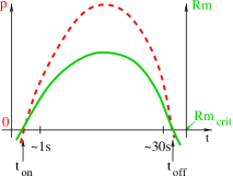
“fast dynamo” $\longrightarrow$ magnetic field generation for all $t_{\text{on}}\leq t\leq t_{\text{off}}$

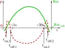
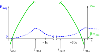
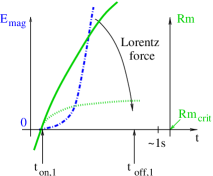
Case (ii): “slow dynamo” $\longrightarrow$ back–reaction of $B$ on convection crucial for magnetic field evolution Case (iia): convection not affected by $B$ $\longrightarrow$ no strong $B$ possible Case (iib): convection affected by $B$ $\longrightarrow$ $Rm\,$ values inhibiting dynamo not reached $\longrightarrow$ strong $B$ possible

Figure 4: Schematic representation of possible PNS dynamo scenarios. $\operatorname{\mathit{Rm}}$ – magnetic Reynolds number (solid and dotted [lower right panel]/green); $p=\Re\{\lambda\}$ – dynamo growth rate (dashed/red); $E_{\text{mag}}$ – energy of the entire PNS magnetic field (dash-dot/blue). Colors refer to the online version. Note that the curves for $\operatorname{\mathit{Rm}}$, $p$ and $E_{\text{mag}}$ are sketched as if no back–reaction of the magnetic field on the convection existed (exception: dotted curve in lower right panel).