The case for a distributed solar dynamo shaped by near-surface shear

Abstract

Arguments for and against the widely accepted picture of a solar dynamo being seated in the tachocline are reviewed and alternative ideas concerning dynamos operating in the bulk of the convection zone, or perhaps even in the near-surface shear layer, are discussed. Based on the angular velocities of magnetic tracers it is argued that the observations are compatible with a distributed dynamo that may be strongly shaped by the near-surface shear layer. Direct simulations of dynamo action in a slab with turbulence and shear are presented to discuss filling factor and tilt angles of bipolar regions in such a model.

1. Introduction

There appears to be general consensus that the solar magnetic field is generated and stored in the overshoot layer near the bottom of the convection zone (Spiegel & Weiss 1980, Golub et al. 1981, Galloway & Weiss 1981, van Ballegooijen 1982, Choudhuri 1990). This layer is now believed to coincide with the tachocline, i.e. the radial shear layer at the bottom of the convection zone where the latitudinal differential rotation changes into rigid rotation in the radiative zone (Spiegel & Zahn 1992). The main arguments in favor of this proposal are connected with flux storage over times long enough for the shear to amplify the toroidal field (Moreno-Insertis, Schüssler, & Ferriz-Mas 1992), and with the observed size of active regions ($\sim 100\,{\rm Mm}$) being comparable with the typical eddy scale at the bottom of the convection zone (Galloway & Weiss 1981), as well as the observed fidelity of Hale’s polarity law; see Fisher et al. (2000), Tobias (2002), Schüssler (2002), Ossendrijver (2003), Fan (2004), and Weiss (2005) for recent reviews. All these aspects are intimately related to the thin flux tube picture. Indeed, one of the big successes of the thin flux tube approximation (Spruit 1981, Moreno-Insertis 1986, Chou & Fisher 1989) is the quantitative prediction of Joy’s law describing the latitudinal dependence of the observed tilt angles of bipolar regions. It is found that Joy’s law is obeyed only for flux tubes with magnetic fields that are of the order of $10^{5}\,{\rm G}$ (D’Silva & Choudhuri 1993, Schüssler et al. 1994, Caligari, Moreno-Insertis, & Schüssler 1995). This result poses rather stringent demands on dynamo theory that are hard to meet. Although it may already be hard for the differential rotation in the tachocline to amplify a poloidal field to a strength of $\sim 10^{5}\,{\rm G}$, which may require flux intensification by exploding flux tubes (Rempel & Schüssler 2001), it is not obvious how to explain the production of strong and sufficiently coherent poloidal field that is necessary to produce the toroidal field.

The purpose of the present paper is to discuss the difficulties for dynamo theory in meeting these demands and to reconsider the alternative scenario that the solar dynamo may operate in the bulk of the convection zone, or perhaps even in the near-surface shear layer in the upper $35\,{\rm Mm}$ of the sun. This is the layer where recent helioseismological inversions have shown marked negative radial shear (Howe et al. 2000a, Corbard & Thompson 2002, Thompson et al. 2003). The presence of a deeper layer that spins about 5% faster than the photosphere has always been anticipated based on the higher rotation rate of magnetic tracers (Gilman & Foukal 1979, Golub et al. 1981). It remained unclear, however, just how deep or shallow this layer really is. The most natural assumption at the time was to place this layer near the bottom of the convection zone where magnetic buoyancy is weak and shear could work on the field unimpeded by the turbulence. In the early days of mean field dynamo theory a negative radial $\Omega$ gradient was already anticipated (Stix 1976, Yoshimura 1976) because it would explain the observed anticorrelation of the signs of mean azimuthal field (inferred from the orientation of bipolar regions) and the mean radial field (measured by magnetograms). This is because negative radial shear turns a positive radial field into a negative azimuthal field, producing the observed anticorrelation. A negative radial gradient of angular velocity seemed confirmed by observations of very young sunspots that rotate faster than older ones (Tuominen 1962), suggesting that they may be anchored in the layer where the angular velocity is maximum (Tuominen & Virtanen 1988, Balthasar, Schüssler, & Wöhl 1982, Nesme-Ribes, Ferreira, & Mein 1993, Pulkkinen & Tuominen 1998).

The sunspot observations are not easily explained by interface dynamos, unless one is able to show that the angular velocity of magnetic tracers is just the pattern speed of a traveling wave phenomenon. A similar proposal has been made to explain the observed pattern speed of the supergranulation (Gizon, Duvall, & Schou 2003, Schou 2003, Busse 2004).

The importance of the near-surface shear layer has already been investigated by Dikpati et al. (2002) who studied the effects of near-surface radial shear on a flux transport dynamo. They came to the conclusion that the effect of the near-surface shear layer is subdominant in the context of the flux transport model studied earlier by Dikpati & Charbonneau (1999). Mason, Hughes, & Tobias (2004) also considered the issue of near-surface dynamo action in the context of a two-layer dynamo (one at the top and one at the bottom of the convection zone). They allowed for an additional $\alpha$ effect in the upper layers, retaining only the radial shear in the tachocline. They came to the conclusion that the near-surface dynamo was harder to excite due to the larger distance to the tachocline.

There are several arguments in favor of a dynamo operating in or being strongly controlled by the near-surface layer of the sun. First, in the outer $35\,{\rm Mm}$ (corresponding to fractional radii $r/R\geq 0.95$) the negative radial shear, together with an $\alpha$ effect of the usual sign, would easily explain the observed equatorward migration of sunspot activity (e.g. Parker 1979). Second, the negative phase relation between radial and azimuthal mean fields, $\overline{B}_{r}$ and $\overline{B}_{\phi}$, respectively, would be automatically satisfied (Stix 1976, Yoshimura 1976). Third, the radial near-surface shear is particularly strong between the equator and $30^{\circ}$ latitude, and weak near the poles; see Fig. 1. In the tachocline, by contrast, there is hardly any radial shear at $30^{\circ}$ latitude and maximum shear near the poles. Invoking near-surface shear for producing sunspot activity would naturally explain the strongest production of sunspot activity at low latitudes and the much weaker magnetic activity at high latitudes with a possible poleward migration (Stix 1974), provided the near surface shear changes sign at high latitudes, as is perhaps indicated by helioseismology (Thompson et al. 2003). [The poleward branch could also be due poleward flows – as demonstrated convincingly by flux transport models; see Baumann et al. (2004) and Schüssler (2005).] Fourth, the rotational velocity of very young sunspots (age less than 1.5 days) is $14.7^{\circ}/{\rm day}$ at low latitudes (Pulkkinen & Tuominen 1998), corresponding to $473\,{\rm nHz}$, which is about the largest angular velocity measured with helioseismology anywhere in the sun; cf. Fig. 1. This corresponds to the angular velocity at a radius $r/R=0.95$, which is $35\,{\rm Mm}$ below the surface. Similar conclusions can be drawn from the apparent angular velocity of old and new magnetic flux at different latitudes (Benevolenskaya et al. 1999). We will return to these observations in §3.

The main argument against distributed and near-surface shear layer dynamos is that magnetic flux tubes are highly buoyant in the convection zone proper (Parker 1975). Thus, too much magnetic flux may be lost, on time scales so short that the shear cannot amplify the poloidal field to significant field strengths. However, over the past 15 years simulations have shown that magnetic buoyancy is strongly offset by the action of turbulent pumping, which leads to a net accumulation of magnetic energy at the bottom of the convection zone (Nordlund et al. 1992, Brandenburg et al. 1996, Tobias et al. 1998, 2001, Dorch & Nordlund 2001, Ossendrijver et al. 2002, Ziegler & Rüdiger 2003). Indeed, magnetic pumping is now also being invoked to keep down the horizontal magnetic fields just outside the penumbra of sunspots (Thomas et al. 2002, Weiss et al. 2004). Thus, we can envisage pumping as a mechanism that tries to keep the surface clean of magnetic fields, but it can do so only approximately and only if the field is not already too strong.

Another argument against near-surface dynamos is the high degree of turbulence in the upper layers, which could lead to strong random distortions of the orientation of flux tubes. This leads to the notion of rising flux tubes being ‘brain washed’ during their ascent (Schüssler 1983, 1984), i.e. they lose their original east-west orientation and would not obey Hale’s polarity law. However, this picture derives originally from the idea that flux tubes are produced in deep layers at or below the overshoot layer and are then subjected to a more passive buoyant rise through the convection zone. Here, however, we are envisaging the production of sunspots much closer to the surface, so the notion of flux tubes rising through a major portion of the convection zone is not invoked. Indeed, local helioseismology suggests a picture quite compatible with sunspots being a shallow surface phenomenon (Kosovichev, Duvall, & Scherrer 2000, Kosovichev 2002). The actual sunspot formation might then be the result of convective collapse of magnetic fibrils (Zwaan 1978, Spruit & Zweibel 1979), possibly facilitated by negative turbulent magnetic pressure effects (Kleeorin, Mond, & Rogachevskii 1996) or by an instability (Kitchatinov & Mazur 2000) causing the vertical flux to concentrate into a tube.

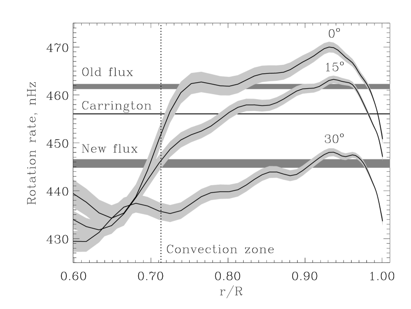
Figure 1.— Radial profiles of the internal solar rotation rate, as inferred from helioseismology. The angular velocities of active zones at the beginning of the cycle (at $\approx 30^{\circ}$ latitude) and near the end (at $\approx 4^{\circ}$) is indicated by horizontal bars, which intersect the profiles of angular velocity at $r/R\approx 0.97$. [Adapted from Benevolenskaya et al. (1999).]

It should be noted that the picture of shallow sunspots does not necessarily contradict the idea of strong flux tubes rising to the surface. In fact, as the tube rises to the surface, it must eventually undergo catastrophic expansion (Moreno-Insertis, Caligari, & Schüssler 1995). This would detach the forming active region and its sunspots from its roots (Schrijver & Title 1999, Schüssler 2005), which might then be compatible with the shallow sunspot picture from local sunspot helioseismology.

Yet another potential problem with near-surface shear layer dynamos are the relatively short turbulent time scales. However, in 35 Mm depth the typical turnover time is, according to mixing length theory (Spruit 1974), already 1–3 days. Therefore the inverse Rossby number, $2\Omega\tau$, is of the order of unity, so the turbulence is certainly beginning to be affected by rotation. As is familiar from mean field dynamo theory, the combination of poloidal and toroidal fields really corresponds to a right-handed spiral in the northern hemisphere. Thus, whenever parts of this spiral touch the surface they produce a bipolar active region with the observed tilt angle. This will be discussed further in §4.4.

We now turn to the question of small scale magnetic fields. For magnetic Prandtl numbers as small as those in the sun, the magnitude of the turbulent magnetic fields from local small scale dynamo action at the top of the convection zone (Cattaneo 1999) is possibly not much stronger than the magnitude of fields from the large scale dynamo. This suggestion is motivated by the recent realization that small scale dynamo action (as originally explored by Kazantsev 1968) becomes either completely impossible or at least much harder to excite when the magnetic Prandtl number becomes small (Schekochihin et al. 2004a, Boldyrev & Cattaneo 2004, Haugen, Brandenburg, & Dobler 2004). The dominance of small scale over large scale dynamo activity in global simulations of solar-like convection (Brun, Miesch, & Toomre 2004) might therefore also be related to the fact that the magnetic Prandtl number is not small in those simulations.

Another important aspect is the fact that in the presence of shear, turbulent dynamos can produce and maintain fields of equipartition strength (Brandenburg et al. 2005). We will discuss some of those models also in §4. Although such models still lack important aspects of solar dynamos (convection, stratification, and rotation), they are quite suitable for testing new effects in mean field theory, for example the shear–current effect (Rogachevskii & Kleeorin 2003, 2004) and current helicity fluxes (Brandenburg & Sandin 2004, Subramanian & Brandenburg 2004). We begin by discussing first the problems associated with the current picture of dynamos operating in the tachocline. A summary of arguments discussed in the text is given in Table 1.

Table 1Summary of arguments for and against tachocline and distributed dynamos discussed in the text

arguments	tachocline dynamos	distributed/near-surface dynamos
in favor	flux storage	negative surface shear yields equatorward migration
	turbulent distortions weak	correct phase relation
	correct butterfly diagram with meridional circulation	strong surface shear at latitudes where the spots are
	size of active regions ($\sim 100\,{\rm Mm}$) naturally explained	$\max(\Omega)/2\pi=473\,{\rm nHz}$ agrees with $\Omega(\mbox{youngest spots})$
		active zones move with $\Omega(0.95)$
		$11\,{\rm yr}$ variation of $\Omega$ seen in the outer $70\,{\rm Mm}$
		even fully convective stars have dynamos
against	$100\,{\rm kG}$ field hard to explain	strong turbulent distortions
	flux tube integrity during ascent	rapid buoyant losses
	too many flux belts in latitude	too many flux belts if dynamo only in shear layer
	maximum radial shear at the poles	not enough time for shear to act
	no radial shear where sunspots emerge	long term stability of active regions
	quadrupolar parity preferred	profile of $\Omega(\mbox{youngest})$ by $4\,{\rm nHz}$ above $\Omega(0.95)$
	wrong phase relation	possible anisotropies in supergranulation
	$1.3\,{\rm yr}$ instead of $11\,{\rm yr}$ variation of $\Omega$ at base of CZ
	coherent meridional circulation pattern required

2. Problems with tachocline dynamos

By tachocline dynamos we mean dynamos where the main shear that is responsible for the cyclic toroidal fields originates from the tachocline. These dynamos take into account the measured differential rotation profile, although sometimes the latitudinal shear is neglected (e.g. Parker 1993, Choudhuri, Schüssler, & Dikpati 1995). Tachocline dynamos can be divided into three main subclasses: (i) overshoot dynamos where there is only a negative $\alpha$ effect in the overshoot layer, (ii) interface dynamos where a negative $\alpha$ effect is assumed in the upper parts of the convection zone, and (iii) Babcock-Leighton type flux transport dynamos where the $\alpha$ effect is also located near the surface, but it is now positive and there is meridional circulation transporting flux in the overshoot layer from high latitudes toward the equator.

One of the longstanding problems with dynamos operating in a thin layer at the bottom of the convection zone is the large number of oppositely oriented toroidal flux belts in each hemisphere (Moss, Tuominen, & Brandenburg 1990). This tends to produce a rather unrealistic butterfly diagram. This problem can partly be alleviated by increasing the thickness of the overshoot layer (Rüdiger & Brandenburg 1995) to about $50\,{\rm Mm}$, which is beyond the currently accepted thickness of the overshoot layer of about $7\,{\rm Mm}$ or less (Basu 1997).

Another problem is the strong radial shear at polar latitudes in the tachocline. This leads to a dominance of magnetic activity in polar regions. It is therefore customary to postulate an artificially modified latitudinal dependence of the $\alpha$ effect. Rüdiger & Brandenburg (1995) assumed that $\alpha$ was proportional to $\cos^{2}\!\theta$, where $\theta$ is colatitude, and Markiel & Thomas (1999) assumed that $\alpha$ was proportional to a gaussian concentrated around the equator. This manipulation was originally motivated by the possible presence of higher order terms quantifying the combined influence of stratification and rotation. Simulations of Ossendrijver et al. (2002) have indeed confirmed a suppression of $\alpha$ near the poles. Nevertheless, it remains puzzling that at $30^{\circ}$ latitude, where sunspots first emerge, the radial shear in the tachocline basically vanishes. So there should not be any local toroidal field generation. This problem may however be alleviated in the context of flux transport dynamos, as will be discussed at the end of this section.

We recall that the positive radial angular velocity gradient in the tachocline stretches a positive $\overline{B}_{r}$ into a positive $\overline{B}_{\phi}$, so that $\overline{B}_{r}\overline{B}_{\phi}$ is also positive. As discussed in the introduction, this is in conflict with observations (Yoshimura 1976, Stix 1976). Although in some models $\overline{B}_{r}\overline{B}_{\phi}$ can still be negative during certain intervals and in certain latitudes, this cannot be regarded as a robust or well understood feature. Also, the occasional intervals of positive $\overline{B}_{r}\overline{B}_{\phi}$ seen in some models (Küker, Rüdiger, & Schultz 2001) depend on assumptions about the depth were the toroidal field is evaluated. Furthermore, these models rely on the negative $\alpha$ that is expected at the bottom of the convection zone (Yoshimura 1972, Krivodubskii 1984, Rüdiger & Kitchatinov 1993).

If the cyclic field in the sun really originates from the tachocline, one would expect to see cyclic modulations of the local angular velocity, similar to those seen at the surface (Howard & LaBonte 1980). Instead, there is possible evidence for a shorter $1.3\,{\rm yr}$ period at the base of the convection zone (Howe et al. 2000a). This would suggests that the field responsible for the $22\,{\rm yr}$ cycle cannot come from the tachocline, but rather from the outer $70\,{\rm Mm}$ of the sun where $11\,{\rm yr}$ variations have indeed been seen (Howe et al. 2000b, Vorontsov et al. 2002). Indeed, a recent model by Covas et al. (2001) explains the $1.3\,{\rm yr}$ period in terms of spatio-temporal fragmentation, where the dynamo has a shorter period at the bottom of the convection zone and a longer period in the upper parts. In this model the field responsible for the $22\,{\rm yr}$ cycle would originate from the upper parts of the convection zone (CZ).

We note in passing that, if a tachocline was really crucial for a dynamo to work, one might expect a break in the magnetic activity toward late M dwarfs that become fully convective and therefore lack a tachocline. This is not observed (Vilhu 1984). However, this argument is not really compelling because it can be argued that the fields of fully convective stars are only of small scale (Durney, De Young, & Roxburgh 1993).

Finally, a problem with any model drawing its field from deep underneath is that it is not easy to imagine that a flux tube can maintain its integrity while rising over 20 pressure scale heights from the bottom of the convection zone to the top. Indeed, direct simulations show that a large amount of twist is needed to keep the tubes intact over at least a few pressure scale heights (Moreno-Insertis & Emonet 1996). On the other hand, although a modest amount of twist can be useful for explaining the so-called $\delta$ spots (Fan et al. 1999), too much twist can make the tubes kink-unstable (e.g., Linton, Longcope, & Fisher 1996). It is also not clear how the faster sunspot proper motion of very young sunspots (Pulkkinen & Tuominen 1998) can be explained if the spots were rooted in the tachocline. It would be much more straightforward if they were rooted near the maximum of $\Omega$ about $35\,{\rm Mm}$ below the surface.

A different class of models are the Babcock-Leighton type flux transport dynamos, as recently studied by Dikpati & Charbonneau (1999), Nandy & Choudhuri (2002), and Chatterjee et al. (2004). Here the $\alpha$ effect is assumed to come from the surface layers, so $\alpha$ would be positive. These models deal with some of the aforementioned problems by invoking a grand meridional circulation pattern playing the role of a conveyor belt that transports flux through the tachocline from high latitudes to the equator. This circulation is responsible for driving the dynamo waves equatorward and are also determining the cycle period (Durney 1995, Choudhuri et al. 1995, Küker et al. 2001). A polar branch, on the other hand, can be explained by postulating a two-cell circulation pattern. It is this type of model for which the effect of the near-surface shear layer has recently been investigated by Dikpati et al. (2002). However, form and magnitude of the meridional circulation in the sun are quite uncertain. Direct simulations by Miesch et al. (2000) suggest a rather more irregular pattern of many cells changing with time. If this result continues to persist also in more realistic simulations, it would render the flux transport picture rather fragile.

3. Problems with distributed dynamos

We begin by discussing first the evidence from magnetic tracers in favor of their near-surface anchoring and turn then to the more theoretical arguments supporting the notion of distributed dynamos that are being strongly affected by the near-surface shear layer.

Magnetic tracers have long been known to rotate faster than the photospheric plasma (e.g. Gilman & Foukal 1979). One possibility is that magnetic flux tubes possess an angular velocity that is in excess of that of the surrounding plasma (Wilson 1987). Using the data of Pulkkinen & Tuominen (1998) we plot in Fig. 2 the angular velocity of sunspots of different age (from 1.5 days to several months) versus colatitude, where we have fitted their angular velocity to the common representation $\Omega=a+b\cos^{2}\theta$, which leads to a linear graph when plotted versus $\cos^{2}\theta$. These results are compared with the helioseismologically determined angular velocity at $r=0.95R$ and $0.7R$, as well as with the Doppler velocity at the surface, using a fit up to $\cos^{4}\theta$, as quoted by Thompson et al. (2003).

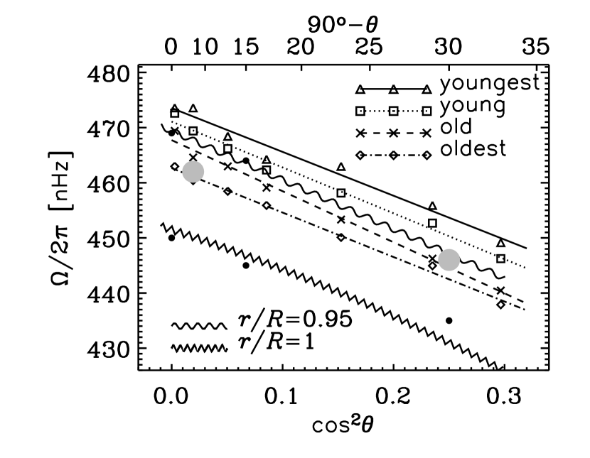
Figure 2.— Angular velocity of sunspots of different age as a function of colatitude $\theta$ compared with the helioseismological internal angular velocity at $r=0.95R$ and with the Doppler velocity at the surface. The large gray dots at about $30^{\circ}$ and $4^{\circ}$ denote the angular velocities of active zones respectively near the beginning and near the end of the cycle. The three small dots near the zig-zag line are the helioseismological angular velocities at $r=0.7R$.

Let us now discuss the properties of a dynamo operating in the bulk or in the upper layers of the sun. We envisage a dynamo that operates very much like a classical $\alpha\Omega$ dynamo as it was proposed in the early days of mean field dynamo theory. In particular, one may anticipate a field that is not strongly fibril, as is indeed confirmed by simulations of turbulent dynamos with shear (Brandenburg, Bigazzi, & Subramanian 2001). Furthermore, in the uppermost $3\,{\rm Mm}$ of the sun turbulent downward transport is far too strong to let any significant field appear at the surface, except in active regions which emerge as the result of strong flux segregation into strongly and weakly magnetized regions, as demonstrated by large aspect ratio magneto-convection simulation (Tao et al. 1998).

There are however several new problems. Most important is the fact that the near surface shear layer is rather thin, so we may have a problem of too many toroidal flux belts if the dynamo was solely confined to the surface layer. There are other possible problems where only a preliminary discussion can be offered. This includes potentially observable effects of near surface magnetic activity on the supergranulation. It is conceivable that the supergranulation may show significant alignment with the mean field. So far, no such anisotropy has been reported, although we do know that the cell size of the normal surface granulation does change with the cycle (Houdek et al. 2001).

The other aspect concerns Joy’s law which has successfully been reproduced within the framework of the thin flux tube approximation. In the context of a distributed dynamo the inclination of bipolar regions is primarily controlled by the sense of the latitudinal shear (patches at higher latitudes lack behind those at lower latitudes). There is also a contribution of $\alpha$ to the tilt (positive $\alpha$ produces positively helical fields whose interceptions with the surface yield a solar tilt). The latter effect is however subdominant, as is seen from a turbulence simulation (see the next section).

We should mention the phenomenon of active zones. They constitute patches of recurrent magnetic activity over months and sometimes years. Recent investigations by Benevolenskaya et al. (1999) showed that these patches have different angular velocity at different depths, corresponding to the local angular velocity at radii between $0.95\,R$ and $0.98\,R$, suggesting again that these magnetic activity complexes are anchored within the near-surface shear layer; see Fig. 1 and the gray dots in Fig. 2. One may picture these activity complexes as more strongly magnetized regions which can only decay slowly, possibly because of magnetic helicity conservation of perhaps because magnetic fields can have a tendency to segregate into strongly and weakly magnetized regions, as is found in large aspect ratio magnetoconvection with imposed field (Tao et al. 1998).

An important consideration for tachocline dynamos is whether the observed emergent flux of $10^{24}\,{\rm Mx}$ over the full solar cycle can be produced (Galloway & Weiss 1981). In the present context we are thinking of mean toroidal fields of the order of $300\,{\rm G}$, which is about one tenth of the strength of the mean field usually envisaged for the overshoot layer. However, because of the larger cross-sectional surface of, say, $(200\,{\rm Mm})^{2}$, this will still produce the required $10^{24}\,{\rm Mx}$.

Global simulations of the solar dynamo are becoming more advanced. The models of Brun et al. (2004) show distributed dynamo action of the type envisaged in this paper. However, these models have some characteristic properties that are different from the observed solar field. Most important is perhaps the relatively large ratio of poloidal to toroidal field, which suggests that the effect of the differential rotation is not sufficiently prominent or, conversely, the effect of the small scale turbulent field is too prominent. In the following we discuss a possible cause of this and address the question how this may change with increasing resolution and larger fluid and magnetic Reynolds numbers.

There are two distinct properties of turbulent dynamo action that seem to depend on microscopic viscosity and diffusivity. First, the magnetic field in the simulations may be dominated by small scale dynamo action (where helicity and shear are unimportant). At small magnetic Prandtl number the small scale dynamo is much harder to excite (Schekochihin et al. 2004a, Boldyrev & Cattaneo 2004, Haugen et al. 2004) and may become subdominant, allowing the large scale dynamo effect to become more prominent. Second, at high magnetic Reynolds numbers the large scale dynamo time scale tends to be constrained by magnetic helicity conservation (Brandenburg 2001). Small scale magnetic helicity fluxes throughout the domain become important to allow – and even facilitate – large scale dynamo action (Blackman & Field 2000, Kleeorin et al. 2000, 2003, Vishniac & Cho 2001, Subramanian & Brandenburg 2004, Brandenburg & Sandin 2004). The convective dynamos in simulations of Brun et al. (2004), for example, generate only a weak mean field. This raises the possibility that such dynamos are of a different type than the large scale dynamo that is believed to operate in the sun. For this reason we now inspect a somewhat different simulation that lacks convection and stratification, but where there is sufficient shear to generate a prominent large scale field. We use this simulation to find some guidance regarding the question of how fibril the field of the sun is and whether it might provide the right conditions for bipolar regions to form.

4. Guidance from simulations

The existence of fibril fields (Parker 1982) is crucial in a scenario where strong flux tubes rise through the convection zone to form sunspot pairs at the surface. The fibril nature of the field is also the main reason why magnetic buoyancy may be so important. Fibril fields have indeed been seen in simulations of forced and convective turbulence where mostly a small scale dynamo is in operation (Nordlund et al. 1992, Politano, Pouquet, & Sulem 1995, Brandenburg et al. 1996). However, this picture changes in the presence of strong shear, for example in the case of accretion disc turbulence (Brandenburg et al. 1995) or in the case of imposed shear (Brandenburg et al. 2001). We begin with a brief description of the model and then discuss whether the field is fibril and whether it is able to form bipolar regions.

4.1. Description of the model

The model discussed in this paper is basically equivalent to the model studied recently by Brandenburg & Sandin (2004), except that no external field is imposed. In this model the turbulence is driven by a forcing function $f$ that consists of eigenfunctions of the curl operator (with wavenumbers $4.5\leq k_{\rm f}\leq 5.5$) and of a large scale component with wavenumber $k_{1}=1$. The domain is of size ${\textstyle{1\over 2}}\pi\times 2\pi\times{\textstyle{1\over 2}}\pi$, representing a cartesian approximation $(x,y,z)$ to a sector in the sun between $0^{\circ}$ and $30^{\circ}$ latitude. Thus, $(x,y,z)$ corresponds to $(r,\phi,-\theta)$, where $\phi$ is longitude and $\theta$ colatitude. The forcing function is arranged such that a mean flow of the form

$$\overline{\bm{U}}=U_{0}\cos k_{1}x\cos k_{1}z,$$ (1)

is driven in the meridional plane $-\pi/2\leq k_{1}x\leq 0$ and $0\leq k_{1}z\leq\pi/2$. In the following we adopt units where $k_{1}=1$. The equator is assumed to be at $z=0$ and the outer surface at $x=0$. The bottom of the convection zone is at $x=-\pi/2$ and $z=\pi/2$ corresponds to the latitude of around $30^{\circ}$, i.e. where the surface angular velocity equals the value in the radiative interior. In the plots below we always display nondimensional combinations by scaling length with $k_{1}$ and time with $u_{\rm rms}k_{1}$.

In this model there is radial shear near the “bottom” of what represents the convection zone and latitudinal shear in the upper parts. At the level of simplification necessary to isolate fundamentally new effects, such as the shear–current effect of Rogachevskii & Kleeorin (2003, 2004) we have refrained from modeling the near-surface shear layer. Furthermore, curvature effects are ignored and no Coriolis force is included, so the $\mbox{\boldmath$\Omega$}{}\times\overline{\bm{J}}$ effect of Rädler (1969) is absent. With nonhelical forcing, the $\overline{\bm{W}}\times\overline{\bm{J}}$ (where $\overline{\bm{W}}=\mbox{\boldmath$\nabla$}{}\times\overline{\bm{U}}$ is the mean vorticity) is however a possible effect driving large scale dynamo action. Nevertheless, we focus on the morphology of the field in the case where the helicity of the forcing is finite and negative – consistent with the conditions in the northern hemisphere of the sun.

We assume an isothermal equation of state with sound speed $c_{\rm s}={\rm const}{}$, and solve the continuity, momentum, and induction equations in the form

$${{\rm D}{}\ln\rho\over{\rm D}{}t}=-\mbox{\boldmath$\nabla$}{}\cdot{\bm{U}},$$ (2)

$${{\rm D}{}{\bm{U}}\over{\rm D}{}t}=-c_{\rm s}^{2}\mbox{\boldmath$\nabla$}{}\ln\rho+{{\bm{J}}\times{\bm{B}}\over\rho}+\mbox{\boldmath$f$}{}+{\bm{F}}_{\rm visc},$$ (3)

$${\partial{\bm{A}}\over\partial t}={\bm{U}}\times{\bm{B}}-\eta\mu_{0}{\bm{J}},$$ (4)

where $\rho$ is density, ${\bm{U}}$ is velocity, ${\bm{J}}=\mbox{\boldmath$\nabla$}{}\times{\bm{B}}/\mu_{0}$ is current density, ${\bm{B}}=\mbox{\boldmath$\nabla$}{}\times{\bm{A}}$ is magnetic field expressed in terms of the magnetic vector potential, $\eta$ is the magnetic diffusivity, and

$${\bm{F}}_{\rm visc}=\nu\left(\nabla^{2}{\bm{U}}+{\textstyle{1\over 3}}\mbox{\boldmath$\nabla$}{}\mbox{\boldmath$\nabla$}{}\cdot{\bm{U}}+2\mbox{\boldmath$\sf S$}{}\cdot\mbox{\boldmath$\nabla$}{}\ln\rho\right)$$ (5)

is the viscous force where $\nu=\mbox{const}$ is the kinematic viscosity, and ${\sf S}_{ij}=\frac{1}{2}(U_{i,j}+U_{j,i})-\frac{1}{3}\delta_{ij}U_{k,k}$ the traceless rate of strain tensor.

We step the equations forward in time by using the Pencil Code, which is a high order finite difference code (sixth order in space and third order in time) for solving the compressible hydromagnetic equations on distributed memory machines using the Message Passing Interface libraries. The numerical resolution is $128\times 512\times 128$ meshpoints. The boundary conditions are periodic in the $y$ direction and stress-free in the $x$ and $z$ directions. For the magnetic field we assume perfect conductor boundary conditions at what corresponds to the base of the convection zone ($k_{1}x=-\pi/2$) and at mid-latitudes ($k_{1}z=\pi/2$). At the equator ($z=0$) and at the outer surface ($x=0$) we assume the magnetic field to be normal to the boundaries, i.e. ${\bm{B}}\times\hat{\mbox{\boldmath$n$}}{}=0$. We refer to these boundaries as “open”, because they permit magnetic and current helicity fluxes, as opposed to “closed” or perfectly conducting boundaries where ${\bm{B}}\cdot\hat{\mbox{\boldmath$n$}}{}=0$ with no helicity fluxes.

The strength of the forcing is chosen such that the typical rms velocity of the turbulence (without the systematic shear flow) is subsonic with $u_{\rm rms}/c_{\rm s}=0.1$. Viscosity and magnetic diffusivity are chosen such that $\nu/\eta=1$ and $R_{\rm m}=u_{\rm rms}/(\eta k_{\rm f})\approx 80$. In the simulations with negative helical forcing, the turbulent part of the velocity field is nearly fully helical, i.e. $\langle\mbox{\boldmath$\omega$}{}\cdot{\bm{u}}\rangle/(k_{\rm f}u_{\rm rms}^{2})\approx-1$. The mean flow is about 5 times stronger than the turbulent flow, i.e. $U_{0}/u_{\rm rms}\approx 5$.

4.2. Growth of the large scale field

A series of experiments has been performed: with helical forcing of negative helicity (representative of the northern hemisphere; denoted by “$\alpha>0$” since the resulting electromotive force would lead to a positive $\alpha$ effect), positive helicity (mainly for comparison, but it could be representative of the bottom of the convection zone; denoted by “$\alpha<0$”), and without helicity (denoted by “$\alpha=0$”). In all cases the kinematic growth rate is about the same (${\rm d}{}\ln B_{\rm rms}/{\rm d}{}t=0.02\,u_{\rm rms}k_{\rm f}$).

Figure 3.— Evolution of the energies of the total field $\langle{\bm{B}}^{2}\rangle$ and of the mean field $\langle\overline{\bm{B}}^{2}\rangle$, in units of $B_{\rm eq}^{2}$, for runs with non-helical forcing and open or closed boundaries; see the solid and dotted lines, respectively. The inset shows a comparison of the ratio $\langle\overline{\bm{B}}^{2}\rangle/\langle{\bm{B}}^{2}\rangle$ for nonhelical ($\alpha=0$) and helical ($\alpha>0$) runs. For the nonhelical case the run with closed boundaries is also shown (dotted line near $\langle\overline{\bm{B}}^{2}\rangle/\langle{\bm{B}}^{2}\rangle\approx 0.07$). Note that saturation of the large scale field occurs on a dynamical time scale; the resistive time scale is given on the upper abscissa.

In Brandenburg & Sandin (2004) the effect of boundaries was already found to be important: when a perfect conductor condition was used at the equator and at the outer surface the resulting $\alpha$ effect was found to be suppressed by a factor of $\sim 30$. In the present case we find that near saturation the large scale field remains well below equipartition (see the dotted line in Fig. 3). With open boundary conditions, near-equipartition field strengths can be achieved ($\overline{\bm{B}}^{2}/B_{\rm eq}^{2}\approx 0.8$). Here we define $\overline{\bm{B}}$ as an average over the $y$ direction (toroidal average). Volume averages are denoted by angular brackets.

In the presence of finite helicity the result is not greatly affected; see the inset of Fig. 3 where we show that the ratio $\langle\overline{\bm{B}}^{2}\rangle/\langle{\bm{B}}^{2}\rangle$ either varies around 0.5 (for $\alpha>0$ or $\alpha<0$), or that it stays around 0.7 (for $\alpha=0$). The case $\alpha<0$ is not shown here, but we refer to Brandenburg et al. (2005) for a description of those results.

So far we have not seen reversals of the field. We note, however, that in principle cycles are possible in this type of geometry and have indeed be found both in the corresponding mean field model (Brandenburg & Sandin 2004). In the present case the lack of cycles could be connected with the resulting mean flow that was neglected in the mean field calculations. [On the average, however, the mean poloidal flow (poleward at the surface) is less than 2% of the total mean flow. By comparison, the mean poloidal field is about 25% of the total mean field; see §4.4.]

Our main conclusion from these simulations is that large scale dynamo action can produce equipartition field strengths on a dynamical time scale, provided the boundaries are open. The significance of open boundaries is that magnetic and current helicity can leave the domain, thus preventing the excessive build-up of small scale magnetic helicity before the large scale field has saturated.

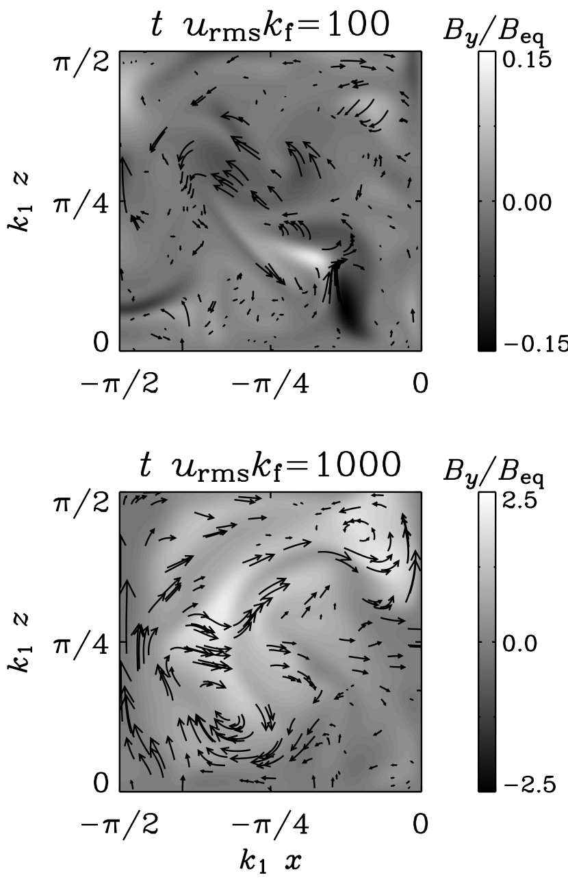
Figure 4.— Snapshots of the magnetic field ${\bm{B}}$ in the meridional plane during the kinematic stage ($t=100$ turnover times) and the saturated stage ($t=1000$ turnover times). Vectors in the meridional plane are superimposed on a gray scale representation of the azimuthal field. The gray scale is symmetric about mid-gray shades, so the absence of dark shades (e.g. in the lower panel) indicates the absence of negative values. Note the development of larger scale structures during the saturated stage with basically unidirectional toroidal field.

4.3. How fibril is the field?

Virtually all dynamo simulations (both small scale and large scale) show that once the dynamo saturates, the typical length scale of the field increases, as measured for example by the magnetic Taylor microscale $\lambda_{\rm M}$, where $\lambda_{\rm M}^{2}=5\mu_{0}^{2}\langle{\bm{J}}^{2}\rangle/\langle{\bm{B}}^{2}\rangle$; see Schekochihin et al. (2004b) for the case of a forced small scale dynamo and Brandenburg et al. (1996) for the case of a small scale dynamo in convective turbulence. In practice this means that the typical scale of the flux structures increases during the saturation. However, the orientation of the field is otherwise still random. The presence of shear together with turbulent diffusion has a strong tendency to order the field such that it points everywhere in the same direction. This tendency has been studied earlier in connection with a completely random (incoherent) $\alpha$ effect (Vishniac & Brandenburg 1997). This tendency is seen in the present simulations as well; see Fig. 4, where we show meridional cross-sections of the field during kinematic and saturated phases. From the simulations presented here we cannot support the assumption that in the solar convection zone the field will be highly fibril.

Compared to the sun, there is of course the difference that the turbulence is not driven by a body force, but by convection. However, it is not clear that this will make an important difference. It is also possible that at larger magnetic Reynolds numbers there will be a stronger tendency to produce intense fibrils. However, for the present simulations with $128\times 512\times 128$ meshpoints the viscosity is already as small as possible. In fact, the magnetic Reynolds number based on the mesh spacing, $\delta x$, of $R_{\rm m}k_{\rm f}\delta x\approx 5$, which is a typical value that should not be exceeded in these type of simulations.

Once we abandon the rising flux tube picture, we have to think of other ways to produce bipolar regions with the right tilt angle. This will be discussed in the next section.

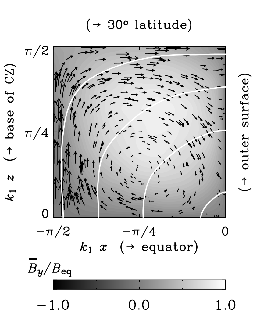
Figure 5.— Gray scale representation of the azimuthally and time averaged mean azimuthal field $\overline{\bm{B}}(x,z)$ together with vectors in the meridional plane. The mean toroidal velocity is shown as white contours. The projected positions on the sun are labeled on the corresponding axes. Note the equatorward orientation of the poloidal field near the outer surface ($x=0$). As in Fig. 4, the gray scale is symmetric about mid-gray shades, so the absence of dark shades indicates that $\overline{B}_{y}>0$. In this run the kinetic helicity is negative, corresponding to $\alpha>0$. The root mean square of the mean poloidal field is $\sim 25\%$ of the total mean field.

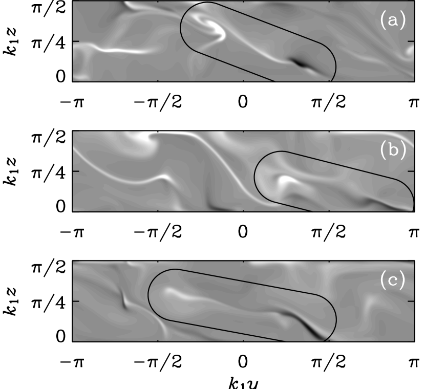
Figure 6.— Magnetograms of the radial field $B_{x}(y,z,t)$ at the outer surface ($x=0$) on the northern hemisphere at times $t/\tau=480$, $750$, and $990$, where $\tau=(u_{\rm rms}k_{\rm f})^{-1}$ is the turnover time, and $k_{\rm f}$ is the wavenumber corresponding to the energy-carrying scale of the turbulence. Light shades correspond to field vectors pointing out of the domain, and dark shades correspond to vectors pointing into the domain. The elongated rings highlight the positions of bipolar regions. Note the clockwise tilt relative to the $y$ (or toroidal) direction, and the systematic sequence of polarities (white left and dark right) corresponding to $\overline{B}_{y}>0$, which is consistent with Fig. 5.

4.4. Formation of bipolar regions

In the present simulations, because of shear, most of the field is in the streamwise direction. On the open boundaries, on the other hand, the field can only be normal to the boundary and hence $B_{y}=0$. However, because elsewhere in the interior, the field is mostly toroidal, places with significant normal field (${\bm{B}}\cdot\hat{\mbox{\boldmath$n$}}{}\neq 0$) will be rare. This is also what is seen in the simulations; see Fig. 6, were we show “magnetograms” of the normal field on the outer surface, $x=0$. A meridional cross-section of the azimuthally and temporally averaged field, $\overline{\bm{B}}$, is shown in Fig. 5. Here the identification with a sector in a meridional plane of the sun is annotated on the axes. Except near the open boundaries, where $\overline{B}_{y}=0$, the mean field is mostly into the plane ($\overline{B}_{y}>0$) and is accompanied by a right-handed swirl so that $\overline{B}_{z}<0$ on the outer surface, $x=0$.

What the magnetograms in Fig. 6 show is basically a gray background (corresponding to zero field) with only a few patches, some of which come in pairs. Often the pairs are connected by a faint “bridge”. In all cases the bipolar regions as well as the bridges are inclined relative to the toroidal direction by an inclination angle that is primarily determined by the latitudinal shear. Any cross-stream (i.e. latitudinally oriented) field becomes sheared out and intensifies until the structure disappears. The polarity depends on the sign of the latitudinal ($z$) component of the field beneath the surface. The phases of maximum intensity correspond to times when structures are most prominent; see Fig. 6. Control simulations with opposite sign of helicity confirm that the inclination is qualitatively unchanged and that the poloidal field determines the orientation of the polarities, not the toroidal field. If the tilt was entirely determined by the negative $\alpha$, it would have produced tilt in the opposite sense. In the present case of negative kinetic helicity in the northern hemisphere ($\alpha>0$), as in the upper parts of the solar convection zone, the $\alpha$ effect would produce tilt of the same sign as the shear. However, as we have seen above, the effect of $\alpha$ on the tilt is subdominant in the present simulations, where the effect of shear is strong.

The typical separation of the different polarities corresponds to about 1–2 eddy scales ($=2\pi/k_{\rm f}$). Comparing to the sun, the pressure scale height at $r=0.95R$ is $12\,{\rm Mm}$, so the mixing length and hence the eddy scale is $\sim 20\,{\rm Mm}$. Thus, the typical size of the active region in the model is $\sim 30\,{\rm Mm}$.

We conclude from this section that the tilt of bipolar regions depends mainly on the latitudinal differential rotation, and that the orientation of the polarities depends on the orientation of the latitudinal component of the field rather than its azimuthal component. The sense of the tilt is thus independent of the sign of $\alpha$. The simulations suggest that more or less isolated bipolar regions can emerge in a way that is at least as plausible as the picture of strong tilted flux tube poking through the surface from deep underneath.

5. Conclusions

It has long been known that sunspots and other magnetic tracers rotate faster than the photospheric plasma. Originally, this was taken as evidence that the sun must rotate faster in the interior (Golub et al. 1981). In fact, it was believed that the angular velocity of sunspots agrees with the local angular velocity at the depth where the sunspots are anchored. Since the mid-eighties this idea became largely discarded on the grounds that helioseismology began to show angular velocity contours that are nearly spoke-like and that the only location of radial shear was the bottom of the convection zone. From a dynamo theorist’s point of view this result, together with the already popular idea that the solar dynamo should operate at or below the bottom of the convection zone (Table 1), meant that at least the issue of the location of the dynamo had been settled. This picture was in principle quite appealing and it became particularly attractive in combination with the subsequent finding that the right tilt angles can be obtained when the fields at the bottom of the convection zone are of the order of $10^{5}\,{\rm G}$ (D’Silva & Choudhuri 1993).

Two important results have emerged since then. First, downward pumping tends to be a strong effect that can overcome magnetic buoyancy up to fairly large field strengths. Second, helioseismology has now revealed the presence of a near-surface shear layer that is stronger and more prominent than indicated by the early results of helioseismology. In the tachocline, by comparison, the radial shear layer is rather weak at $30^{\circ}$ latitude (which is where sunspots emerge in the beginning of the cycle) and extremely strong at the poles (where the magnetic activity is weak). It appears that the impact of these findings on the solar dynamo paradigm ought to be reconsidered. The purpose of the present paper was therefore to present the arguments for and against tachocline dynamos versus distributed dynamos that are possibly strongly affected or shaped by the near-surface shear layer. The reason we use word “shaped” is to indicate that the dynamo is likely to operate in the entire convection zone, and not only in the near-surface shear layer.

The idea that sunspots might be anchored at a depth of 0.95 solar radii has however a problem. The helioseismologically determined angular velocity at that depth is still $\sim 4\,{\rm nHz}$ slower than that of the very youngest sunspots. This corresponds to a velocity difference of $\sim 20\,{\rm m/s}$. In principle, if the profile of such enhanced angular velocity is sufficiently localized, one might argue that the spatial resolution of helioseismology was still insufficient. Alternatively, and perhaps more likely, there may still be some not yet understood mechanism causing newly emerging flux to rotate slightly faster.

An important part of the flux tube paradigm is the idea that strong flux tubes emerge from deep underneath and form bipolar regions and sunspot pairs as they reach the surface. This picture relies entirely on the thin flux tube approximation, which may have its own difficulties (Dorch & Nordlund 1998, Wissink et al. 2000). However, as demonstrated in §4 and through Fig. 6, a distributed dynamo is quite able to produce bipolar regions with plausible tilt angles. As discussed at the end of §4.4, the orientation of the tilt is controlled by the latitudinal shear. The orientation of the polarities is determined by the direction of the poloidal field, and not the azimuthal field.

Since this model lacks convection and stratification, both turbulence and shear have to be produced by body forces. Nevertheless, the model is fully self-consistent and not subject to approximations, such as the thin flux tube approximation. Obviously, an important next step should be to include convection and stratification. Equally important is the implementation of a more realistic outer boundary condition, possibly allowing for the development of coronal mass ejections that might be necessary for carrying small scale magnetic and current helicities away from the dynamo. Proper modeling of coronal mass ejections might require the use of spherical geometry. A lack of magnetic and current helicity fluxes out of the domain would prevent the dynamo from operating on a dynamical time scale (Blackman & Field 2000). On the other hand, some degree of throttling of the helicity flux might actually occur in the sun. This might explain why the solar cycle period tends to be about 10 times longer than what is suggested by standard mean field models (Köhler 1973) using canonical estimates for the turbulent diffusivity (Krivodubskii 1984). Obviously, a reasonably accurate theory of helicity fluxes is required before this question can be addressed in mean field calculations.

$Header: /home/brandenb/CVS/tex/mhd/surfdiffrot/ms.tex,v 1.95 2005/02/15 20:30:21 brandenb Exp $

References

- (1) Balthasar, H., Schüssler, M., & Wöhl, H. 1982, Solar Phys., 76, 21
- (2) Basu, S. 1997, MNRAS, 288, 572
- (3) Baumann, I., Schmitt, D., Schüssler, M., & Solanki, S. K. 2004, A&A, 426, 1075
- (4) Benevolenskaya, E. E., Hoeksema, J. T., Kosovichev, A. G., & Scherrer, P. H. 1999, ApJ, 517, L163
- (5) Blackman, E. G., & Field, G. F. 2000, ApJ, 534, 984
- (6) Boldyrev, S., & Cattaneo, F. 2004, PRL, 92, 144501
- (7) Brandenburg, A. 2001, ApJ, 550, 824
- (8) Brandenburg, A., & Sandin, C. 2004, A&A, 427, 13
- (9) Brandenburg, A., Bigazzi, A., & Subramanian, K. 2001, MNRAS, 325, 685
- (10) Brandenburg, A., Nordlund, Å., Stein, R. F., & Torkelsson, U. 1995, ApJ, 446, 741
- (11) Brandenburg, A., Jennings, R. L., Nordlund, Å., et al. 1996, JFM, 306, 325
- (12) Brandenburg, A., Haugen, N. E. L., Käpylä, P. J., & Sandin, C. 2005, AN, 326, 174 [arXiv:astro-ph/0412364]
- (13) Brun, A. S., Miesch, M. S. & Toomre, J. 2004, ApJ, 614, 1073
- (14) Busse, F. H. 2004, Chaos, 14, 803
- (15) Caligari, P., Moreno-Insertis, F., & Schüssler, M. 1995, ApJ, 441, 886
- (16) Cattaneo, F. 1999, ApJ, 515, L39
- (17) Chatterjee, P., Nandy, D., & Choudhuri, A. R. 2004, A&A, 427, 1019
- (18) Chou, D.-Y., & Fisher, G. H. 1989, ApJ, 341, 533
- (19) Choudhuri, A. R. 1990, ApJ, 355, 733
- (20) Choudhuri, A. R., Schüssler, M., & Dikpati, M. 1995, A&A, 303, L29
- (21) Corbard, T., & Thompson, M. J. 2001, Solar Phys., 205, 211
- (22) Covas, E., Tavakol, R., Vorontsov, S., & Moss, D. 2001, A&A, 375, 260
- (23) Dorch, S. B. F. & Nordlund, Å. 1998, A&A, 338, 329
- (24) Dorch, S. B. F. & Nordlund, Å. 2001, A&A, 365, 562
- (25) Dikpati, M., & Charbonneau, P. 1999, ApJ, 518, 508
- (26) Dikpati, M., Corbard, T., Thompson, M. J., & Gilman, P. A. 2002, ApJ, 575, L41
- (27) D‘Silva, S., & Choudhuri, A. R. 1993, A&A, 272, 621
- (28) Durney, B. R. 1995, Solar Phys., 166, 231
- (29) Durney, B. R., De Young, D. S., & Roxburgh, I. W. 1993, Solar Phys., 145, 207
- (30) Fan, Y., Zweibel, E. G., Linton, M. G., & Fisher, G. H. 1999, ApJ, 521, 460
- (31) Fan, Y. 2004, Living Rev. Solar Phys., 1, 1, http://www.livingreviews.org/lrsp-2004-1
- (32) Fisher, G. H., Fan, Y., Longcope, D. W., Linton, M. G., & Pevtsov, A. A. 2000, Solar Phys., 192, 119
- (33) Galloway, D., & Weiss, N. O. 1981, Geophys. Astrophys. Fluid Dyn., 243, 945
- (34) Gilman, P. A., & Foukal, P. V. 1979, ApJ, 229, 1179
- (35) Gizon, L., Duvall Jr, T. L., & Schou, J. 2003, Nat, 421, 43
- (36) Golub, L., Rosner, R., Vaiana, G. S., & Weiss, N. O. 1981, ApJ, 243, 309
- (37) Haugen, N. E. L., Brandenburg, A., & Dobler, W. 2004, PRE, 70, 016308
- (38) Houdek, G., Chaplin, W. J., Appourchaux, T., et al. 2001, MNRAS, 327, 483
- (39) Howard, R., & LaBonte, B. J. 1980, ApJ, 239, L33
- (40) Howe, R., Christensen-Dalsgaard, J., Hill, F., et al. 2000a, Sci, 287, 2456
- (41) Howe, R., Christensen-Dalsgaard, J., Hill, F., et al. 2000b, ApJ, 533, L163
- (42) Kazantsev, A. P. 1968, Sov. Phys. JETP, 26, 1031
- (43) Kitchatinov, L. L., & Mazur, M. V. 2000, Solar Phys., 191, 325
- (44) Kleeorin, N. I., Mond, M., & Rogachevskii, I. 1996, A&A, 307, 293
- (45) Kleeorin, N. I, Moss, D., Rogachevskii, I., & Sokoloff, D. 2000, A&A, 361, L5
- (46) Kleeorin, N. I., Kuzanyan, K., Moss, D., et al. 2003, A&A, 409, 1097
- (47) Köhler, H. 1973, A&A, 25, 467
- (48) Kosovichev, A. G., Duvall, T. L. Jr., & Scherrer, P. H. 2000, Solar Phys., 192, 159
- (49) Kosovichev, A. G. 2002, AN, 323, 186
- (50) Krivodubskii, V. N. 1984, Sov. Astron., 28, 205
- (51) Küker, M., Rüdiger, G., & Schultz, M. 2001, A&A, 374, 301
- (52) Linton, M. G., Longcope, D. W., & Fisher, G. H. 1996, ApJ, 469, 954
- (53) Markiel, J. A., & Thomas, J. H. 1999, ApJ, 523, 827
- (54) Mason, J., Hughes, D. W., & Tobias, S. M. 2002, ApJ, 580, L89
- (55) Miesch, M. S., Elliott, J. R., Toomre, J., et al. 2000, ApJ, 532, 593
- (56) Moreno-Insertis, F. 1986, A&A, 166, 291
- (57) Moreno-Insertis, F., & Emonet, T. 1996, ApJ, 472, L53
- (58) Moreno-Insertis, F., Schüssler, M., & Ferriz-Mas, A. 1992, A&A, 264, 686
- (59) Moreno-Insertis, F., Caligari, P., & Schüssler, M. 1995, ApJ, 452, 894
- (60) Moss, D., Tuominen, I., & Brandenburg, A. 1990, A&A, 240, 142
- (61) Nandy, D., & Choudhuri, A. R. 2002, Sci, 296, 1671
- (62) Nesme-Ribes, E., Ferreira, E. N., & Mein, P. 1993, A&A, 274, 563
- (63) Nordlund, Å., Brandenburg, A., Jennings, et al. 1992, ApJ, 392, 647
- (64) Ossendrijver, M. 2003, A&AR, 11, 287
- (65) Ossendrijver, M., Stix, M., Brandenburg, A., & Rüdiger, G. 2002, A&A, 394, 735
- (66) Parker, E. N. 1975, ApJ, 198, 205
- (67) Parker, E. N. 1979, Cosmical Magnetic Fields (Clarendon Press, Oxford)
- (68) Parker, E. N. 1982, ApJ, 256, 302
- (69) Parker, E. N. 1993, ApJ, 408, 707
- (70) Politano, H., Pouquet, A., & Sulem, P. L. 1995, Phys. Plasmas, 8, 2931
- (71) Pulkkinen, P., & Tuominen, I. 1998, A&A, 332, 748
- (72) Rädler, K.-H. 1969, Geod. Geophys. Veröff., Reihe II, 13, 131
- (73) Rempel, M., & Schüssler, M. 2001, ApJ, 552, L171
- (74) Rogachevskii, I., & Kleeorin, N. 2003, PRE, 68, 036301
- (75) Rogachevskii, I., & Kleeorin, N. 2004, PRE, 70, 046310
- (76) Rüdiger, G., & Brandenburg, A. 1995, A&A, 296, 557
- (77) Rüdiger, G., & Kitchatinov, L. L. 1993, A&A, 269, 581
- (78) Schekochihin, A. A., Cowley, S. C., Maron, J. L., McWilliams, J. C. 2004a, PRL, 92, 054502
- (79) Schekochihin, A. A., Cowley, S. C., Taylor, S. F., et al. 2004b, ApJ, 612, 276
- (80) Schrijver, C. J., & Title, A. M. 1999, Solar Phys., 188, 331
- (81) Schou, J. 2003, ApJ, 596, L259
- (82) Schüssler, M. 1983, in Solar and stellar magnetic fields: origins and coronal effects, ed. J. O. Stenflo (Reidel), 213
- (83) Schüssler, M. 1984, in The Hydromagnetics of the Sun, ed. T. D. Guyenne & J. J. Hunt (ESA SP-220), 67
- (84) Schüssler, M. 2002, AN, 323, 377
- (85) Schüssler, M. 2005, AN, (in press)
- (86) Schüssler, M., Caligari, P., Ferriz-Mas, A., & Moreno-Insertis, F. 1994, A&A, 281, L69
- (87) Spiegel, E. A., & Weiss, N. O. 1980, Nat, 287, 616
- (88) Spiegel, E. A., & Zahn, J.-P. 1992, A&A, 265, 106
- (89) Spruit, H. C. 1974, Solar Phys., 34, 277
- (90) Spruit, H. C. 1981, A&A, 102, 129
- (91) Spruit, H. C., & Zweibel, E. G. 1979, Solar Phys., 62, 15
- (92) Stix, M. 1974, A&A, 37, 121
- (93) Stix, M. 1976, A&A, 47, 243
- (94) Subramanian, K., & Brandenburg, A. 2004, PRL, 93, 205001
- (95) Tao, L., Weiss, N. O., Brownjohn, D. P., & Proctor, M. R. E. 1998, ApJ, 496, L39
- (96) Tobias, S. M., Brummell, N. H., Clune, T. L., & Toomre, J. 1998, ApJ, 502, L177
- (97) Tobias, S. M., Brummell, N. H., Clune, T. L., & Toomre, J. 2001, ApJ, 549, 1183
- (98) Tobias, S. M. 2002, Phil. Trans. Roy. Soc., A 360, 2741
- (99) Thomas, J. H., Weiss, N. O., Tobias, S. M., & Brummell, N. H. 2002, Nat, 420, 390
- (100) Thompson, M. J., Christensen-Dalsgaard, J., Miesch, M. S., & Toomre, J. 2003, ARA&A, 41, 599
- (101) Tuominen, J. 1962, Z. f. Ap., 55, 110
- (102) Tuominen, I., & Virtanen, H. 1988, Adv. Space Sci., 8, 141
- (103) van Ballegooijen, A. A. 1982, A&A, 113, 99
- (104) Vilhu, O. 1984, A&A, 133, 117
- (105) Vishniac, E. T., & Brandenburg, A. 1997, ApJ, 475, 263
- (106) Vishniac, E. T., & Cho, J. 2001, ApJ, 550, 752
- (107) Vorontsov, S. V., Christensen-Dalsgaard, J., Schou, J., et al. 2002, Sci, 296, 101
- (108) Weiss, N. O., Thomas, J. H., Brummell, N. H., & Tobias, S. M. 2004, ApJ, 600, 1073
- (109) Weiss, N. O. 2005, AN, (in press)
- (110) Wilson, P. R. 1987, Solar Phys., 110, 59
- (111) Wissink, J. G., Matthews, P. C., Hughes, D. W., & Proctor, M. R. E. 2000, ApJ, 536, 982
- (112) Yoshimura, H. 1972, ApJ, 178, 863
- (113) Yoshimura, H. 1976, Solar Phys., 50, 3
- (114) Ziegler, U., & Rüdiger, G. 2003, A&A, 401, 433
- (115) Zwaan, C. 1978, Solar Phys., 60, 213