Testing Stellar Models With An Improved Physical Orbit for 12 Boötis

Abstract

In a previous publication we reported on the binary system 12 Boötis and its evolutionary state. In particular the 12 Boo primary component is in a rapid phase of evolution, hence accurate measurement of its physical parameters makes it an interesting test case for stellar evolution models. Here we report on a significantly improved determination of the physical orbit of the double-lined spectroscopic binary system 12 Boo. We have a 12 Boo interferometry dataset spanning six years with the Palomar Testbed Interferometer, a smaller amount of data from the Navy Prototype Optical Interferometer, and a radial velocity dataset spanning 14 years from the Harvard-Smithsonian Center for Astrophysics. We have updated the 12 Boo physical orbit model with our expanded interferometric and radial velocity datasets. The revised orbit is in good agreement with previous results, and the physical parameters implied by a combined fit to our visibility and radial velocity data result in precise component masses and luminosities. In particular, the orbital parallax of the system is determined to be 27.74 $\pm$ 0.15 mas, and masses of the two components are determined to be 1.4160 $\pm$ 0.0049 M_☉ and 1.3740 $\pm$ 0.0045 M_☉, respectively. These mass determinations are more precise than the previous report by a factor of four to five.

As indicated in the previous publication, even though the two components are nearly equal in mass, the system exhibits a significant brightness difference between the components in the near infrared and visible. We attribute this brightness difference to evolutionary differences between the two components in their transition between main sequence and giant evolutionary phases, and based on theoretical models we can estimate a system age of approximately 3.2 Gyr. Comparisons with stellar models suggest that the 12 Boo primary may be just entering the Hertzsprung gap, but that conclusion is highly dependent on details of the models. Such a dynamic evolutionary state makes the 12 Boo system a unique and important test for stellar models.

1 Introduction

12 Boötis (d Boötes, HR 5304, HD 123999, HIP 69226) is a short-period (9.6 d) binary system with nearly-equal mass ($q\sim$ 0.97) components. The system was first detected as a radial velocity variable over 100 years ago (Campbell & Wright, 1900), and the first “good” double-lined orbit was calculated by Abt & Levy (1976). The Abt & Levy (1976) orbit has been reconfirmed by an independent CORAVEL radial velocity orbit by De Medeiros & Udry (1999, hereafter DU99) (data from which was used in Boden et al., 2000). The composite system has been consistently assigned the spectral type F8IV – F9IVw, the latter by Barry (1970), with the “w” indicating weak ultraviolet metallic features. All studies seem to confirm that 12 Boo (catalog HD 123999) has heavy element abundances near solar proportions (Duncan, 1981; Balachandran, 1990; Lèbre et al., 1999; Nordström et al., 2004).

Previously we reported a physical orbit model for the 12 Boo system (Boden et al., 2000, hereafter Paper 1). Paper 1 discussed the interesting evolutionary state of the 12 Boo components; despite the nearly equal mass ratio, the 12 Boo components exhibit an unusual intensity ratio due to their positions on the Hertzsprung-Russel diagram. However, the orbit model of Paper 1 relied upon rather limited radial velocity data. Given this shortcoming and the favorable geometry of the 12 Boo system for high-precision study, we decided to refine the orbit model in order to fully exploit the 12 Boo components as a test of stellar models. Consequently, herein we report on a significantly improved determination of the 12 Boo physical orbit from an expanded set of near-infrared, long-baseline interferometric measurements taken with the Palomar Testbed Interferometer (PTI) and Navy Prototype Optical Interferometer (NPOI), and a large set of new spectroscopic radial velocity measurements obtained at the Harvard-Smithsonian Center for Astrophysics (CfA).

In the following we discuss the new observations (§2), the orbit model (§3) and physical properties (§4) derived from them, and compare the component properties with stellar models (§5). We summarize our findings in §6.

2 Observations

Interferometry

As in Paper 1, the interferometric observable used for these measurements is the fringe contrast or visibility (squared) of an observed brightness distribution on the sky. PTI was used to make the interferometric measurements presented here; PTI is a long-baseline $H$ (1.6$\mu$m) and $K$-band (2.2$\mu$m) interferometer located at Palomar Observatory, and described in detail elsewhere (Colavita et al., 1999). The analysis of such data in the context of a binary system is discussed in detail in Paper 1 and elsewhere (e.g. Hummel et al., 2001) and will not be repeated here.

12 Boo was observed in conjunction with objects in our calibrator list by PTI in $K$ band ($\lambda\sim 2.2\mu$m) on 67 nights between 21 June 1998 and 18 June 2004, a dataset covering roughly six years and 228 orbital periods. Additionally, 12 Boo was observed by PTI in $H$ band ($\lambda\sim 1.6\mu$m) on 12 nights between 28 May 1999 and 15 June 2001. 12 Boo, along with calibration objects, was usually observed multiple times during each of these nights, and each observation, or scan, was approximately 130 sec long. For each scan we computed a mean $V^{2}$ value from the scan data, and the error in the $V^{2}$ estimate from the rms internal scatter (Colavita, 1999). 12 Boo was always observed in combination with one or more calibration sources within $\sim$ 10^∘ on the sky. As in Paper 1, here we have used three stars as calibration objects: HD 121107 (catalog HD 121107) (G5 III), HD 128167 (catalog HD 128167) (F2 V), and HD 123612 (catalog HD 123612) (K5 III). Table 1 lists the relevant physical parameters for the calibration objects.

Table 1: PTI 12 Boo $V^{2}$ Calibration Objects Considered in our Analysis. The relevant parameters for our three calibration objects are summarized. Apparent diameter values are determined from spectral energy distribution modeling of archival broad-band photometry and spectral typing, and visibility measurements with PTI.

Object	Spectral	Star	Separation	Adopted Model
Name	Type	Magnitude	from 12 Boo	Diameter (mas)
HD 121107	G5 III	5.7 $V$/4.0 $K$	8.2∘	0.83 $\pm$ 0.06
HD 128167	F2 V	4.5 $V$/3.5 $K$	7.1∘	0.77 $\pm$ 0.04
HD 123612	K5 III	6.6 $V$/3.1 $K$	0.92∘	1.29 $\pm$ 0.10

The calibration of 12 Boo $V^{2}$ data is performed by estimating the interferometer system visibility ($V^{2}_{sys}$) using calibration sources with model angular diameters, and then normalizing the raw 12 Boo visibility by $V^{2}_{sys}$ to estimate the $V^{2}$ measured by an ideal interferometer at that epoch (Mozurkewich et al., 1991; Boden et al., 1998). Calibrating our 12 Boo dataset with respect to the three calibration objects listed in Table 1 results in a total of 303 calibrated scans (258 in $K$, 46 in $H$) on 12 Boo over 78 nights, roughly quadrupling the visibility dataset from Paper 1. Our calibrated synthetic wide-band $V^{2}$ measurements are summarized in Table 2. In particular, all $V^{2}$ data from Paper 1 are also contained in Table 2 and used in this analysis. Table 2 gives $V^{2}$ measurements and times, measurement errors, residuals between our data and orbit model (Table 4) predictions, the photon-weighted average wavelength, $u-v$ coordinates, and on-target hour angle for each of our calibrated PTI 12 Boo $V^{2}$ observations.

In addition to the PTI visibility data, we have obtained new visibility and closure-phase data on 12 Boo with the Navy Prototype Optical Interferometer (NPOI; Armstrong et al., 1998; Hummel et al., 2003). NPOI observed 12 Boo and calibrator HD 128167 (Table 1) on 13 nights from 9 April 2001 through 28 June 2001 inclusive. On five nights, the NPOI C, E, and W stations were used with maximum baseline of 38 m, and on all other nights the W7, E, and W stations with a maximum baseline of 64 m. The data were taken in 10 narrow-band channels spanning a passband between 650 nm and 850 nm. Unlike the single-baseline PTI $V^{2}$ data, NPOI data were all taken simultaneously using three NPOI baselines; in addition to visibility amplitude such data provide phase-closure information. In particular the NPOI phase-closure data breaks the $\Omega$/inversion degeneracy inherent in the PTI $V^{2}$ (see § 3). The NPOI data were reduced and calibrated according to the standard procedures outlined by Hummel et al. (1998).

Spectroscopy

The largest shortcoming in the orbit model from Paper 1 was the limited and inhomogeneous radial velocity (RV) data. To improve this situation we have obtained 49 new high-resolution spectra of the 12 Boo system at CfA, with an échelle spectrograph mounted at the Cassegrain focus of the 1.5-m Wyeth reflector at the Oak Ridge Observatory (Harvard, Massachusetts). The resolving power of this instrument is $\lambda/\Delta\lambda\approx 35,000$. A single échelle order spanning 45 Å was recorded with a photon-counting Reticon detector, at a central wavelength of 5188.5 Å, near the Mg I b triplet. 12 Boo observations were carried out between June 1987 and April 2001, spanning nearly 14 years and 526 system periods.

Component velocities were determined from the spectra using the TODCOR two-dimensional cross-correlation technique (Zucker & Mazeh, 1994), with synthetic templates for the each star based on Kurucz model atmospheres (available at http://cfaku5.cfa.harvard.edu). The optimal parameters for the templates (mainly effective temperature and rotational velocity) were determined by seeking the best match to the observed spectra as judged from the peak cross-correlation value averaged over all exposures. We obtained $v\sin i$ values of 14  km s^-1 and 12  km s^-1 for the primary (more massive star) and secondary, respectively, with estimated errors of 1  km s^-1. The effective temperatures are sensitive to the adopted surface gravity and chemical composition. For estimated $\log g$ values of 3.8 and 4.0 (see § 4), we obtained by interpolation temperatures of 6130 K and 6230 K for the primary and secondary with adopted uncertainties of 100 K and 150 K, respectively. These are in good agreement with photometric estimates for 12 Boo (§4). Tests with adopted metallicities between [m/H]$=-1.0$ and [m/H]$=+0.5$ in steps of 0.5 dex indicated a preference for solar composition, consistent with recent estimates from the literature. We also determined the light ratio from our spectra following Zucker & Mazeh (1994). The result is $L_{\rm sec}/L_{\rm prim}=0.64\pm 0.02$ at the mean wavelength of our observations, which is close to the visual band.

The radial velocities were tested for systematics by performing numerical simulations following Torres et al. (2002), and small adjustments (typically less than 0.5  km s^-1) were applied to the raw velocities as corrections. The stability of the zero point of our velocity system was monitored by means of exposures of the dusk and dawn sky, and small systematic run-to-run corrections were applied in the manner described by Latham (1992). The final radial velocities are given in Table 2, which gives measured primary and secondary velocities and associated uncertainties, residuals between the measurements and predictions from our orbit model (Table 4), and model phase.

3 Orbit Model

As in previous papers in this series (Boden et al., 1999a, b, 2000; Boden & Lane, 2001; Torres et al., 2002), the estimation of the 12 Boo orbit is made by fitting a Keplerian orbit model directly to the calibrated PTI $V^{2}$ and RV data on 12 Boo (see also Armstrong et al., 1992; Hummel et al., 1993, 1995, 1998, 2001). As discussed in these references, the nature of $V^{2}$ data require that orbital parameter estimation necessarily include in-band component intensity ratios and component diameters (diameters here were held fixed at photometrically estimated values; see §4). Given the well-established 12 Boo model from Paper 1, the additional data presented here are straightforwardly used to refine the previous orbit model.

In general the NPOI data were found to agree well with the orbit estimated from the PTI $V^{2}$ and RV data. However with the exception of the closure phases these data did little to further constrain the orbit parameters. Therefore we have adopted the general orbit orientation (i.e. $\Omega$) indicated by the NPOI closure phases, but the high-precision orbital parameters are derived solely from the PTI $V^{2}$ (Table 2) and RV (Table 2) data.

Figure 1 depicts the relative visual orbit of the 12 Boo system, with the primary component rendered at the origin, and the secondary component rendered at periastron. We have indicated the phase coverage of our $V^{2}$ data on the relative orbit with heavy lines; our data cover essentially all phases of the orbit, leading to a reliable orbit determination. Note that relative to Paper 1 the orbit is inverted around the origin; the $V^{2}$ data used in Paper 1 and here are invariant under a mirror reflection of the component relative positions, thus they does not distinguish between the two orbit orientations. The $V^{2}$ observable degeneracy was noted in Paper 1 (in particular see the notes to Paper 1 Table 5), and is broken by the addition of the closure phase data from NPOI. Figure 1 thus depicts the 12 Boo orbit as it appears on the sky.

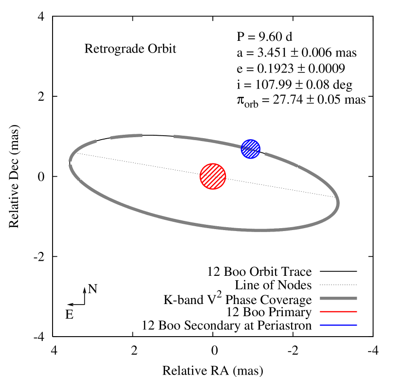
Figure 1: Visual Orbit of 12 Boötis. The relative visual orbit model of 12 Boo is shown, with the primary and secondary objects rendered at T₀ (periastron). The heavy lines along the relative orbit indicate areas where we have phase coverage in our $K$-band PTI data (they are not separation vector estimates); our data cover essentially all phases of the orbit, leading to a reliable orbit determination. Component diameter values are estimated (see discussion in § 4), and are rendered to scale.

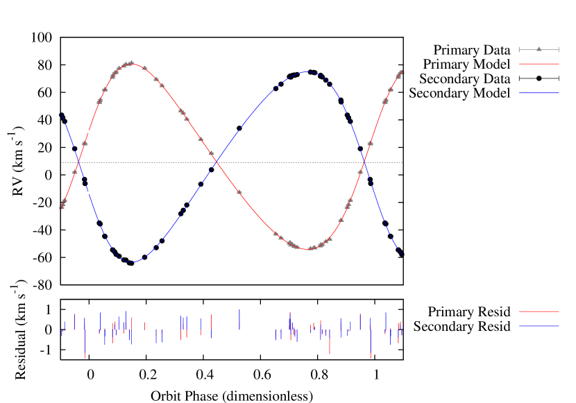
Figure 2: Radial Velocity Orbit of 12 Boo. A phase-folded plot of our radial velocity data and RV predictions from our Full-Fit solution (Table 4). The lower frame gives RV residuals to the model fit.

Tables 2 and 2 list the constituent set of $V^{2}$ and RV measurements in our 12 Boo dataset, and residuals (in a datum minus model sense) between the observables and predictions based on the best-fit integrated orbit model (our “Full-Fit” model, Table 4) for 12 Boo. Figures 2 and 3 illustrate the results of our orbit modeling for 12 Boo. Figure 2 depicts phased RV measurements and the primary and secondary radial velocity orbits from our integrated model. Inset in the lower frame are phased velocity residuals (data minus model). Figure 3 depicts the phase coverage of our visibility and radial velocity data, and the statistics of our modeling residuals. The agreement between our various data and our orbit model is excellent; our full-fit solution results in total chi-squared per of degree of freedom in our fit of 0.85 (suggestive that we may have overestimated our measurement errors). The resulting rms $V^{2}$ and RV measurement residuals from our model are 0.027 and 0.49 km s^-1 respectively.

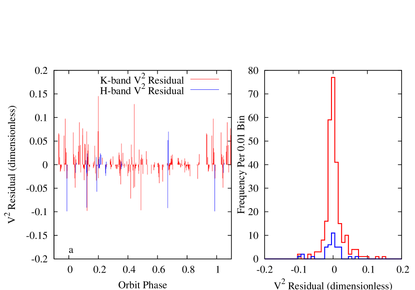
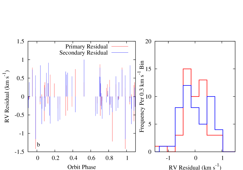
Figure 3: Orbit Fit Residuals for 12 Boo. a: Orbit phase plots of $K$ and $H$-band V² fit residuals, and residual histograms for the “Full-Fit” orbit model. b: Orbit phase plots of radial velocity fit residuals, and residual histograms for the “Full-Fit” orbit model. (Table 4).

Orbit models for 12 Boo are summarized in Table 4, including spectroscopic orbit parameters from DU99, the integrated model from Paper 1, and our present visual, spectroscopic, and integrated orbit models. In particular we list the results of separate fits to only our $K$-band $V^{2}$ data (our “$V^{2}$ Only” solution), our double-lined radial velocity data (our “RV Only” solution), and a simultaneous fit to our $V^{2}$ and RV data (our “Full-Fit” solution) – all with component diameters constrained as noted above. For the orbit parameters we have estimated from our visibility data we list a total one-sigma error in the parameter estimate, including errors in the parameter estimates from statistical (measurement uncertainty) and systematic error sources. In our analysis the dominant forms of systematic error are: (1) uncertainties in the calibrator angular diameters (Table 1); (2) uncertainty in the center-band operating wavelength ($\lambda_{0}\approx$ 2.2 $\mu$m), taken to be 10 nm ($\sim$0.5%); (3) the geometrical uncertainty in our interferometric baseline ( $<$ 0.01%); and (4) uncertainties in ancillary parameters constrained in our orbit fitting procedure (i.e. the angular diameters in all solutions involving interferometry data). For example, our angular semi-major axis error is completely dominated by the operating wavelength uncertainty – the statistical error is a factor of five smaller.

In addition to the overall orientation, the NPOI data have been used to estimate the component in-band intensity ratio, constraining to the relevant orbital parameters from the “Full Fit” solution. The 750 nm intensity ratio is constrained by the NPOI closure phases and the ratio of the maximum to minimum visibility amplitudes. As there were small systematic, but wavelength-independent deviations of the measured amplitudes on individual baselines from the model, we allowed the amplitude calibration to vary during the fitting (while the phases are unaffected). The resulting component intensity ratio (0.614 $\pm$ 0.038) yields a magnitude difference $\Delta M$ = 0.53 $\pm$ 0.07 at 750 nm. This value agrees well with the relatively increasing secondary contribution seen in the other observed bands ($K$, $H$, and $V$; component magnitude differences in all observed bands are given in Table 4), and is understood in the context of the slightly higher temperature of the 12 Boo secondary compared to the primary (§2).

Table 4: Orbital Parameters for 12 Boo. Summarized here are the apparent orbital parameters for the 12 Boo system as determined by DU99, Paper 1, and present results. We give three separate fits to our data: $K$-band V² only, RV only, and integrated (“Full Fit”). Note that $\omega_{A}$ refers to the argument of periapsis of the primary component, and (unlike Paper 1) $\Omega$ values are the position angle of the ascending node.

Orbital	DU99	Paper 1	PTI & CfA
Parameter		Full-Fit	$K$-band V2 Only	RV Only	Full-Fit
Period (d)	9.6046	9.604565	9.604638	9.6045518	9.6045492
	$\pm$ 1 $\times$ 10-4	$\pm$ 1.0 $\times$ 10-5	$\pm$ 5.9 $\times$ 10-5	$\pm$ 8.6 $\times$ 10-6	$\pm$ 7.6 $\times$ 10-6
T0 (MJD)	48990.29	51237.779	51237.7596	51237.7798	51237.7729
	$\pm$ 0.03	$\pm$ 0.024	$\pm$ 0.0086	$\pm$ 0.0090	$\pm$ 0.0051
$e$	0.193	0.1884	0.1895	0.19256	0.19233
	$\pm$ 0.004	$\pm$ 0.0022	$\pm$ 0.0022	$\pm$ 0.00099	$\pm$ 0.00086
K1 (km s-1)	67.11 $\pm$ 0.41	67.84 $\pm$ 0.31		67.320 $\pm$ 0.090	67.302 $\pm$ 0.087
K2 (km s-1)	70.02 $\pm$ 0.48	69.12 $\pm$ 0.48		69.38 $\pm$ 0.10	69.36 $\pm$ 0.10
$\gamma$ (km s-1)	9.29 $\pm$ 0.19	9.11 $\pm$ 0.13		9.550 $\pm$ 0.051	9.551 $\pm$ 0.051
$\omega_{A}$ (deg)	286.19 $\pm$ 1.31	287.03 $\pm$ 0.75	286.85 $\pm$ 0.35	286.92 $\pm$ 0.35	286.67 $\pm$ 0.19
$\Omega$ (deg)		79.83 $\pm$ 0.45	80.49 $\pm$ 0.12		80.291 $\pm$ 0.079
$i$ (deg)		108.58 $\pm$ 0.36	108.15 $\pm$ 0.12		107.990 $\pm$ 0.077
$a$ (mas)		3.392 $\pm$ 0.050	3.449 $\pm$ 0.018		3.451 $\pm$ 0.018
$\Delta K_{\rm CIT}$ (mag)		0.618 $\pm$ 0.022	0.593 $\pm$ 0.006		0.589 $\pm$ 0.005
$\Delta H_{\rm CIT}$ (mag)		0.566 $\pm$ 0.066			0.560 $\pm$ 0.020
$\Delta M_{750nm}$ (mag)					0.53 $\pm$ 0.07
$\Delta V$ (mag)		0.5 $\pm$ 0.1			0.485 $\pm$ 0.017
$\chi^{2}$/DOF		1.2	0.82	1.0	0.85
$\overline{|R_{V^{2}}|}$/$\sigma_{V^{2}}$		0.023	0.017/0.027		0.017/0.027
$\overline{|R_{RV}|}$/$\sigma_{RV}$ (km s-1)	0.90	1.7		0.39/0.49	0.40/0.49

4 Physical Parameters

Physical parameters derived from our 12 Boo “Full-Fit” integrated visual/spectroscopic orbit are summarized in Table 5. Notable among these is the high-precision determination of the component masses for the system, a virtue of the favorable geometry of the orbit and the quality of the visibility and radial velocity datasets. We estimate the masses of the primary and secondary components as 1.4160 $\pm$ 0.0049 and 1.3740 $\pm$ 0.0045 M_☉, respectively. These are in good agreement (approximately 1.0 and 1.7 sigma for the primary and secondary respectively) with the component mass estimates given in Paper 1.

The Hipparcos catalog lists the parallax of 12 Boo as 27.27 $\pm$ 0.78 mas (ESA, 1997). The distance determination to 12 Boo based on our orbital solution is 36.08 $\pm$ 0.19 pc, corresponding to an orbital parallax of 27.72 $\pm$ 0.15 mas, consistent with the Hipparcos result at 1.7% and 0.6-sigma.

A number of metallicity estimates for 12 Boo exist in the literature that appear to indicate a composition near solar. Photometric estimates by Duncan (1981), Balachandran (1990), and Nordström et al. (2004) give [Fe/H] values of $-0.03$, $+0.12\pm 0.12$, and $-0.06$, respectively, and are based on Strömgren $uvby\beta$ or $\delta(U-B)_{0.6}$ indices. Although the object was recognized as a binary in these investigations, no corrections for this were made. The effect is expected to be small in any case, as the two components have very similar temperatures. Spectroscopic determinations of the metallicity have been reported by Balachandran (1990) and Lèbre et al. (1999) as [Fe/H] = $-0.03\pm 0.09$ and [Fe/H] = $-0.1\pm 0.1$, respectively. Once again the binary nature of 12 Boo was known to these investigators, although Balachandran (1990) reported not detecting the secondary in their spectra. The effect would be to make the spectral lines appear somewhat weaker, since the secondary ($L_{\rm sec}/L_{\rm prim}=0.64$) would tend to fill in the lines of the primary. Overall there is good agreement in that all these studies place the metallicity of 12 Boo within 0.1 dex of solar. This metallacity range is an important constraint we use below in the comparison with stellar evolution models.

Table 5: Physical Parameters for 12 Boo. Summarized here are the physical parameters for the 12 Boo system as derived primarily from the “Full-Fit” solution orbital parameters in Table 4. For comparison we have also given the corresponding parameter values from Paper 1 (offset in brackets and italics). We have used system photometry in $K$ and $H$ from Paper 1, and in $V$ from Mermilliod & Mermilliod (1994).

Physical	Primary (A)	Secondary (B)
Parameter	Component	Component
a (10-2 AU)	6.1305 $\pm$ 0.0084 [6.205 $\pm$ 0.032]	6.3179 $\pm$ 0.0092 [6.322 $\pm$ 0.046]
Mass (M☉)	1.4160 $\pm$ 0.0049 [1.435 $\pm$ 0.023]	1.3740 $\pm$ 0.0045 [1.408 $\pm$ 0.020]
Sp Type (Barry 1970)	F9 IVw
System Distance (pc)	36.08 $\pm$ 0.19 [36.93 $\pm$ 0.56]
$\pi_{orb}$ (mas)	27.74 $\pm$ 0.15 [27.08 $\pm$ 0.41]
Bolometric Flux (10-7 erg cm-2 s-1)	3.074 $\pm$ 0.021
Teff (K)	6130 $\pm$ 100	6230 $\pm$ 150
Bolometric Flux (10-7 erg cm-2 s-1)	1.92 $\pm$ 0.07	1.16 $\pm$ 0.17
Model Diameter (mas)	0.638 $\pm$ 0.025	0.480 $\pm$ 0.039
Radius (R⊙)	2.474 $\pm$ 0.095	1.86 $\pm$ 0.15
log g	3.802 $\pm$ 0.033	4.036 $\pm$ 0.070
MK-CIT (mag)	1.261 $\pm$ 0.034 [1.200 $\pm$ 0.038]	1.851 $\pm$ 0.034 [1.818 $\pm$ 0.039]
MH-CIT (mag)	1.322 $\pm$ 0.042	1.882 $\pm$ 0.043
MV (mag)	2.581 $\pm$ 0.014 [2.524 $\pm$ 0.052]	3.066 $\pm$ 0.036 [3.024 $\pm$ 0.077]
$V$-$K$ (mag)	1.293 $\pm$ 0.032	1.188 $\pm$ 0.047

Component Diameters, Effective Temperatures, and Radii

The “effective” angular diameter of the 12 Boo system has been estimated using the infrared flux method (IRFM) by Blackwell and collaborators (Blackwell et al., 1990; Blackwell & Lynas-Gray, 1994) at approximately 0.8 mas. At this size neither of the 12 Boo components are resolved by PTI, and we must resort to model diameters for the component stars. Following Blackwell, we estimate 12 Boo component diameters through bolometric flux and effective temperature ($T_{\rm eff}$) arguments. Blackwell & Lynas-Gray (1994) list the bolometric flux of the 12 Boo system at 3.11$\times$10^-7 erg cm^-2 s^-1, and $T_{\rm eff}$ as 6204 K, both quoted without error estimates. Similarly we have analyzed archival photometry available from SIMBAD, 2MASS, and Paper 1 using an empirical model atmosphere for a solar-metallicity F8 IV star taken from Pickles (1998). Figure 4 depicts the results of this SED modeling, resulting in a bolometric flux estimate of 3.074 $\pm$ 0.021 $\times$10^-7 erg cm^-2 s^-1 – in reasonable agreement with the Blackwell & Lynas-Gray (1994) result, and providing a plausible error estimate.

As a check on our spectroscopic effective temperature estimates we have made additional estimates the 12 Boo component effective temperatures from the component colors. The interferometric and spectroscopic observations provide $V$ - $K$ color indices for the components individually (Table 5). With these color indices we have used effective temperature/color calibrations published by Blackwell & Lynas-Gray (1994) and Alonso et al. (1996) (with the component $K$ magnitudes transformed to the Johnson system). The resulting component effective temperature estimates are in excellent agreement with our adopted spectroscopic values (§2, Table 5).

Estimating the bolometric flux ratio from the observed $K$-band flux ratio and component effective temperatures provide bolometric flux estimates for the two components individually (Table 5), and these along with the effective temperatures allow us to estimate angular diameters of 0.638 $\pm$ 0.025 and 0.480 $\pm$ 0.039 mas for the primary and secondary components respectively. At the distance estimate to 12 Boo these model angular diameters correspond to model component linear radii of 2.474 $\pm$ 0.095 and 1.86 $\pm$ 0.15 R_☉ for the primary and secondary components respectively. Finally, coupled with our component masses we find (log) surface gravities of 3.802 $\pm$ 0.033 and 4.036 $\pm$ 0.070 dex. All these estimates are in good agreement with (and more precise than) the results from Paper 1. These linear radii estimates are roughly a factor of two smaller than the putative Roche lobe radii for these two stars (Iben, 1991, Eq. 1), making significant mass transfer unlikely at this stage of system evolution.

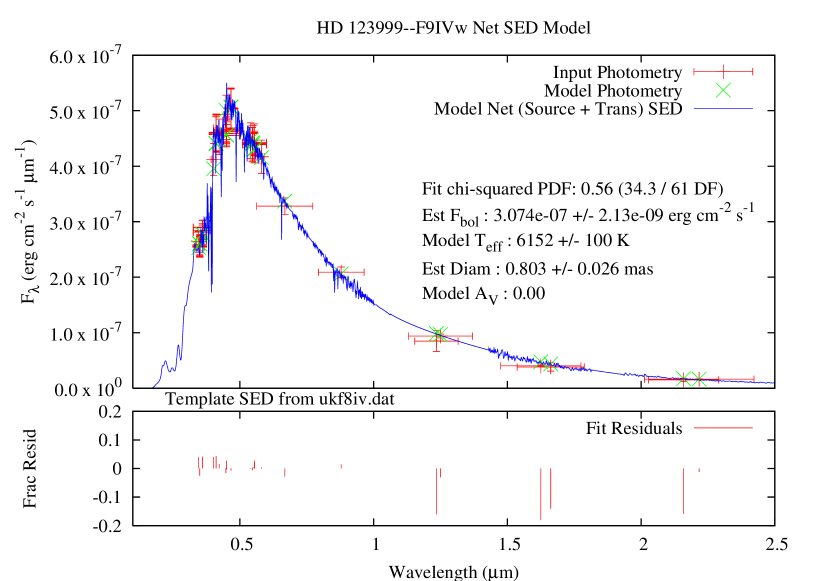
Figure 4: Spectral Energy Distribution Model for 12 Boo. Here a template Spectral Energy Distribution (SED) template from Pickles (1998) has been fit to archival photometry from SIMBAD, 2MASS, and Paper 1 to estimate the bolometric flux for 12 Boo system (Table 5).

Component Rotation

Tidal interaction theory predicts that in short-period binary systems the components gravitationally interact so as to circularize the orbit and synchronize the component rotations to the orbital period (Zahn, 1977; Hut, 1981); these predictions are borne out in observation (e.g. Duquennoy & Mayor, 1991). The circularization and synchronization phenomena necessarily require an energy dissipation mechanism, generally thought to be associated with convection in the outer envelopes of cool stars such as giants (Verbunt & Phinney, 1995).

Paper 1 noted that 12 Boo is interesting from a tidal interaction perspective: despite the relatively short orbital period the system orbit is modestly eccentric (Table 4). The component masses indicate both components were around F1 – F3 at their initial appearance on main sequence; the putative reason for the remnant orbital eccentricity is the lack of strong convection in the atmospheres during the components’ main-sequence lives. However, as the 12 Boo components evolve off the main sequence their atmospheres become much more convective, and tidal circularization and synchronization should begin. Once the component atmospheres become fully convective the timescale for rotation synchronization will be short ($\sim$ 1 Myr for the primary; Paper 1).

Several recent measurements of the rotation $v\sin i$ of 12 Boo components exist, offering the possibility to assess whether the two components are currently synchronously rotating. These 12 Boo component rotation measurements are summarized Table 6. As in Paper 1, the consensus remains that both 12 Boo components appear to be rotating consistent with synchronous rates. Within the errors and the scatter of the measurements the secondary $v\sin i$ is also consistent with the pseudosynchronous rate (synchronous with the orbital motion at periastron; Hut 1981), while the primary appears to be rotating marginally slower than the pseudosynchronous rate.

	Primary	Secondary
	$v\sin i$	$v\sin i$
	(km s-1)	(km s-1)
Balachandran (1990)	10 $\pm$ 3
De Medeiros et al. (1997)	12.7 $\pm$ 1
DU99	12.5 ($\pm$ 1)	9.5 ($\pm$ 1)
Paper 1	13.1 $\pm$ 0.3	10.4 $\pm$ 0.3
Shorlin et al. (2002)	14.0 $\pm$ 3.0	12.0 $\pm$ 3.0
Reiners & Schmitt (2003)	15.0 $\pm$ 1.0
This work	14.0 $\pm$ 1.0	12.0 $\pm$ 1.0
Model Synch Rotation	12.4 ($\pm$ 1.1)	9.3 ($\pm$ 0.8)
Model Pseudo-Synch Rotation	15.2 ($\pm$ 1.4)	11.4 ($\pm$ 1.0)

Table 6: $v\sin i$ Measurements for 12 Boo Components. Summarized here are recent $v\sin i$ measurements for the 12 Boo system components, including this work. For references where a single $v\sin i$ measurement is listed we have assumed this pertains to the primary component. DU99 does not list errors for their component $v\sin i$ estimates; we have arbitrarily taken 1 km s^-1 so as to be consistent with the characteristic accuracies of earlier CORAVEL determinations (see discussions in De Medeiros et al., 1996, 1997). For comparison we give model estimates of $v\sin i$ for synchronous and pseudosynchronous rotation of the two components given the physical sizes discussed in § 4. Both 12 Boo components would appear to be rotating at rates consistent with synchronous rotation.

5 Comparisons With Stellar Models

With our estimates of the component masses, absolute magnitudes, color indices, and effective temperatures derived from our measurements and orbital solution (Table 5), we proceed in this section to examine the 12 Boo components in the context of recent stellar evolution models.

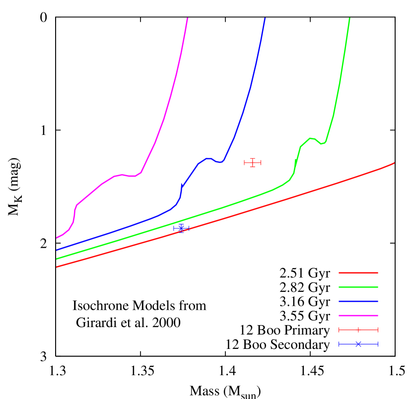
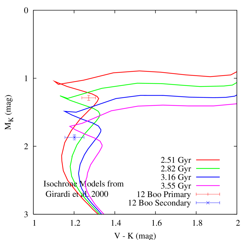
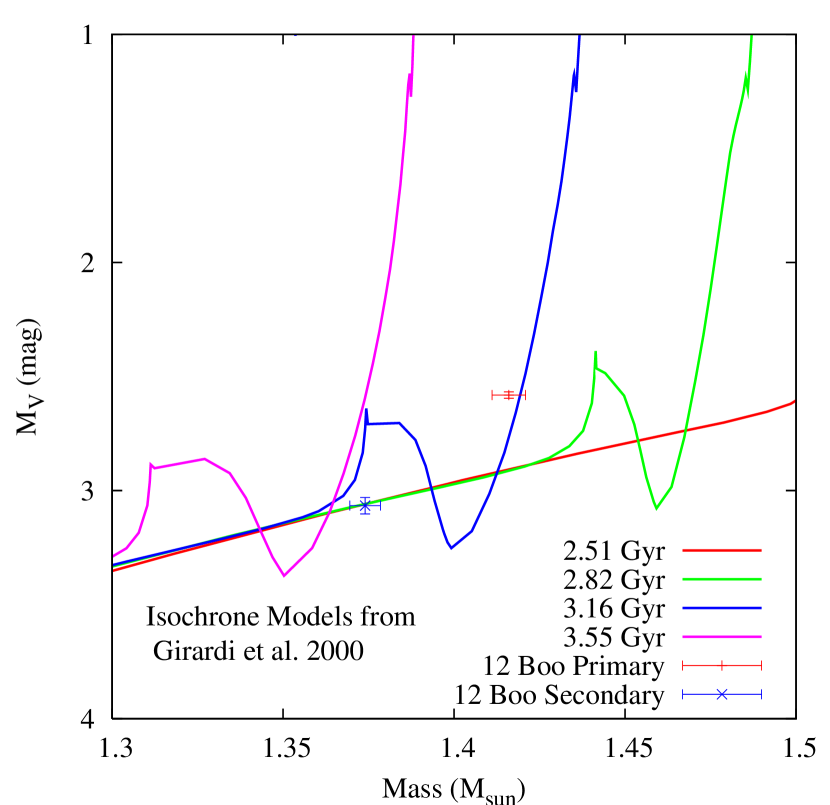
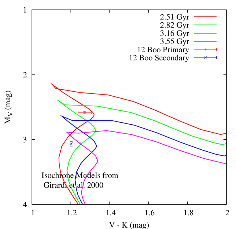
Figure 5: Comparison of the 12 Boo Component Parameters with Girardi et al. 2000 (G2000) Stellar Models. Comparisons between our observed 12 Boo component parameters and G2000 models are shown in observable mass-magnitude and color-magnitude spaces.

In Paper 1 we compared the measurements for the 12 Boo components with models from the Padova series by Bertelli et al. (1994). Since then the input physics of these particular models has been updated mainly by incorporating improvements in the equation of state and in the opacities, as described by Girardi et al. (2000, hereafter G2000). In Figure 5 the observed properties of the 12 Boo components are shown against four isochrones for solar metallicity from G2000, in various planes. The panels on the left show the $V$ and $K$ absolute magnitudes versus mass (diagrams for $H$ are similar and are not shown here). (For purposes of model comparisons the component infrared magnitudes have been transformed from the CIT to the Johnson system using color conversions from Bessell & Brett, 1988). No single isochrone appears to fit the observations within the error bars. The diagrams on the right suggest that an isochrone between 2.5 Gyr and 2.8 Gyr might provide a good fit in the color-magnitude plane, with both stars located near the end of their hydrogen-burning phase. Paper 1 reached a similar conclusion on the system age estimate based on Padova models. However, as indicated by the left-hand figures the model masses for such an age would not agree with the measured component parameters.

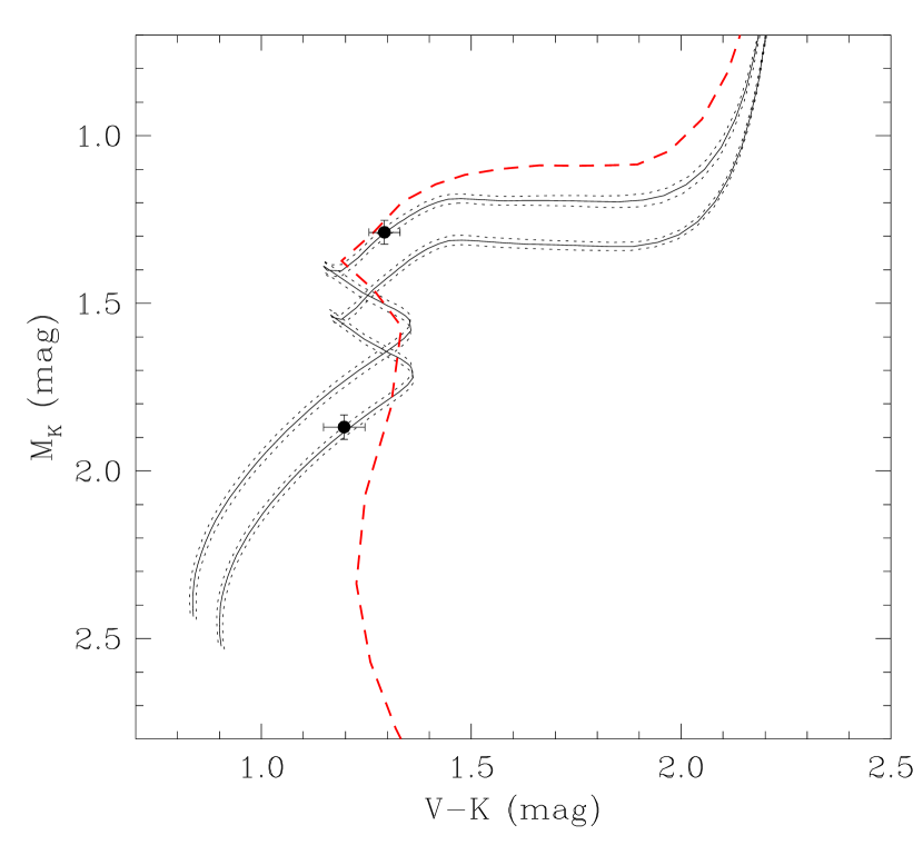
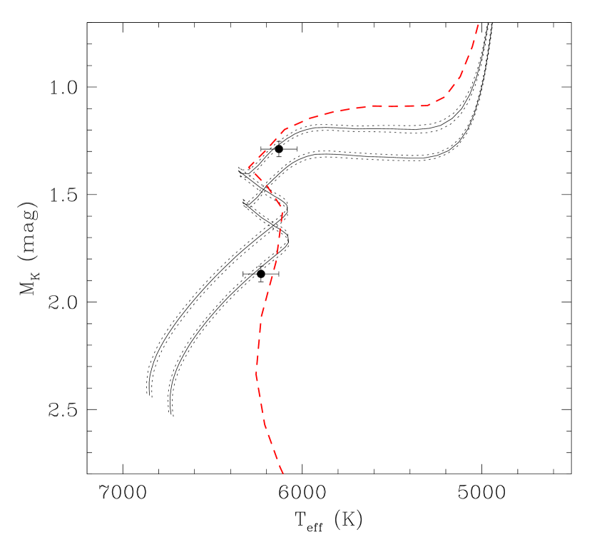
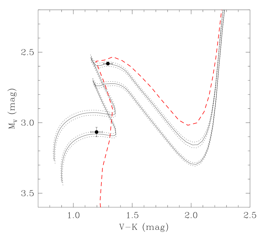
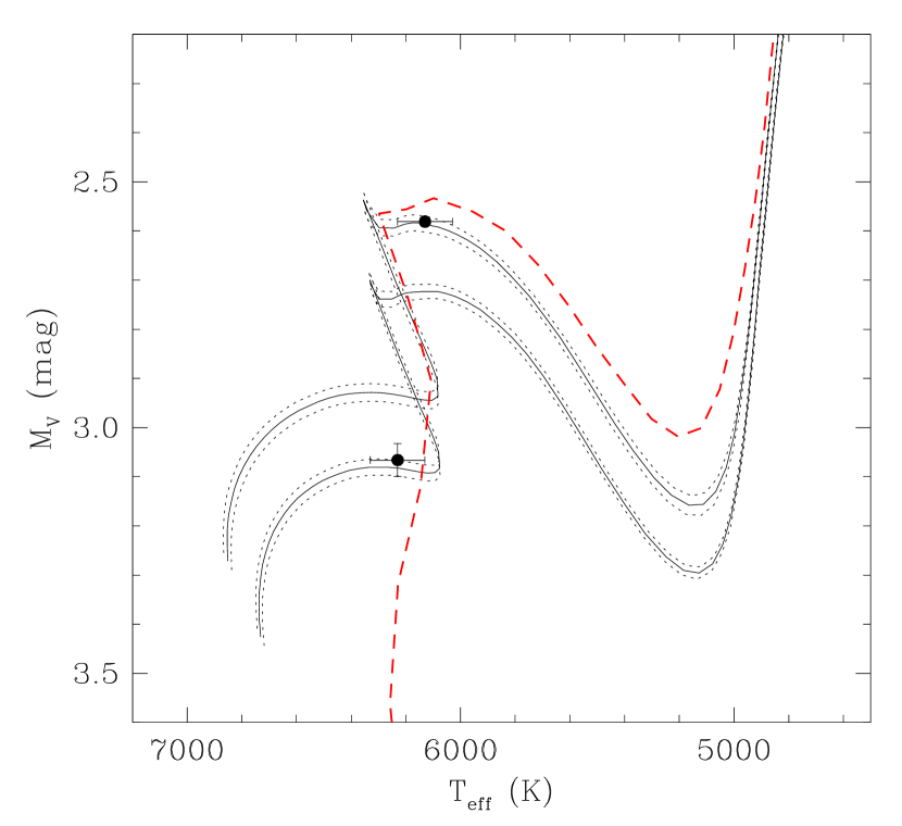
Figure 6: Comparison of the 12 Boo Component Parameters with Yonsei-Yale (Y²) Stellar Models. Comparisons between our observed 12 Boo component parameters and Y² models are shown in color-magnitude and temperature-magnitude spaces. The figures give mass tracks computed for the particular masses of the 12 Boo components (shown in black including mass uncertainties), and the best-fit single isochrone to the parameters of both components (age of 3.2 Gys – shown in the red dashed line).

Figure 6 compares the observed quantities to models from the Yonsei-Yale (Y²) collaboration (Yi et al., 2001; Demarque et al., 2004). The Y² models use similar physics to G2000, but differ in a number of details including the radiative opacities, the equation of state, the treatment of convective core overshooting, and the implementation of helium and heavy element diffusion (not accounted for in G2000). In this case we show evolutionary tracks for the exact component masses determined from the physical orbit (Table 5), using an interpolation routine described by Yi et al. (2003). Absolute magnitudes in $V$ and $K$ are displayed against both $V-K$ and effective temperature as estimated from our spectra, so that each panel displays the constraint from three observables at the same time (shown with their uncertainties) rather than two as in the previous figure. The one-sigma mass uncertainties are indicated by the dotted lines bracketing the tracks. To show the constraint on coevality, which we assume to hold for this binary, an isochrone from the same series of models is also represented in each panel. An age of 3.2 Gyr provides the best overall fit to the observations; this is significantly older than the system age estimate from Paper 1 based on Bertelli models. As mentioned in § 4, the metallicity determinations in the literature suggest a near-solar composition for 12 Boo. The Y² models seem to agree with that assessment; in surveying a range of metallicities allowed by previous studies we found the best agreement between our observational parameters and the model predictions at solar abundance ($+0.0$ dex/Z=0.01812 in Y² models). While our estimates of the surface gravities and absolute radii for the stars rely not on the physical orbit but on other radiative properties, they do enter weakly into the orbital solution (through the component angular diameters) as well as our spectroscopic estimate of the effective temperatures (§ 2). The comparison of our inferred $\log g$ and radius (Table 5) values with the Yi et al. (2003) models is shown in Figure 7.

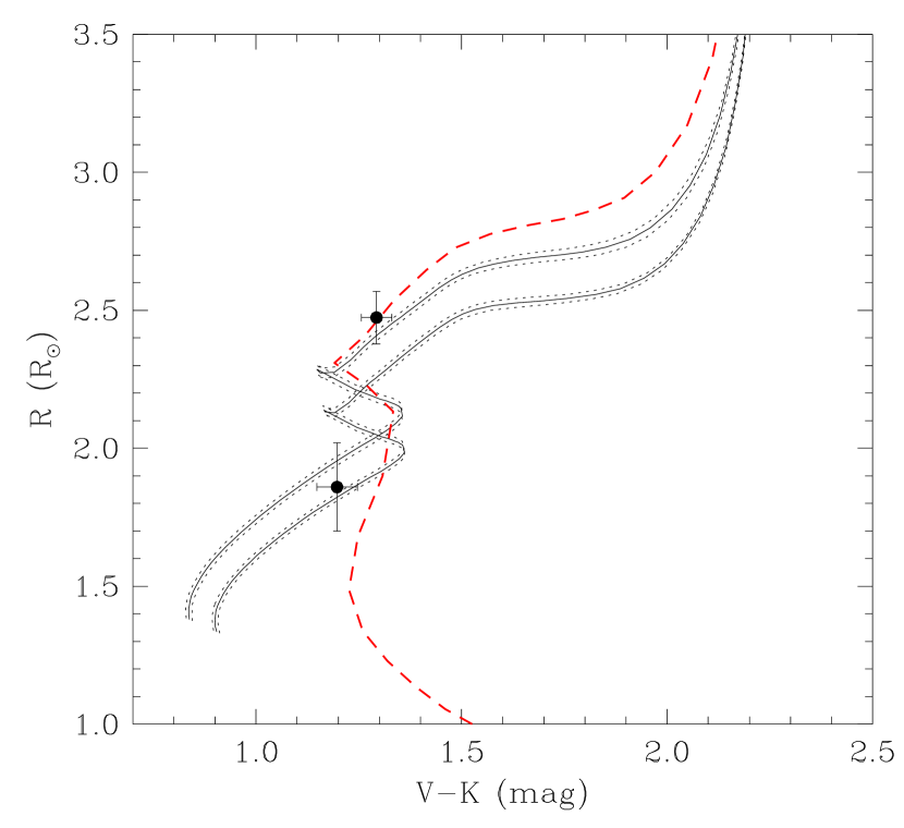
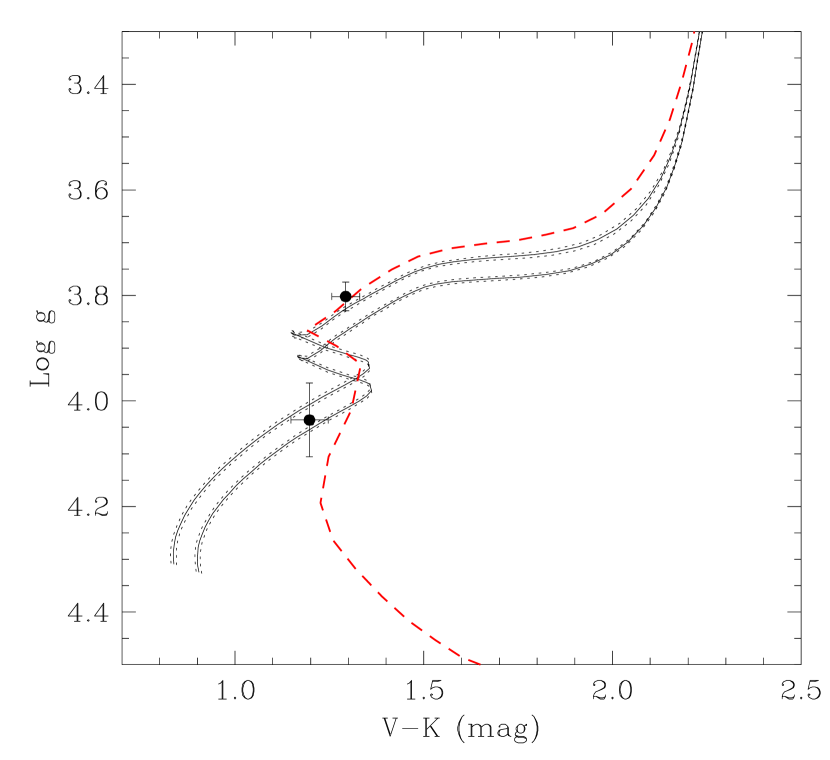
Figure 7: Comparison of the 12 Boo Component Radii with Y² Models. Comparisons of the estimated component radii and surface gravity with predictions from the Y² models. Mass tracks for the two system components are given in solid black lines, with the 3.2 Gyr isochrone is given in the red dashed line.

Figure 6 suggests the secondary of 12 Boo is comfortably in the main-sequence stage, while the primary would appear to be near the beginning of the rapid phase of evolution where it burns hydrogen in a shell – the so-called Hertzsprung gap. The duration of this phase is only about 4% of the main-sequence lifetime for a star of this mass. Although it is a priori unlikely that we would find a star in this state, the possibility can certainly not be excluded (e.g. see Andersen et al, 1990; Fekel et al, 2001; Parsons, 2004). However, we note that a minor increase in the amount of convective core overshooting (a free parameter in the models) could easily extend the main sequence enough to bring agreement with the observations for the primary star, placing it at the end of the hydrogen-burning phase rather than in the Hertzsprung gap. The treatment of overshooting in these models follows the recent prescription described by Demarque et al. (2004), in which the overshooting parameter $\Lambda_{\rm OS}$ (in units of the pressure scale height $H_{p}$) increases gradually from 0.00 to 0.20 as a function of mass in the regime in which a convective core develops ($M_{crit}^{conv}\sim 1.2$ M_☉ for solar composition). This was deemed a more realistic approximation than that adopted in the previous release of the Y² models (Yi et al., 2001), in which $\Lambda_{\rm OS}=0.00$ for masses up to $M_{crit}^{conv}$ and $\Lambda_{\rm OS}=0.20$ for larger masses. Given the mass of the 12 Boo primary (Table 5), the interpolation performed to produce the track for Figure 6 results in an effective overshooting parameter of approximately 0.16. With the old prescription the overshooting would be 0.20. In Figure 8 we illustrate the effect of changing $\Lambda_{\rm OS}$ by showing the primary tracks for both values, where the solid curve is the same model as in Figure 6 (new overshooting prescription). As expected the track corresponding to $\Lambda_{\rm OS}=0.20$ (old prescription) has a more extended main sequence reaching slightly cooler temperatures, and comes closer to matching the observed location of 12 Boo A at the very end of the core burning phase. While both sets of model predictions are consistent with the observed properties of the 12 Boo primary, it seems a priori more likely that the star is at the end of its main-sequence life. If the 12 Boo primary is at the end of main sequence, the observations would seem to place fairly tight constraints on overshooting that suggest somewhat larger values of $\Lambda_{\rm OS}$ than adopted by Demarque et al. (2004).

Figure 8: Effects of Different Convective Overshooting Parameters on the Y² Models

The apparent agreement between Y² model predictions and our measurements is in contrast to the apparent disagreement of our results with the Padova/G2000 model series. The differences between the Y² and Padova models are more directly appreciated in Figure 9, where we show 2.82 Gyr ($\log age=9.45$) isochrones from both series for the same (solar) metallicity. From top to bottom we depict the isochrones from the purely theoretical plane (luminosity versus $T_{eff}$) to the purely observational plane (absolute magnitude versus $V-K$ color). While there is excellent agreement for unevolved stars in the top two diagrams (lower main sequence), the end of the main-sequence region highlights the subtle differences that have to do with the details in the input physics. In the lower panel the discrepancies extend also to the unevolved stars; this is due to differences in the color-temperature calibrations between the models. Over the temperature range shown in the figure the Padova isochrone relies on color and bolometric correction tables based on theoretical model atmospheres (see Bertelli et al., 1994), while the Y² model relies on semi-empirical tables by Lejeune, Cuisinier, & Buser (1998).

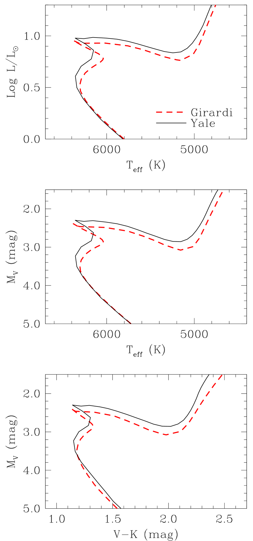
Figure 9: Direct Comparisons of G2000 and Y² Models in Theoretical and Observational Color-Magnitude Spaces. The three panels show comparisons of 2.82 Gyr solar metallicity isochrones near the main-sequence end from G2000 (red) and Y² (black) in theoretical (Luminosity vs. T_eff – top), semi-observational (M_V vs. T_eff – middle), and observational (M_V vs. $V-K$ – bottom) color-magnitude spaces.

6 Summary and Discussion

By virtue of our interferometric resolution and the precision of the radial velocity data we are able to determine an accurate physical orbit for 12 Boo, resulting in accurate physical parameters for the 12 Boo constituents and an accurate system distance. Our 12 Boo distance estimate is in excellent agreement with the Hipparcos determination. Our finding of unexpectedly large relative $K$, $H$, and $V$-magnitude differences in the two nearly-equal mass 12 Boo components is understood in the context that the system is in a unique evolutionary state, with the primary component apparently making its transition off the main sequence. 12 Boo component rotation measurements are consistent with synchronous rotation for the system components, and at least the primary is less consistent with pseudosynchronous rotation.

The results of comparing the 12 Boo components with stellar models are mixed. While we see relatively good agreement between the component physical parameters and the Y² evolutionary (mass) tracks, the agreement with the G2000 isochrones is not nearly as good. Further, the discrepancy seems to be intrinsic; Figure 9 illustrates that fundamental differences exist between the Y² and G2000 models in both theoretical and observational spaces near the end of the main sequence. Our measured 12 Boo component parameters are clearly in much better agreement with the Y² model predictions for intermediate-mass stars near the end of the main sequence.

Further, it is interesting to note that the agreement between our observations and the Y² mass tracks is significantly better than the agreement with the best-fit Y² isochrone at 3.2 Gyr. Presumably the 12 Boo components must be coeval, so the larger mismatch in the isochrone prediction must be indicative of a remaining discrepancy between the observations and Y² models. This discrepancy is illustrated in Figure 10, which depicts the 12 Boo components and their mass tracks in the same observational color-absolute magnitude spaces given in Figure 6. The left panels in Figure 10 focus on the observed component parameters and Y² mass tracks, and in particular indicate the ages on the mass tracks that best match the component parameters. We find the Y² tracks would indicate best-match ages of 3.25 and 2.91 Gyrs for the primary and secondary components respectively. The right panels in Figure 10 show these same spaces with Y² isochrones computed for the specific best-match component ages. Presumably this apparent discrepancy in the component ages cannot be physical. It seems likely that the unique evolutionary state of 12 Boo could provide important observational constraints on the physical evolution of intermediate-mass stars making their transition off the main sequence.

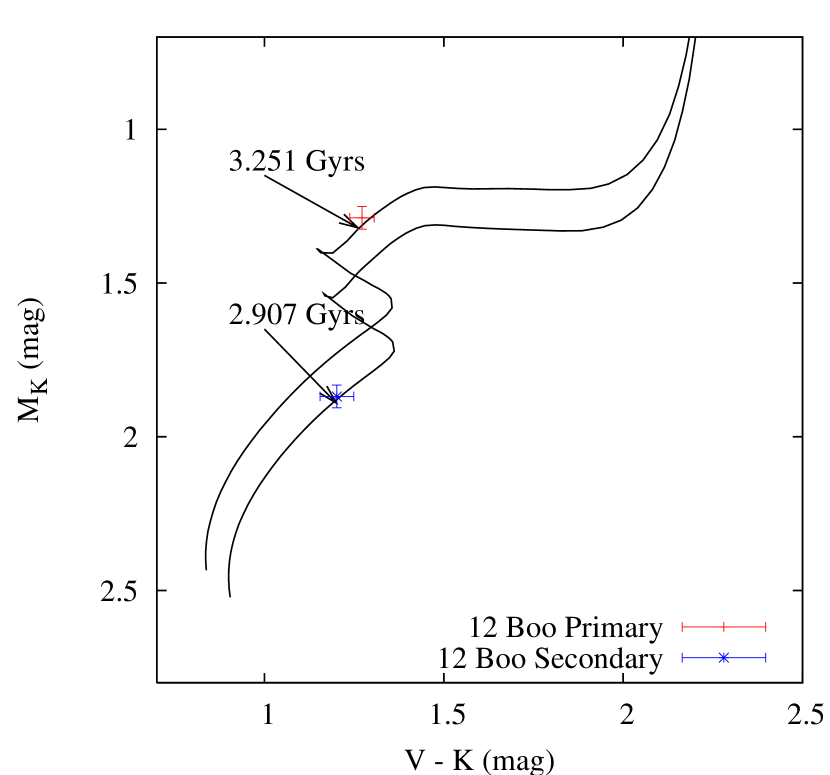
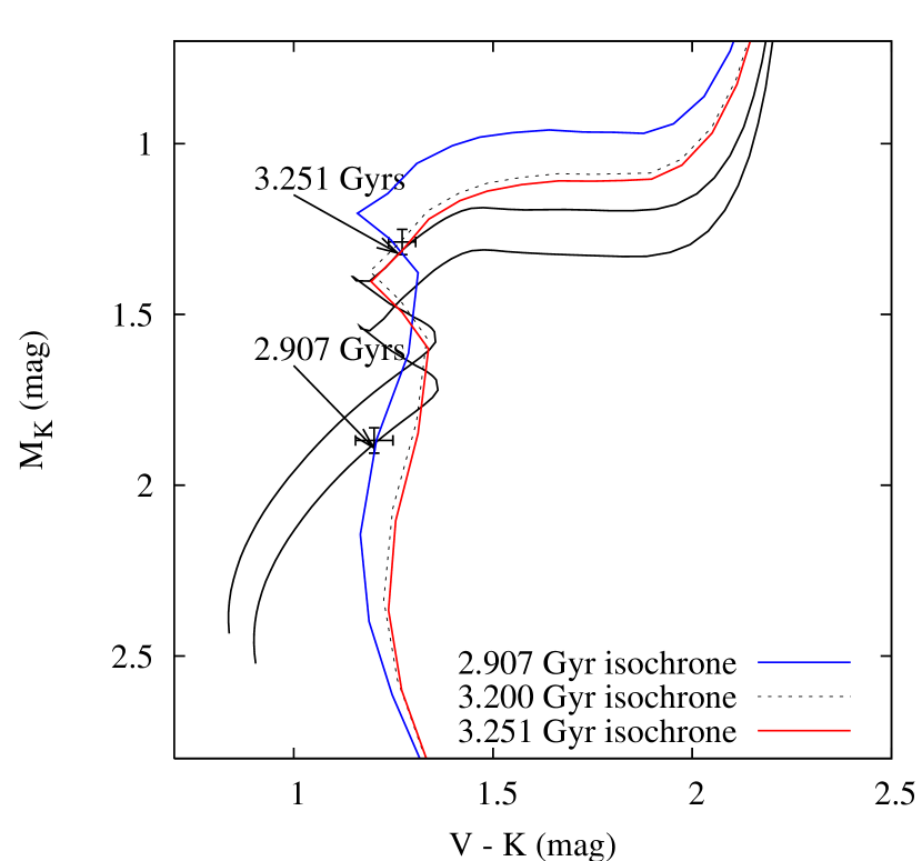
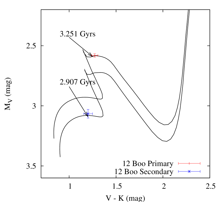
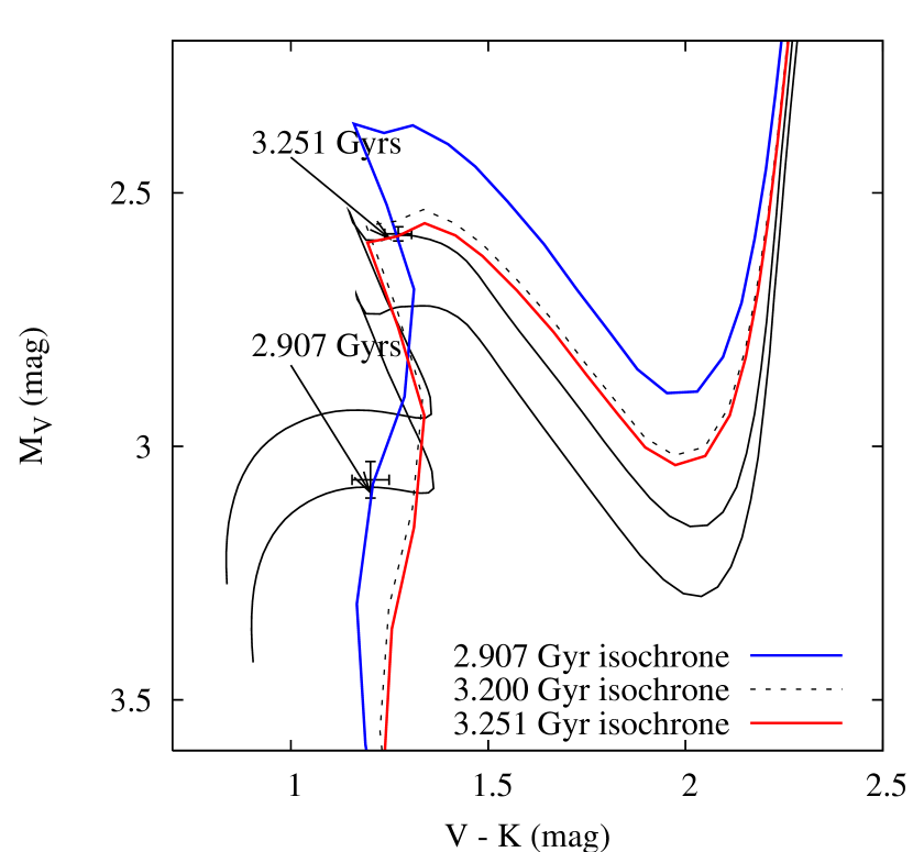
Figure 10: 12 Boo Component Age Estimates from Y² Stellar Models. The left panels indicate best-match component ages estimated from Y² mass tracks in observational $M_{K}$ and $M_{V}$ vs $V-K$ planes. The right panels show the same quantities, superimposing Y² isochrones computed for these best-match component age estimates. Presumably the apparent 340 My component age discrepancy cannot be physical.

Finally, Figures 6, 7, and 10 lead to the tempting inference that the 12 Boo primary is early in its first transition across the Hertzsprung gap to the base of the red giant branch. However, as discussed in § 5, Figure 8 shows that at the apparent evolutionary state of the 12 Boo primary relatively small changes in the physics of the stellar models can make significant changes in the model predictions. Particularly coupled with the apparent age discrepancy in the 12 Boo components indicated by the models, caution suggests that a Hertzsprung-gap interpretation for the 12 Boo primary should be provisional only.

References

- Abt & Levy (1976) Abt, H. and Levy, S. 1976, ApJS 30, 273.
- Alonso et al. (1996) Alonso, A., Arribas, S., and Martinez-Roger, C. 1996, A&A313, 873.
- Alonso et al. (1999) Alonso, A., Arribas, S., and Martinez-Roger, C. 1999, A&AS140, 261.
- Andersen et al (1990) Andersen, J., Nordström, B., & Clausen, J. V. 1990, ApJ, 363, L33
- Armstrong et al. (1992) Armstrong, J.T. et al. 1992, AJ 104, 2217.
- Armstrong et al. (1998) Armstrong, J.T. et al. 1998, ApJ 496, 550.
- Balachandran (1990) Balachandran, S. 1990, ApJ 354, 310.
- Barry (1970) Barry, D. 1970, ApJS 19, 281.
- Bertelli et al. (1994) Bertelli, G., Bressan, A., Chiosi, C., Fagotto, F., and Nasi, E. 1994 (B94), A&AS 106, 275.
- Bessell & Brett (1988) Bessell, M. and Brett, J. 1988, PASP 100, 1134.
- Blackwell et al. (1990) Blackwell, D., Petford, A., Arribas, S., Haddock, D., and Selby, M. 1990, A&AS 232, 396.
- Blackwell & Lynas-Gray (1994) Blackwell, D., and Lynas-Gray, A. 1994, A&A 282, 899.
- Boden et al. (1998) Boden, A.F. et al. 1998, Proc. SPIE 3350, 872.
- Boden et al. (1999a) Boden, A.F. et al. 1999a, ApJ 515, 356.
- Boden et al. (1999b) Boden, A.F. et al. 1999b, ApJ 527, 360.
- Boden et al. (2000) Boden, A.F., Creech-Eakman, M., and Queloz, D. 2000, ApJ536, 880 (Paper 1).
- Boden & Lane (2001) Boden, A.F. and Lane, B.F. 2001, ApJ 547, 1071.
- Campbell & Wright (1900) Campbell, W.W. and Wright, W.H. 1900, ApJ 12, 254.
- Colavita et al. (1999) Colavita, M.M. et al. 1999, ApJ 510, 505 (astro-ph/9810262).
- Colavita (1999) Colavita, M. 1999, PASP 111, 111 (astro-ph/9810462).
- Demarque et al. (2004) Demarque, P., Woo, J.-H., Kin, Y.-C., & Yi, S., K. 2004, ApJS, in press (astro-ph/0409024)
- De Medeiros et al. (1996) De Medeiros, J.R., Da Rocha, C., and Mayor, M. 1996, A&A 314, 499.
- De Medeiros et al. (1997) De Medeiros, J.R., Do Nascimento, J., and Mayor, M. 1997, A&A 317, 701.
- De Medeiros & Udry (1999) De Medeiros, J.R., and Udry, S. 1999 (DU99), A&A 346, 532.
- Duncan (1981) Duncan, D.K. 1981, ApJ 248, 651.
- Duquennoy & Mayor (1991) Duquennoy, A., and Mayor, M. 1991, A&A 248, 485.
- ESA (1997) ESA 1997, The Hipparcos and Tycho Catalogues, ESA SP-1200.
- Fekel et al (2001) Fekel, F. et al 2001, AJ122, 991.
- Girardi et al. (2000) Girardi, L., Bressan, A., Bertelli, G. & Chiosi, C 2000, A&AS 141, 371.
- Hummel et al. (1993) Hummel, C.A. et al. 1993, AJ 106, 2486.
- Hummel et al. (1995) Hummel, C. et al. 1995, AJ 110, 376.
- Hummel et al. (1998) Hummel, C. et al. 1998, AJ 116, 2536.
- Hummel et al. (2001) Hummel, C. et al. 2001, AJ 121, 1623.
- Hummel et al. (2003) Hummel, C. et al. 2003, AJ 125, 2630.
- Hut (1981) Hut, P. 1981, A&A 99, 126.
- Iben (1991) Iben, I. 1991, ApJS 76, 55.
- Latham (1992) Latham, D. W. 1992, in IAU Coll. 135, Complementary Approaches to Double and Multiple Star Research, ASP Conf. Ser. 32, eds. H. A. McAlister & W. I. Hartkopf (San Francisco: ASP), 110
- Lèbre et al. (1999) Lebre, A., De Laverny, P., De Medeiros, J., Charbonnel, C., and Da Silva, L. 1999, A&A 345, 936.
- Lejeune, Cuisinier, & Buser (1998) Lejeune, T., Cuisinier, F., & Buser, R. 1998, A&AS, 130, 65
- Mallik et al. (2003) Mallik, S., Parthasarathy, M, and Pati, A. 2003, A&A 409, 251.
- Mermilliod & Mermilliod (1994) Mermilliod, J.-C., & Mermilliod M. 1994, Catalogue of Mean UBV Data on Stars, (New York: Springer)
- Mozurkewich et al. (1991) Mozurkewich, D. et al. 1991, AJ 101, 2207.
- Nordström et al. (2004) Nordström, B., Mayor, M., Andersen, J., Holmberg, J., Pont, F., Jörgensen, B. R., Olsen, E. H., Udry, S., & Mowlavi, N. 2004, A&A, 418, 989
- Parsons (2004) Parsons, S. 2004, AJ127, 2915.
- Pickles (1998) Pickles, A. 1998, PASP 110, 863.
- Press et al. (1992) Press, W.H., Teukolsky, S.A., Vetterling, W.T., and Flannery, B.P. 1992, Numerical Recipes in C: The Art of Scientific Computing, Second Edition, Cambridge University Press.
- Queloz et al. (1998) Queloz D., Allain S., Mermillod J.-C., Bouvier J., Mayor M. 1998, A&A 335, 183.
- Reiners & Schmitt (2003) Reiners, A., & Schmitt, J. H. M. M. 2003, A&A, 398, 647
- Shorlin et al. (2002) Shorlin, S. L. S., Wade, W. A., Donati, J.-F., Landstreet, J. D., Petit, P., Sigut, T. A. A., & Strasser, S. 2002, A&A, 392, 637
- Torres et al. (2002) Torres, G., Boden, A., Latham, D., Pan, M., and Stefanik, R. 2002, AJ 124, 1716.
- Verbunt & Phinney (1995) Verbunt, F. and Phinney, E. 1995, A&A 296, 709.
- Yi et al. (2001) Yi, S., Demarque, P., Kim, Y.-C., Lee, Y.-W., Ree, C. H., Lejeune, T., & Barnes, S. 2001, ApJ, 136, 417
- Yi et al. (2003) Yi, S., Kim, Y.-C., & Demarque, P. 2003, ApJS, 144, 259
- Zahn (1977) Zahn, J.-P. 1977, A&A 57, 383.
- Zucker & Mazeh (1994) Zucker, S. & Mazeh, T. 1994, ApJ 420, 806.