The axis of evil

Abstract

We examine previous claims for a preferred axis at $(b,l)\approx(60,-100)$ in the cosmic radiation anisotropy, by generalizing the concept of multipole planarity to any shape preference (a concept we define mathematically). Contrary to earlier claims, we find that the amount of power concentrated in planar modes for $\ell=2,3$ is not inconsistent with isotropy and Gaussianity. The multipoles’ alignment, however, is indeed anomalous, and extends up to $\ell=5$ rejecting statistical isotropy with a probability in excess of 99.9%. There is also an uncanny correlation of azimuthal phases between $\ell=3$ and $\ell=5$. We are unable to blame these effects on foreground contamination or large-scale systematic errors. We show how this reappraisal may be crucial in identifying the theoretical model behind the anomaly.

The homogeneity and isotropy of the Universe – also known as the Copernican principle – is a major postulate of modern cosmology. Obviously this assumption does not imply exact homogeneity and isotropy, but merely that the observed cosmological inhomogeneities are random fluctuations around a uniform background, extracted from a homogeneous and isotropic statistical ensemble. One may expect that the ever improving observations of CMB fluctuations should lead to the greatest vindication of this principle. Yet, there have been a number of disturbing claims of evidence for a preferred direction in the Universe teg ; copilet ; ral ; erik1 ; hbg ; us ; erik2 ; erik3 ; hansen ; vielva , making use of the state of the art WMAP first year results wmap . These claims have potentially very damaging implications for the standard model of cosmology.

It has been suggested that a preferred direction in CMB fluctuations may signal a non-trivial cosmic topology (e.g. riaz ; teg ; dodec ; sperg ), a matter currently far from settled. The preferred axis could also be the result of anisotropic expansion, possibly due to strings, walls or magnetic fields arj , or even the result of an intrinsically inhomogeneous Universe moffatinh . Such claims remain controversial; more mundanely the observed “axis of evil” could be the result of galactic foreground contamination or large scale unsubtracted systematics (see fmg ; band ; inter ; jooes for past examples). A closer inspection of the emergence of this preferred axis is at any rate imperative.

In addressing the issue of statistical isotropy it is of paramount importance to work in harmonic space, a matter that has not always been fully appreciated. Consider a full-sky map, $\frac{\Delta T}{T}(\hat{\mathbf{r}})$. It is well known that the space of such functions is not an irreducible representation of the rotation group, i.e. it contains invariant subspaces, the so-called harmonic multipoles. One should therefore perform an expansion into Spherical Harmonic functions (eigenfunctions of $L^{2}$ and $L_{z}$, where ${\mathbf{L}}$ is the angular momentum operator)

$$\frac{\Delta T}{T}(\hat{\mathbf{r}})=\sum_{\ell}\delta T_{\ell}=\sum_{\ell m}a_{\ell m}Y_{\ell m}(\hat{\mathbf{r}})$$ (1)

and examine the problem multipole by multipole. Each multipole $\ell$ is an irreducible representation of SO(3) and a systematic examination of statistical isotropy can now be carried out.

The close relation between statistical anisotropy and non-Gaussianity (loosely the emergence of structured shapes) has been extensively discussed in the literature conf ; fermag . For an isotropic Gaussian process each $a_{\ell m}$ is an independent Gaussian random variable characterised by variance $C_{\ell}$. In each realization the power $C_{\ell}$ is randomly, uniformly distributed among all $m$s, and therefore there is no evident “shape” to the multipole. One finds conflict with this prediction if, for a given multipole $\ell$, one identifies an axis ${\mathbf{n}}_{\ell}$ for which an uncanny amount of power is concentrated in a given $m$-mode, once the $z$-axis is aligned with ${\mathbf{n}}$. In general reorienting the axis destroys this feature, so the onset of $m$-preference is also a measure of statistical anisotropy.

For example planar configurations (see teg ; copi ; copilet ) have a $z$-axis’ orientation where all the power is concentrated in the $m=\pm\ell$ modes. They maximally break cylindrical symmetry around the $z$-axis. On the contrary, cylindrically symmetric configurations (“Jupiters”) have a $z-$axis orientation where all the power is in the $m=0$ mode, so that the sphere is divided into latitude bands, or zones, without any longitude variation in the temperature. Even in these extreme cases if we reorient the axis the power spreads to other $m$-modes and the $m$-preference is obscured. So the issue of $m$ preference is closely linked with that of anisotropy.

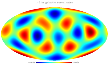
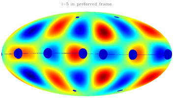
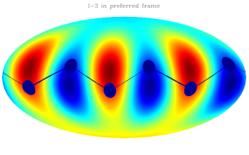
Figure 1: The $\ell=5$ multipole for a cleaned map in galactic coordinates (top) and aligned with $(b,l)\approx(50,-91)$ (middle.) We have superposed the multipole vectors, and the chain linking them. For comparison we plotted the $\ell=3$ multipole in its preferred frame.

It was suggested in teg that a possible statistic for anisotropy is

$$T_{\ell}=\max_{\bf n}\sum_{m}m^{2}|a_{\ell m}|^{2}$$ (2)

the average of $L_{z}^{2}$ maximized by an appropriate choice of $z$-axis; the outcome of this statistic is twofold: the value $T_{\ell}$ and the axis ${\bf n}_{\ell}$. This statistic favours high $m$s and so it works well in searches for planarity (i.e. $m=\pm\ell$). However the emergence of a preferred axis could come about from undue concentration of power in any $m$, a remark that is the main point of this letter.

We consider the alternative statistic:

$$r_{\ell}=\max_{m{\bf n}}\frac{C_{\ell m}}{(2\ell+1)C_{\ell}}$$ (3)

where $C_{\ell 0}=|a_{\ell 0}|^{2}$ and $C_{\ell m}=2|a_{\ell m}|^{2}$ for $m>0$ (notice that 2 modes contribute for $m\neq 0$). This statistic provides three basic quantities: the direction ${\bf n}_{\ell}$, the “shape” $m_{\ell}$, and the ratio $r_{\ell}$ of power absorbed by multipole $m_{\ell}$ in direction ${\bf n}_{\ell}$. The statistic is never ambiguous except for planar $\ell=2$ configurations, which may be interpreted as $m=2$ or $m=1$ modes with axis ${\bf n}_{2}$ rotated by $90^{\circ}$. As a convention we adopt the $(\ell=2,m=2)$ rendition for this configuration. In addition to the shape, direction, and strength of a given multipole we may also define inter-$\ell$ quantities, such as the angle between preferred axes for adjacent multipoles.

We have applied this method to a variety of maps: the cleaned and Wiener filtered maps of teg0 ; the internal linear combination maps erik3 (see also foregs ); the power equalized maps of biel . Taking cleaned and Wiener filtered maps, for $\ell=2,3$ our method promptly reproduces the results of teg ; copi : we find planar multipoles aligned with $(b,l)\approx(60,-100)$. For higher $\ell$ we find some surprising novelties. As an example, in Fig. 1 we plot $\ell=5$ (top two panels). Galactic coordinates obscure the fact that the multipole is very approximately a pure $m=3$ mode aligned with $(b,l)=(50,-91)$. This is revealed by our statistic and we have plotted the multipole when reoriented along its preferred axis. For comparison we plotted the $\ell=3$ mode aligned with its preferred axis.

A complete application of this scheme to higher multipoles is shown in Fig. 2. The multipole alignment found for $\ell=2,...,5$ does not extend to higher multipoles (even though there is a rough alignment of multipoles $\ell=6,...,11$ around a strip on the $b\approx 15$ latitude). However it is highly inconsistent with isotropy. We performed Monte Carlo simulations for Gaussian maps with the best fit power spectrum, subject to the WMAP noise and beam. We then considered the average value of all possible angles between vectors ${\mathbf{n}}_{\ell}$ for $\ell=2,...,5$. This is of the order of 20^∘ for the data. We find that only 5 out of 5000 simulations have an average value smaller than this. Thus we may reject isotropy on these scales at the 99.9% confidence level.

Other apparent anomalous features, however, are not as statistically significant as they appear. The ratios $r_{\ell}$, for instance, are completely consistent with Gaussianity, as the top panel of Fig.¬2 shows. For example, for $\ell=3$ we find that in the preferred frame 94% of the power is concentrated in the $m=3$ mode. This was seen in teg as anomalous, at the 93% confidence level. Indeed this is true if we insist upon planarity. If on the contrary we allow for anisotropy due to any kind of $m$-preference, then the majority of the simulations actually find a $m$ and ${\mathbf{n}}$ with a higher concentration of power in a single $m$; i.e. the observed $r_{\ell}$ is in fact low.

Likewise, the apparent preference for low $m$ multipoles (see Fig. 2) is not exceptional, once a more rigorous evaluation of the feature is obtained from Monte Carlo simulations (notice that the favoured $m$s are not uniformly distributed.)

Figure 2: A plot of $m$-preference results up to $\ell=20$. We seek the direction ${\mathbf{n}}_{\ell}$ (galactic coordinates in the bottom two plots) where a given $m$ (second plot from the top) receives the highest proportion of the power (with ratio $r_{\ell}$ plotted in the top panel). We have also plotted the Monte Carlo inferred variance for $r_{\ell}$. We plotted results for cleaned (solid), Wiener filtered (dash), and internal linear combination (dotted) maps as described in text.

However we do find another unusual feature with some statistical significance. Phase correlations have been proposed as a discriminator for localized non-Gaussian features in the sky phasescoles . In our formalism we may define $\ell$ azimuthal phases by examining the phases of the $a_{\ell m}$, for $m>0$, as measured in the preferred frame. Most important will be the phase of $a_{\ell m}$ for the $m$ that receives most of the power in this frame. This may be used to fix the $x$ and $y$ axes of the preferred frame; because there is an overall sign ambiguity between different $\ell$ and $m$ modes, phases separated by $\pi$ should be identified. Inter-$\ell$ features may then be studied using the full set of Euler angles relating the preferred Cartesian frames for different multipoles.

We find a very close alignment of the phases for the $\ell=3$ and $\ell=5$ modes. This should be blatant from Fig. 1, where we see that the longitudinal stripes of the two modes align very strongly. Comparison with Monte-Carlo simulations reveals that this feature is unusual to $94.5\%$. Other phases don’t correlate significantly.

This concludes the presentation of our basic results, which may be summarised as follows. The planar shape of the low $\ell$ multipoles is not statistically significant, once we allow the simulations to seek an axis maximizing power in a single, but general $m$. However the alignment of the preferred axis is indeed very significant and extends up to $\ell=5$. An additional azimuthal phase correlation brings to 99.995% the confidence level for rejecting Gaussianity and statistical isotropy.

We now examine the robustness of these results. Firstly they may be confirmed using an alternative technique: the Maxwell multipole vectors. These were first introduced by Maxwell maxwell over a century ago and have found a recent revival within the CMB community copi ; den1 ; us1 ; den2 ; weeks1 ; weeks2 ; lach . They encode the $2\ell$ degrees of freedom contained in a multipole beside the power spectrum (see us1 ; us2 ; den2 and ral for how these split into invariants and “eigenvectors”). Multipole vectors may potentially pick up $m$-preference since for pure $Y_{\ell m}$ configurations $\ell-m$ multipole vectors align with the preferred direction ${\mathbf{n}}$, with the remaining $m$ spreading at equal angles in the orthogonal plane – we call this a “handle and disc” structure, and it provides a more visual approach to detecting $m$-preference.

We consider these headless vectors in terms of pairs of points on the unit sphere. A handle is made through a clustering of points; a disc through a set of points tracing out an equator on the sphere. We look for these patterns by searching for the shortest routes between the points. The method does not provide a thorough search for m-preference, but can be used as a more visual tool to confirm and explore already noted features. In Fig. 1 we show how the method fares with $\ell=3$ where we find a single disk, and $\ell=5$ where we find a nearly exactly planar disk of 3 vectors and a handle of 2. More generally we confirm all the anomalous features described above. Where the two methods disagree there is no hint for $m$-preference.

How dependent are these results on the chosen data-set, i.e. on the concrete rendition of the large-scale anisotropies after the galactic emissions have been removed? We find that most publicly available maps agree on the features outlined above and only differ significantly beyond $\ell=12$. The cleaned and Wiener filtered maps of teg0 in fact agree almost exactly up to $\ell=12$ (see Fig. 2). Some features below $\ell=12$, however, are not as robust when we consider other maps. The quadrupole features, for instance, may be easily erased in the renditions of erik3 ; biel (see Fig. 2). The planarity of the $\ell=6$ mode is present in some renditions (and is detected by our statistic) but not in others. Thus we should regard these features as more fickle.

Figure 3: $m$-preference results up to $\ell=20$ for the V-band of galactic templates. We have included free-free (solid) syncroton (dot-dash) and dust (long-dash) maps; for reference we have reproduced results for the cleaned maps (dotted line).

This leaves us with the obvious question: what could cause the strange directionality of the large angle CMB fluctuations? Most obviously they could be due to systematic errors or galactic foregrounds. We subjected galactic templates foregs for synchrotron, free-free and dust emissions to this analysis (Fig. 3). Unsurprisingly we found a strong non-Gaussian signal; however nothing correlated with the direction or signal detected in the CMB maps. Specifically we found preference for $m=0$ modes for even $\ell$ and for $m=1$ for odd $\ell$. This preference is invariably found at $b=90$, i.e. with perfect alignment with the galaxy axis. The synchrotron and dust maps have very similar morphologies; the free-free emission is quite different and leads to more Gaussian $r_{\ell}$ ratios. None of this correlates with the features claimed for the CMB, even when the templates are mixed with a Gaussian component.

We also considered the simulated noise maps described in systs . These include all known systematic effects. We found that none of the available 110 simulated maps displayed any of the effects discussed in this paper.

Should the observed preferred axis be real our remarks may be crucial in identifying the culprit theory. We found that although there is a preferred direction for low multipoles (and to some extent a preferred Cartesian axis) this does not pick a specific $m$. Hence we don’t need a model favouring specific shapes (e.g. planarity); merely a model with a preferred axis. If the low $\ell$ fluctuations are due to the gravitational potential on the last scattering surface we can go further. The process may be described in terms of the potential Fourier modes $\Phi({\mathbf{k},\eta_{ls}})$; each of these modes is reflected in the CMB in a pattern with exact $m=0$ shape, with ${\mathbf{n}}$ aligned with ${\hat{\mathbf{k}}}$. One must superpose several such modes to obtain a given $\ell$, specifically:

$$a_{\ell m}=A\sum\Phi({\mathbf{k},\eta_{ls}})i^{\ell}j_{\ell}(k\Delta\eta_{ls})Y^{\star}_{\ell m}({\hat{\mathbf{k}}})$$ (4)

Superposing a large number of modes leads to no preferred direction or $m$ preference. Should the number of modes be limited to a lattice, though, a preferred shape and/or preferred axis will emerge. For a cubic lattice the low $\ell$ may become superpositions of mainly three modes $a_{\ell m}=A_{1}\delta_{m0}+A_{2}Y^{\star}_{\ell m}({\pi\over 2},0)+A_{3}Y^{\star}_{\ell m}({\pi\over 2},{\pi\over 2})$ and a solution in terms of $A_{i}$ may now be found for a given observed $m$-preference.

But it could also be that we live in a slab space, where there is a large number of modes in all but one direction. This will erase any preference for a specific $m$, while keeping the preferred direction. The choice between the two possibilities hinges crucially on the phase correlation found for $\ell=3$ and $\ell=5$, with the implication that there may be a preferred frame (rather than just a preferred axis). We find this feature the most tantalising aspect of our analysis.

Acknowledgements We thank Kris Gorski, Andrew Jaffe, João Medeiros and Max Tgemark for helpful comments. Some of the results in this paper were derived using the HEALPix package (healp ), and calculations were performed on COSMOS, the UK cosmology supercomputer facility.

References

- (1) A. de Oliveira-Costa et al., 2004, Phys. Rev, D69, 063516
- (2) Schwarz D. et al., Phys.Rev.Lett. 93: 221301, 2004.
- (3) J. Ralston and P. Jain, Int. J. Mod. Phys. D13, 1857, 2004.
- (4) Eriksen H.K. et al., 2004, Astrophys. J, 605, 14
- (5) Eriksen H.K. et al., 2004, astro-ph/0401276; astro-ph/0407271
- (6) H. Eriksen et al, ApJ, 612, 633, 2004 [astro-ph/0403098].
- (7) Hansen F.K., Banday A.J., Górski K.M.,2004,astro-ph/0404206
- (8) Land K., Magueijo J., 2004, astro-ph/0405519
- (9) Hansen F.K. et al., 2004, astro-ph/0402396
- (10) Vielva P. et al., 2003, astro-ph/0310273
- (11) Bennett C.L. et al., 2003, Astrophys. J. Suppl, 148, 1
- (12) J Weeks et al, Mon. Not. Roy. Astron. Soc. 352, 258, 2004.
- (13) B. Roukema et al, astro-ph/0402608.
- (14) N. Cornish et al, Phys. Rev. Lett. 92, 201302, 2004.
- (15) A. Berera, R. Buniy and T. Kephart, hep-th/0311223.
- (16) J. Moffat, astro-ph/0502110.
- (17) Ferreira P., Magueijo J., Górski K., 1998, Astrophys.J, 503, 1
- (18) A.J. Banday, S. Zaroubi, K.M. Gorski, astro-ph/9908070.
- (19) J. Magueijo, 2000, Astrophys. J. Lett, 528, 57
- (20) Magueijo J., Medeiros J., 2004, MNRAS 351, L1-4
- (21) Magueijo J., 1995, Phys. Lett, B342, 32. Erratum-ibid, B352, 499.
- (22) P. Ferreira and J. Magueijo, Phys. Rev. D56: 4578-4591, 1997.
- (23) M. Tegmark, A. de Oliveira-Costa and A. Hamilton, Phys.Rev. D68: 123523, 2003.
- (24) P. Bielewicz, K. Gorski and A. J. Banday, astro-ph/0405007.
- (25) Coles P. et al., 2003, astro-ph/0310252; P. Coles, astro-ph/0502088.
- (26) J. Maxwell, A treatise on Electricity and Magentism, Vol.1, Dover Publications, NY, 1954.
- (27) Copi C.J., Huterer D., Starkman G.D., Phys.Rev. D70, 043515, 2004.
- (28) M. R. Dennis, J. Phys. A 37 (2004) 9487-9500.
- (29) K. Land and J. Magueijo, astro-ph/0407081.
- (30) M. R. Dennis, math-ph/0410004.
- (31) G. Katz and J. Weeks, Phys.Rev. D70, 063527, 2004.
- (32) J. Weeks, astro-ph/0412231.
- (33) M. Lachieze-Rey, astro-ph/0409081.
- (34) K. Land and J. Magueijo, preprint.
- (35) Górski K.M., Hivon E., Wandelt B. 1998, astro-ph/9812350
- (36) C.L. Bennett, et al., 2003, ApJS, 148, 97.
- (37) G. Hinshaw, et al., 2003, ApJS, 148, 63.