HST/WFPC2 Color-magnitude Diagrams for Globular Clusters in M31

Abstract

We report new photometry for 10 globular clusters in M31, observed to a uniform depth of four orbits in F5555W(V) and F814W(I) using WFPC2 on board HST. Additionally we have reanalyzed HST archival data of comparable quality, for 2 more clusters. A special feature of our analysis is the extraordinary care taken to account for the effects of blended stellar images and required subtraction of contamination from the field stellar populations in M31 in which the clusters are embedded. We thus reach 1 mag fainter than the horizontal branch (HB) even in unfavorable cases. We also show that an apparent peculiar steep slope of the HB for those clusters with blue HB stars is actually due to blends between blue HB stars and red giants.

We present the color-magnitude diagrams (CMDs) and discuss their main features also in comparison with the properties of the Galactic globular clusters. This analysis is augmented with CMDs previously obtained and discussed by Fusi Pecci et al.  (1996) on 8 other M31 clusters. We report the following significant results:

1. The locus of the red giant branches give reliable photometric metallicity determinations which compare generally very well with ground-based integrated spectroscopic and photometric measures, as well as giving good reddening estimates.

2. The HB morphologies follow the same behavior with metallicity as the Galactic globular clusters, with indications that the 2nd-parameter effect can be present in some clusters of our sample. However, at [Fe/H]=$\sim-1.7$ we observe a number of clusters with red HB morphology such that the HB type versus [Fe/H] relationship is offset from the Milky Way and resembles that of the Fornax dwarf spheroidal galaxy. One explanation for the offset is that the most metal poor M31 globular clusters are younger than their Milky Way counterparts by 1-2 Gyr; further study is required.

3. The M_V(HB) versus [Fe/H] relationship has been re-determined and the slope ($\sim$0.20) is very similar to the values derived from RR Lyrae stars in the MW and the LMC. The zero-point of this relation (M_V = 0.51 at [Fe/H]=–1.5) is based on the assumed distance modulus (m–M)₀(M31)=24.47$\pm$0.03, and is consistent with the distance scale that places the LMC at (m–M)₀(LMC)=18.55.

1 Introduction

Among the Local Group galaxies, M31 has the largest population of globular clusters (GC) (460$\pm$70, see Barmby & Huchra 2001) and is the nearest analog of the Milky Way. Its distance from the Milky Way (MW), $\sim$780 kpc, is large enough so that the dispersion in distance modulus of the GC system can be considered to be small (50 kpc correspond to $\delta(M-m)\sim$ 0.15 mag), and hence the globulars are nearly at the same distance to us. Also, their almost stellar appearance (10 pc correspond to $\sim$ 2.6 arcsec) allows an easy study of their integrated properties from the ground.

On the other hand, M31 is also close enough that individual stars in GCs can be resolved and measured with HST (and with very large ground-based telescopes equipped with powerful adaptive optics systems. Therefore, good Color-Magnitude diagrams (CMDs) can be obtained, reaching well below the Horizontal Branch (HB), as was shown by the early HST surveys (Ajhar et al.  1996; Rich et al.  1996; Fusi Pecci et al.  1996 – hereafter Paper I, Holland et al. 1997; Jablonka et al. 2000; Stephens et al. 2001), and further confirmed by recent very deep observations using the Advanced Camera for Surveys on board HST (Brown et al.  2003, 2004a,b). In contrast to adaptive optics, HST not only avoids the vagaries of a spatially and temporally variable point spread function, but also gives imagery in the optical bandpasses which are most sensitive to metal line blanketing and have a vast heritage of prior studies.

While in many ways M31 is similar to the Milky Way, there are important differences. Brown et al.  find evidence for an age dispersion in the halo, with a metal rich population as young as 6-8 Gyr old. The halo itself appears to be dominated by stars acquired from the ingestion of other stellar systems, the signature of which is a halo of complex and irregular morphology, including a giant tidal stream (Ferguson et al.  2002). Finally, there has been a long standing question of chemical peculiarities in the M31 clusters, likely an enhancement of nitrogen (see Burstein et al.  2004, and Rich 2004).

The above mentioned issues make the detailed observations of the M31 GC system extremely valuable for very important comparisons with the analog systems in the MW and in external galaxies. The M31 GCs may be used as templates and a sort of bridge between fully resolved systems and totally unresolved ones in the study of stellar populations, with important implications for galaxy formation theories and cosmology.

From the observational evidence collected so far (see Perrett et al. 2002; Barmby 2003; Galleti et al. 2004, and references therein), the M31 GCs show all indications of being very similar to the MW globulars. Although no “direct” estimate of age, nor accurate metal abundances of individual star members, are available for any M31 GC except one (G312, see Brown et al.  2004b), most of them are presumably as old as, and slightly more metal-rich than the MW globulars. The two GC systems occupy similar loci in the “fundamental plane” (McLaughlin 2000) and seem to have similar M/L, structural parameters (Fusi Pecci et al.  1994; Djorgovski et al.  1997; Barmby et al.  2002; Djorgovski et al.  2003), and high incidence of strong X-ray sources (van Speybroeck et al.  1979; Bellazzini et al.  1995; Di Stefano et al.  2002, Trudolyubov & Priedhorsky 2004).

However, as previously mentioned, the globular cluster system exhibits noteworthy contrasts with that of the Milky Way:

a) By comparing integrated GC colors with stellar population models, Barmby et al.  (2001) concluded that the metal-rich GCs in M31 are younger (by 4-8 Gyr) than the metal-poor ones. A similar interpretation was suggested to explain the stronger H$\beta$ lines observed in metal-rich M31 GCs compared to Galactic globulars (Burstein et al.  1984), but Peterson et al.  (2003) proposed an alternative explanation based on the presence of old blue HB stars (see also Fusi Pecci et al.  2004).

b) The metallicity distribution of M31 GCs is clearly bimodal (Barmby et al.  2000) and there are indications (Huchra et al. 1991; Perrett et al.  2002) for a systematic difference in kinematics and spatial distribution between the two metallicity groups, somehow supporting possible differences in the formation process and age (Ashman & Zepf 1998; Saito & Iye 2000). In particular, Morrison et al.  (2004) claim that there is a subsystem of GCs in M31 with thin disk kinematics, whereas no GC is known to be associated with the Galactic thin disk.

c) There are indications for possible variations of the GC Luminosity Function (Barmby et al.  2001) and average structural parameters (Djorgovski et al.  1997, 2003; van den Bergh 2000; Barmby et al.  2002) with galactocentric distance and metallicity, that might be ascribed to differences in age, destruction/survival/capture rate, etc.

d) There is clear evidence for the existence of streams and overdensities associated with metallicity variations across the whole body of M31 (Ibata et al.  2001; Ferguson et al.  2002), possibly related to interactions with close companions (Bellazzini et al.  2001; Bekki et al.  2002; Choi et al.  2002). On analogy to what has occurred between the Sagittarius dSph and the MW (Ibata et al.  1994), it may be conceivable that also a fraction of the M31 GCs was captured and differs in some property (age? chemical composition? kinematics?) from the main body of “native” clusters. In this respect it may be worth noting that M32 does not appear to have any (residual) GC system (van den Bergh 2003).

The above issues can be studied using different and complementary approaches. For example, one could observe the integrated light of GCs in specific bands or indexes (far UV, H$\beta$, IR, etc.) sensitive to age, or metallicity, or peculiar HB-morphology (or, more probably, a hard-to-disentagle mixture of them). Or, one could study some very special stellar populations, e.g. the variables (see the detection of several possible RR Lyrae candidates in four M31 GCs by Clementini et al.  2001), or the X-ray sources. However, the past forty years of research on Galactic GCs taught us that one can hardly hope to reach any firm and unambiguous conclusion whithout having the CMDs and (possibly) the spectra of individual stars.

If we aim to assay the age of the cluster system, it is possible to do so directly by the measurement of main sequence photometry. In M31, a 12 Gyr old population has a main sequence turnoff (TO) at V$\geq$28.5 and photometry must reach 1-2 mag fainter for a precise age measurement for the oldest stars. This has been accomplished in one field in M31, by investing 120 orbits of imaging with HST+ACS (Brown et al.  2003, 2004a). Due to extreme crowding, a somewhat less stringent age constraint was determined for the cluster G312 (Brown et al.  2004b) in the same deep ACS field. For the foreseeable future, such a campaign will be practical for a very small number of fields. Combining spectroscopy and SEDs offers (in principle) another approach to constraining the age. This approach is enjoying an increasing level of success. However, the measurement of CMDs to below the horizontal branch gives an additional age constraint and a powerful means of comparing the M31 clusters with other cluster populations. Knowledge of the actual CMDs also improves the accuracy of spectroscopic and SED based methods.

As mentioned above, all we presently know about the GCs in M31 rests on colors and metallicities from integrated ground-based photometric and spectroscopic observations (Barmby & Huchra 2001; Perrett et al. 2002; Galleti et al. 2004, and references therein), and on the CMDs of the few clusters previously observed with HST (Ajhar et al. 1996; Rich et al. 1996; Fusi Pecci et al. 1994, 1996; Holland et al. 1997; Jablonka et al. 2000; Stephens et al. 2001).

With the HST-WFPC2 observations (GO program 6671, P.I. Rich) we present here we have more than doubled the number of clusters observed with HST. Preliminary results obtained from these data were presented by Corsi et al.  (2000) and Rich et al.  (2001). The present paper reports the final results on these 10 additional GCs in M31. In the following discussion we add two more clusters using archive WFPC2 data that were obtained in very similar conditions (GO program 5906, P.I. Holland).

In Sect. 2 we present a description of the data, and the data reduction, field subtraction and calibration procedures. The presentation and analysis of the results, in Sect. 3, include some discussion on the overall properties of the CMDs we have obtained (considering also the CMDs of the 8 M31 GCs described in Paper I) and a general comparison with typical Galactic globulars. In particular, we discuss the Red Giant Branch (RGB) and Horizontal Branch (HB) location and morphology, and the estimate of parameters such as (photometric) metallicity, reddening, HB-type, HB-luminosity level, and M31 distance. A summary and conclusions can be found in Sect. 4.

2 The data

2.1 Observations

Our target GCs were selected from the brightest (i.e. most populous) objects, over a wide range of radial distances and metallicities, taking into account also the clusters that had been observed before with HST (Rich et al.  1996; Ajhar et al., 1996; Fusi Pecci et al., 1996; Holland et al., 1997). We have deliberately avoided the innermost and reddest clusters for which the crowding is so severe as to compromise photometry in the visible bands (see Jablonka et al.  2000; Stephens et al.  2001).

Ten clusters were observed under program GO-6671 (P.I.: Rich), using the WFPC2 on board HST, and the filters F555W (V; 4 images of 1200, 1300, 1400, 1400 sec on each cluster) and F814W (I; 4 images of 1300,1300,1400,1400 sec on each cluster). The clusters were all centered on the PC frame that provided the best spatial resolution, except G91 that fell in the WF3 frame while the PC was pointed on G87. For two additional clusters, G302 and G312, that were observed with the same HST+WFPC2 setup in the program GO–5906 (P.I.: Holland), we retrieved the data from the HST archive. The total exposure times are 4320 sec (V band) and 4060 sec (I band), so the data are comparable with ours.

In Table 1 we give the journal of observations for these clusters, as well as some basic parameters. Their images in the I band are shown in Fig. 1.

2.2 Data reduction

The HST frames were reduced using the ROMAFOT package (Buonanno et al.  1983) which is optimized for accurate photometry in crowded fields, and has been repeatedly updated to deal with HST+WFPC2 frames. In particular, the PSF is modeled by a Moffat (1969) function in the central part of the profile plus a numerical experimental map of the residuals in the wings. The optimal PSF is determined from the analysis of the brightest uncrowded stars independently in both sets of V and I co-added frames.

The individual frames for each field of view were first aligned and stacked so as to identify and remove blemishes and cosmic ray hits; this procedure also made it possible to detect and identify the accurate positions of all point sources including the faintest ones. Finally, the photometric reduction procedure was performed on the individual frames and the instrumental magnitudes of each star were averaged with appropriate weights. This procedure allowed us to achieve a better photometric accuracy than performing photometric measures on the stacked frames. No corrections for non-linearity effects were applied, because it was verified that they were not necessary.

Individual stars were measured in radial annuli whose distances from the respective cluster centers depend on the intrinsic structural properties of the GCs and on the crowding conditions. We report in Table 2 for each observed cluster the annulus where photometry was done, and the percentage of sampled light/population over the total ($L_{sam}/L_{tot}$). The value of $L_{sam}/L_{tot}$ has been computed by integrating the light in the annulus directly from the cluster profile as obtained in the study of the structural parameters (Parmeggiani et al.  2005 – Paper III, in preparation - Djorgovski et al.  2003). More internal areas were too crowded for individual stellar photometry, and more external areas were dominated by field population.

The above procedure assumes that the clusters are projected spherical. This may be incorrect in some cases, as shown, for example, by Lupton (1989) and Staneva et al. (1996) using ground-based data, and confirmed by Barmby et al. (2002) and Parmeggiani et al. (2005) using HST data. On the basis of these HST data, we estimate an average ellipticity of 0.11 for all clusters except two (G1 and G319) for which the ellipticity is about 0.2. Therefore, the error we make on the $L_{sam}/L_{tot}$ ratio by assuming a spherical rather than elliptical light distribution is smaller than 10$\%$ in all cases, and is irrelevant for the present analysis.

2.3 Calibration and photometric accuracy

The calibration to standard V and I magnitudes was performed according to the procedure outlined in Dolphin (2000) (updated as described in the web site). ¿From this procedure, that accounts for both the charge transfer efficiency and the variations of the effective pixel area across the WFPC2, we have obtained the final calibrated magnitudes in the Johnson photometric system.

The final internal photometric errors are $\sim 0.02$ mag in (V, I) and $\sim 0.03$ mag in (V-I) for V $<$ 24.0, and $\sim 0.06$ mag in (V, I) and $\sim 0.08$ mag in (V-I) for V $>$ 25.5. Therefore, at the level of the HB (V $\sim$ 25) the photometric errors are typically $\sigma_{(V,I)}\sim$ 0.05 mag and $\sigma_{(V-I)}\sim$ 0.06 mag.

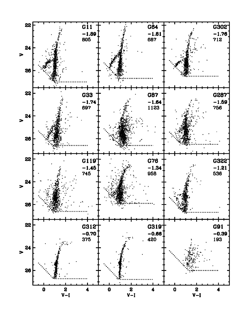
Figure 2: Observed CMDs for the 12 M31 GCs analysed in the present study. Each cluster is labelled with its name, metallicity, and number of stars displayed (i.e. all the stars detected and measured within the annuli listed in Table 2). The dotted lines represent the limiting magnitude cutoffs of the photometry.

The limiting magnitudes of our photometry, defined as 5-sigma detections, run from V $\sim$ 26.2 and I $\sim$ 25.5 in the worst crowding case (i.e. G76) to V $\sim$ 27.2 and I $\sim$ 26.3 in the best case (i.e. G11). The limiting magnitude cutoffs are shown as dotted lines in the CMDs presented in Fig. 2. These CMDs contain all the stars that were detected and measured in each cluster within the annuli specified in Table 2.

2.4 Field subtraction

For each globular cluster the surrounding field was studied using the corresponding WFC frames. These were reduced with the photometric package DoPhot, which runs much faster than ROMAFOT and equally accurate where the crowding is not too severe. The calibrations are compatible, within the observational errors, with those obtained for the globular clusters using ROMAFOT on the PC frames. The detailed analysis and results on the surrounding fields are presented in a separate paper (Bellazzini et al.  2003).

Our initial approach used the outermost annulus in each PC frame to define the field population for statistical subtraction, but the field was so small as to lack enough stars for a meaningful background sample. Therefore the use of the more external and much larger WFC fields seemed preferable as it provided a better statistical base for field subtraction, once verified that the different reduction packages applied to the PC (i.e. globular clusters) and WFC (i.e. fields) frames yield comparable results. The statistical field subtraction was performed using the algorithm and the procedure developed and described by Bellazzini et al.  (1999b, their Sect. 3) which is very similar to that adopted by Mighell et al.  (1996). As widely discussed by Bellazzini et al.  (1999a), any procedure aiming at statistical decontamination suffers of some degree of uncertainty. The effects of decontamination on the various parts of the CMD are hard to evaluate in detail, because of the complex effects of crowding, completeness variations and background determination. In addition, effects due to the possible existence of tidal tails can be present, as discussed, for example, by Grillmair et al. (1996), Holland et al. (1997), and Barmby et al. (2002). However, as noted by Meylan et al. (2001), a proper consideration of the tails would need to reach stars a few magnitudes fainter than the turnoff to have a statistically significant sample of such escaping stars. This is not our case, because of the brighter limiting magnitudes of our photometry.

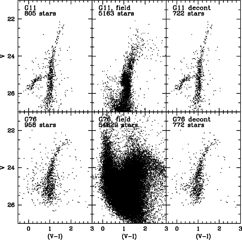
Figure 3: Examples of statistical field subtraction: CMD of G76 and G11, before (left) and after (right) field subtraction. The middle panel shows the CMD of the corresponding field, defined over a much larger WFC area.

As an example, we show in Fig. 3 the CMDs of two clusters, G76 and G11, that represent the worst and best cases of crowding conditions, respectively. For each we show the CMD of the globular cluster before and after field subtraction, and the CMD of the corresponding subtracted field. As expected, when the crowding is low the field contribution is nearly irrelevant, and when the crowding is high the subtraction of the field may have significant effects (see Sect. 3.2.1).

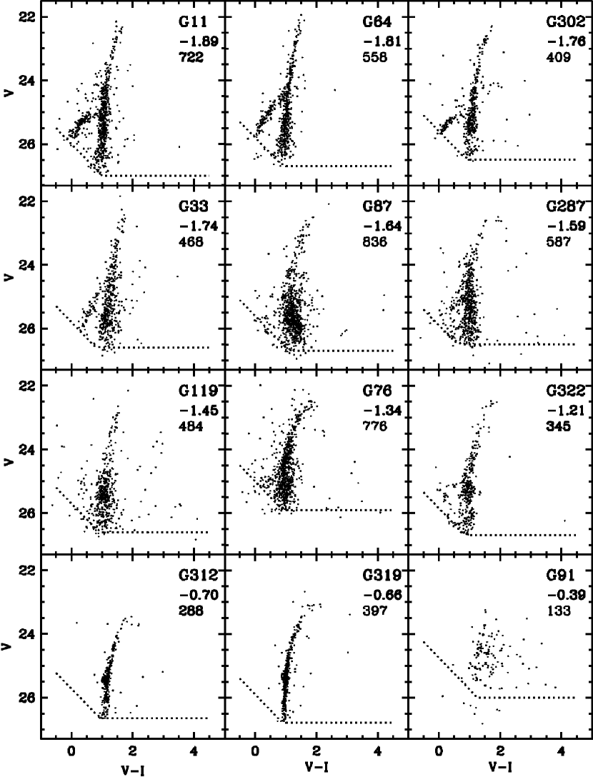
Figure 4: As in Fig. 2, where the CMDs have been cleaned of field contamination. The number of stars displayed in each panel represents those that are left after field subtraction.

Since in the present analysis we aim at defining ridge lines and average properties of the various branches of the CMDs, the statistical decontamination helps in “cleaning” these features from the field stellar contribution, makes their detection easier and highlights the information there contained. Therefore we have applied the statistical field subtraction to all our clusters according to the procedure described above. We list in Table 2 the total number of measured stars in each CMD and the number of stars left after statistical field subtraction, and we show the corresponding field-subtracted CMDs in Fig. 4.

2.5 Photometric blends

An inspection of Fig. 4 reveals that, in several clusters, the HBs appear unusually steep and heavily populated also on the red side of the HB, quite at odds with the shape one would normally expect by comparison with Galactic GC of similar metallicity. This is especially striking in the most metal-poor clusters with normally blue HB morphologies, and the stars populating the steep red HB branch do not correspond to any “classic” evolutionary phase. The most plausible explanation is that these unusual features are the result of photometric blends. To support this suggestion we take G64 as an example, and show it in detail in Fig. 5. In the top left panel we show the CMD of the entire stellar sample we have measured, after field decontamination. The HB, with unquestionably blue morphology in agreement with the cluster metallicity, seems to extend in a rather steep sequence to the bright and red side, at V$<$25 and 0.4 $<(V-I)<$ 1.0. In the other panels we show the CMDs of the stars in progressively more external areas of the cluster, and we see that this feature becomes less significant and eventually disappears at a radial distance of about 3.2 arcsec (i.e. 70 px). This evidence strongly suggests that this feature is due to photometric blends and not to real stars.

To test this hypothesis we have performed a simulation based on the ”artificial stars” method. Since the degree of crowding is highly variable with radial distance, we have considered three rings at 45$<r<$60 px, 60$<r<$80 px and $r>$80 px, and determined the completeness curve for each of them. Fig. 6 reports the results of this test in G64. As can be seen, the degree of completeness is a strong function of distance from the cluster center, as expected. From the plot one can draw two important indications: a) the completeness drops below 90% at V$\sim 23.8$ (i.e. well above the HB level) in the innermost bin, at V$\sim 24.8$ (i.e. just above the HB level) in the intermediate bin, and at V$>25.8$ (i.e. fainter than the HB) in the outer ring; b) the fraction of recovered stars in the inner rings, and in particular in the intermediate one, is higher than 100$\%$. We interpret this fact as due to blending effects which produce more luminous stars at the expense of the fainter ones, thus “drifting” part of the fainter stellar population into an artificial brighter stellar population in the more internal (crowded) rings.

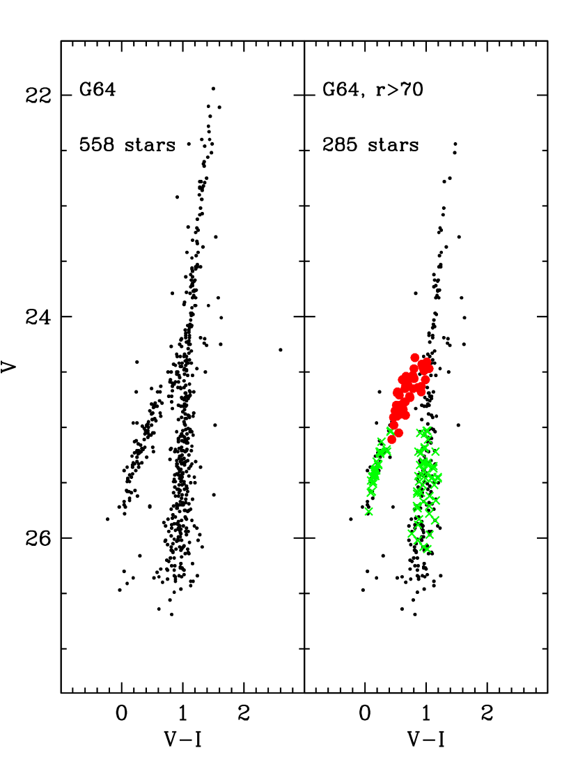
Figure 7: CMDs for G64: the left panel shows the entire CMD after the subtraction of the field; in the right panel we have superposed to a more external CMD (r$>$70 px) several ’fake’ simulated stars (shown as red dots) resulting from the photometric blend of HB and RGB stars (shown as green crosses).

As well known, if the co-added stars have different luminosities the luminosity and color of the blend are nearly the same as those of the brighter component; if the two stars have similar colors one would observe just a brightening (up to 0.75 mag for equal components); however, if the two stars have similar brightness and different colors (blue and red), the resulting blend is brighter and with an intermediate color. This is exactly what has occurred with the bright red stars we are observing on the red HB. To confirm this explanation, we show in Fig. 7 how the simulated combination of an HB star fainter than V=25 and bluer than (V-I)=0.4 with a red giant star of similar luminosity and (V-I)$\sim$1 produces exactly this type of feature. Both blue HB and red giant stars are abundant in metal-poor clusters, and the extremely high density conditions in the innermost areas favor the occurrence of photometric blends.

Therefore, we have repeated for all clusters the inspection of the CMDs over progressively more external areas to identify spurious features due to blends, if any, and the radial distance at which these features become irrelevant. In the last two columns of Table 2 we list these values of radial distance, and the number of stars left in each CMD after subtracting the likely blends. In the following analysis we use CMDs that are decontaminated from field and blend contributions, for a better definition of the CMD intrinsic characteristics.

3 The CMDs: Results and Analysis of the Main Branches

We show in Fig. 4 the CMDs for the 12 globular clusters considered in the present study, after decontamination from the field contributions.

We note that the CMD morphologies are generally consistent with the metallicity content in much the same way as in Galactic GCs: (a) the slope of the red giant branch decreases with increasing metallicity, and (b) the bulk of the HB population is progressively shifted from the red in the metal-rich objects towards the blue in the metal-poorer ones.

This indicates that the M31 GCs included in the present sample are on average similar to those of the MW. It is worth noting that if we had a large enough sample (say 50-60) of CMDs of this quality for the M31 GCs, our knowledge of the M31 GC system would be comparable to what we knew about the MW GCs in the early 1970s. This level of knowledge could easily be achieved with HST.

Relying on the evidence of the substantial similarity between the two GC systems and using our knowledge of Galactic GC as reliable templates, the morphology and characteristics of the two main features of these CMDs, namely the RGB and the HB, can be inspected and used to derive information on a number of parameters, that are described in detail in the following sections. However, we first consider the reddening which has major impact on the determination of parameters such as metallicity and distance, as discussed later.

3.1 Individual reddenings from the literature

The extinction in the direction of M31 is due to dust that can reside either in our Galaxy or within M31. A reliable estimate of average reddening due to Galactic material can be obtained from reddening maps (Burstein & Heiles 1982; Schlegel et al. 1998), whereas no estimates are available of the internal reddening, and this is one of the major sources of uncertainty in the study of the stellar populations in M31 (see Barmby et al.  2000).

The Galactic reddening in the direction of M31 was estimated by many authors: van den Bergh (1969) found E(B-V)=0.08, McClure & Racine (1969) give 0.11, Frogel et al.  (1980) 0.08, Crampton et al.  (1985) 0.10, Jablonka et al.  (1992) 0.04. The maps of Schlegel et al.  (1998) yield a value of about E(B-V)=0.06 in the direction of M31.

The reddening of individual GCs in M31 has been estimated by several ways, all of them quite uncertain. Vetesnik (1962) derived color excesses for 257 candidate GCs by assuming an average true color for 36 GCs located well outside the body of M31, which implied that these clusters were only affected by the foreground Galactic extinction. Later, many authors adopted the simplified assumption of a single intrinsic color for all GCs in M31. Frogel et al.  (1980) estimated the individual reddening for 35 GCs using the reddening-free parameter Q_K from unpublished spectroscopic data taken by L. Searle. Crampton et al.  (1985), using their spectroscopic slope parameter S, derived a relationship between (B-V)₀ and S and computed the intrinsic colors and the color excesses for about 40 candidates in their sample. Barmby et al.  (2000) determined the individual reddenings for 314 GCs candidates by assuming that both the extinction law and the GC intrinsic colors are the same as in the MW and using correlations between optical and infrared colors and metallicity, and by defining various “reddening-free” parameters.

We list in Table 3 the individual values of reddening available in the literature and their sources. Some of these reddenings appear as negative values, just as a result of the reddening determination procedure. These values are obviously unphysical, and we have replaced them with the value 0.06 which represents the Galactic reddening in the direction of M31 according to Schlegel et al. (1998) maps, and hence a lower limit for the M31 reddening. The values we eventually adopted for use in the following sections (see column 12) are the unweighted average of the figures reported in Table 3, with the following criteria: i) the estimates by Vetesnik (1962) and van den Bergh (1969) were not used because their accuracy is rather poor; ii) the double estimates obtained by using two sets of (B–V) colors and the relations from Crampton et al.  (1985) (columns 8 and 9) and from Barmby et al.  (2000) (columns 10 and 11) were considered only once each, taking their respective mean values; and iii) no mean reddening value was allowed to be smaller than 0.06 mag; when that happened (i.e. G219 and Bo468), the value 0.06 was adopted instead.

Some individual estimates are more reliable than others, varying from object to object, and it is difficult to assess precisely the error to associate to the final adopted figures. By comparing the various sets of data from the different quoted sources for the low-reddened GCs, a typical error for the adopted E(B-V) values should be about 0.04 mag, but it can well be larger for some objects and smaller for others. In Table 3 we list also the dispersion ($\sigma$) values of our adopted mean reddening estimates, just to show how the individual estimates can vary.

As discussed in Sect. 3.2.2, such an uncertainty in the knowledge of the individual reddenings may have quite a significant impact on the determination of both metallicity and relative distances based on the comparison of the CMDs.

3.2 The Red Giant Branch (RGB)

The color and morphology of the RGB are sensitive to metallicity, and its luminosity function (if sufficiently populous and complete) gives a constraint on the cluster distance and stellar evolution. The present data do not permit us to use either the RGB tip for distance determination, or the RGB bump for a metallicity constraint.

3.2.1 The RGB ridge lines

At the bright end, cluster ridge lines suffer from the small sample size while larger photometric errors offset the larger numbers of stars on the subgiant branch. For each cluster the RGB has been fitted by a second- or third-order polynomial law of the form (V–I)=$f$(V). After each iteration, stars deviating more than 2$\sigma$ in color from the best-fitting ridge line were rejected and the fitting procedure was repeated until a stable solution was reached.

We can measure the RGB ridge line to $\pm$0.02 mag (color), except for the bright end of the RGB in sparsely populated CMDs. We have compared the ridge lines derived from the decontaminated (i.e. field and blend subtracted) population to the ridge lines derived from the observed population in two annuli at different radial distances. We note that the decontaminated ridge lines coincide with the observed ridge lines in the inner annulus, and are slightly bluer (by $\sim$ 0.02 mag) than the observed ridge lines in the outer annulus. This effect was noticed also in Paper I. From the present results this appears to be due to field contamination, that has a stronger effect on more external cluster areas and was not taken into account in Paper I, and not to a real color gradient across the clusters. Incidentally, the effect of photometric blends is not very important along the RGB: whereas the blend of a blue and a red star would produce the feature discussed in Sect. 2.5, which stands out clearly in the CMD, the blend of two red stars would produce a brighter red star and contribute to increase only slightly the scatter in color, with no detectable distortion of the RGB within the errors.

We list in Table 4 the ridge lines we have derived for all the clusters considered in this study except G91 for which a reliable ridge line could not be defined. A similar table was presented for the 8 clusters studied in Paper I (see their Table 2), and since the procedure for the ridge line determination is the same, the two data sets are sufficiently homogeneous and can be used jointly in the following considerations.

3.2.2 Metallicities

In sufficiently old clusters (t $>$ 10 Gyr) the shape and color of the RGBs depend most strongly on metallicity and reddening (for a given treatment of opacity, convection etc. this is reproduced also by the models). Therefore, in principle, if either of these parameters is known independently, reliable estimates of the other parameter can be obtained using the calibrations based on Galactic GCs, assuming that the two GC systems are similar.

In practice, however, besides the uncertainty in tracing the RGB ridge lines, the procedure is further complicated by obvious issues (photometric calibration) as well as other factors (clusters dispersed over a 20 kpc radius would have up to 0.06 mag random distance uncertainty). Further issues are the calibration of color vs [Fe/H] and, finally, dependence on cluster composition. Our data also are not good enough to permit us to use the method of Sarajedini (1994) which would simultaneously determine E(V-I) and [Fe/H].

A metallicity estimate would come either from some reddening free parameter calibrated in terms of [Fe/H] or by assuming a value for the reddening and comparing the dereddened cluster RGB with a grid of calibrated ridge lines.

We have decided to apply the first procedure using the $S$ parameter defined by Saviane et al.  (2000), and to compare the results with the RGB interpolation. We also anticipate that having adopted as reference grid the ridge lines of Galactic GCs with known reddenings, metallicities and distance moduli, we apply an iterative procedure to the whole CMD (i.e. including both the RGB and HB) which would yield the “best-fitting morphological” solution for reddening, metallicity and relative distance modulus, without making any a priori assumption. This latter approach is somewhat arbitrary but has the advantage of adding constraints from the HB morphology.

The metallicity from the RGB slope

Several indexes related to metallicity can be defined, based on the morphology of the RGB (see Ferraro et al.  1999; Saviane et al.  2000). Of all these parameters only one, the so-called $S$ parameter, is reddening-free: it is defined as the slope of the line connecting two points on the RGB, the first one at the level of the HB, and the second one 2 mag brighter than the HB. Being a slope, this quantity is naturally independent of both reddening and distance, depending only on the shape of the RGB and hence, metallicity.

Originally defined by Hartwick (1968) in the (B, B–V) plane, the $S$ parameter has been recently redefined and recalibrated in the (V, B–V) plane by Ferraro et al.  (1999) using high quality CMDs of 52 Galactic GCs collected from different sources, and in the (V, V–I) plane by Saviane et al.  (2000) using the homogenous sample of V,I CMDs for 31 Galactic GCs observed by Rosenberg et al (1999). These parameters are identified as $S_{2.0}$ and $S$, respectively. Ferraro et al.  (1999) provide relations (see their Table 4) between their $S_{2.0}$ parameter and both [Fe/H] (in the Carretta and Gratton 1997 – CG97 metallicity scale) and total [M/H] metallicity, and the rms error of their fits is $\sigma$=0.18 dex. Saviane et al.  (2000) provide relations (see their Table 6) between their $S$ parameter and [Fe/H] in both CG97 and Zinn and West (1984 – ZW84) metallicity scales, and the rms error of their fits is $\sigma$=0.12-0.13 dex.

We have measured the $S$ parameter for all the M31 GCs in our present sample, except G91 for which neither the RGB ridge line nor the HB magnitude level can be reliably defined. In addition, we have derived the $S$ parameter for the 6 clusters in Paper I with V and I data, and the $S_{2.0}$ parameter for the 2 clusters (G280 and G351) with B and V data. For the magnitude level of the HB, that enters in the definition of $S$, we have used the values described in Sect 3.3.2 and listed in Table 8, that have an average rms error of $\pm$0.1 mag. Taking into account this uncertainty, the average error $\Delta(V-I)=\pm$0.02 in the definition of the RGB ridge lines (see Sect. 3.2.1), and the rms error 0.12 dex of the calibration fit (Saviane et al.  2000), we estimate that the average rms error of our metallicity determinations using the $S$ parameter varies from $\Delta[Fe/H]\sim\pm$0.28 dex for the most metal-poor clusters (e.g. G11), to $\sim\pm$0.24 dex for intermediate metallicity clusters (e.g. G287), to $\sim\pm$0.15 dex for the most metal-rich ones (e.g. G319). Table 5 reports the values of $S$ and $S_{2.0}$ for the entire cluster sample, and the values of metallicities we have derived using the Saviane et al.  (2000) and Ferraro et al.  (1999) relations, as appropriate.

The metallicity from comparison of the RGB with template ridge lines

As was done in Paper I for 8 GCs and in Bellazzini et al.  (2003) for 16 fields, metallicities can be estimated by comparing directly the target RGBs with a reference grid of Galactic GC (GGC) fiducials of known metallicity, after correcting for the respective reddenings and distances. The accuracy of this procedure depends mostly on how finely the metallicity range is sampled, as well as on the accurate knowledge of the reference grid relevant parameters (i.e. reddening and distance).

In order to check the results derived above with the $S$-parameter, we have applied to our M31 GCs the same interpolating procedure used by Bellazzini et al.  (2003). The reference grid of GGCs and their parameters are listed in Table 6. The V and I photometric data used to derive the HB and RGB ridge lines of the reference clusters have been taken from Rosenberg et al. (2000a,b) and Guarnieri et al. (1998) except for the clusters G280 and G351, that have HST-FOC B and V data. For them, the template HB and RGB ridge lines were derived from the B,V database of GGCs collected by Piotto et al.  (2002).

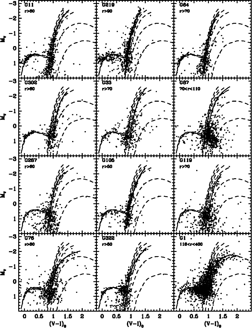
Figure 8: RGB ridge lines of our GCs (shown as solid lines), plotted individually along with the grid of GGC RGB templates (shown as dashed lines). The (M_V/(V-I)₀ templates are for: NGC6553, 47 Tuc, M5, M3, NGC6397 and M15 (see Table 6).

We show in Fig. 8 and 9 the CMDs of our M31 GCs, plotted individually along with the grid of HB and RGB template ridge lines, for comparison. For the M31 clusters we used the CMDs that had been previously cleaned of field and blend contamination, and corrected them for reddening and absorption using the relations E(V–I)=1.375E(B–V), A_V=3.1E(B–V) and A_I=1.94E(B–V) (Schlegel et al. 1998) and the adopted reddening values listed in Table 3 (column 12) as initial input values. Then each target cluster CMD is shifted in magnitude until reaching a satisfactory match with both HB and RGB ridge lines of a template CMD, or of an “interpolated” solution between two bracketing templates. The metallicity of the template, or the intermediate value between the bracketing templates if interpolation is needed, is the adopted metallicity. The accuracy of these estimates is typically half the interval of the bracketing templates, about $\pm$0.15-0.20 dex at the most metal-poor end of the metallicity range, and $\leq$0.1 dex at the metal-rich end. These values are listed in Table 5 col. 6 (labelled $Ridge$).

This procedure also yields an estimate of distance via the magnitude shift that needs to be applied in order to match the target CMDs with the templates. In some cases an additional shift in magnitude with respect to the average distance assumed for M31 is necessary to achieve an acceptable match. If no color shift is involved as well, this can only be interpreted as a distance effect, indicating that the cluster distance is larger or smaller than the distance we have adopted for M31, i.e. (m–M)₀=24.47$\pm$0.03 (weighted mean of the most recent determinations from Holland 1998; Stanek & Garnavich 1998; Freedman et al.  2001; Durrell et al.  2001; Joshi et al.  2003; Brown et al.  2004a; McConnachie et al.  2004). We remind the reader that a dispersion of $\pm$0.06 mag in the distance moduli can well be intrinsic if our clusters are located on a spheroidal distribution with $r\sim$20 kpc. We have listed these distance moduli in Table 7 along with the corresponding values of (adopted) reddening and (derived) metallicity (columns 3-5), for the sake of convenience when we discuss the issue of distance estimates (Sect. 3.3.2).

To get the largest possible sample, we apply this procedure to all available M31 GCs including those of Paper I. As shown in Fig. 8 and 9 we get a satisfactory match in most cases, but it is also evident that some CMDS (e.g. G322) require an additional color shift before they match the Galactic fiducials. This kind of problem leads us to consider one final method below.

An alternative experiment: a global “best morphological match” with the reference grid

Before comparing our photometric metallicities with other approaches, we compare M31 to MW clusters using yet a different method, required by the few CMDs which fail the aforementioned grid because they require a color shift. The aim is search for the best match of both the RGB and HB while leaving distance and reddening as free parameters.

The values of metallicity thus derived are listed in Table 5, where we collect all available estimates of metallicity for our clusters. The set of values for reddening, metallicity and distance that yield the best match are reported in Table 7, columns 6-8.

3.2.3 Final considerations on reddening and metallicity

Considering the results obtained in the previous sections, it is now possible to discuss these parameters in some more detail.

Reddening
A comparison of the figures reported for each cluster in Table 7 (columns 3 and 6) shows the difference between the adopted value derived in Sect. 3.1 as the mean of the available estimates in the literature, and the value obtained by the “best 3-parameter match” of the whole CMD. The two values agree generally within the estimated error of $\pm$0.04 mag except for a few clusters. The clusters for which $\Delta E(B-V)>$ 0.04 mag are G33, G108, G280, G302, G319 and G322.

Since we do not have any external strong constraint on metallicity and distance modulus which might clarify the choice, we keep as the most probable values of reddening those adopted in Sect. 3.1 and listed in Table 3, column 12 (reported also in Table 7, column 3), recalling however the caution implied by the worse global fit.

Metallicity
In Table 5 we list all the available independent estimates of metallicity, for ease of comparison. In addition to those obtained from the $S$-parameter (col.s 4 and 5) and from the two CMD-fits (col.s 6 and 7), there are three further determinations, two of which based on spectra and one on optical and IR photometry.

The spectroscopic estimates are from calibrations applied to spectral line indices in the cluster integrated spectra. In particular we report the data from Huchra et al.  (1991), collected by Barmby et al.  (2000) and Perrett et al. (2002).

Photometric estimates use integrated (V–K) colors calibrated in terms of [Fe/H] in the ZW metallicity scale by Bonoli et al.  (1987). The photometric estimates require the knowledge of the individual reddenings, which were adopted by Bonoli et al.  (1987) as E(B–V)=0.10 for all the considered clusters except G33 and G64, for which 0.22 and 0.17 were used, respectively.

These different techniques give a range in accuracy and reliability. For the old clusters the metallicities derived from the spectra are probably the most reliable in spite of the uncertainties and ambiguities related to the definition, meaning and calibration of the spectroscopic indexes used for these determinations (Burstein et al.  2004 and references therein).

On the other hand, the results from the ridge line fitting method are mostly qualitative and generally give only a rough consistency check.

The $S$-parameter and the integrated IR photometry do not measure metallicity directly, but rely on some type of calibration which may introduce additional uncertainty. However, they are quantitative and relatively accurate methods and should yield quite reliable results. Incidentally, we note that the $S$-method depends only on the RGB morphology, as well as the integrated IR photometry that is obviously mostly sensitive to the RGB stellar population, whereas spectroscopic metallicities are based on integrated visual spectra that may be affected by other types of stellar populations than the RGB, if sufficiently abundant or luminous.

We are pleased that for most clusters, the metallicity estimates we obtain from the RGBs, both via the $S$ paramter and from direct comparison with RGB templates agree well with the other estimates.

From the above methods we derive mean values of metallicity for our clusters using a straight unweighted average of the values obtained from the $S$ parameter, RGB ridge line fit, spectroscopic estimates, and IR photometric values. We give this as a summary list in Table 5, and we report them also in Table 8 for convenience, since we use them in the following sections. In Table 5 we report also the dispersion ($\sigma$) of these estimates which sometimes is very small. However, these are not the errors to be associated to the final adopted values. We estimate that a realistic error on metallicity is about $\pm$0.2 dex.

3.3 The Horizontal Branch (HB)

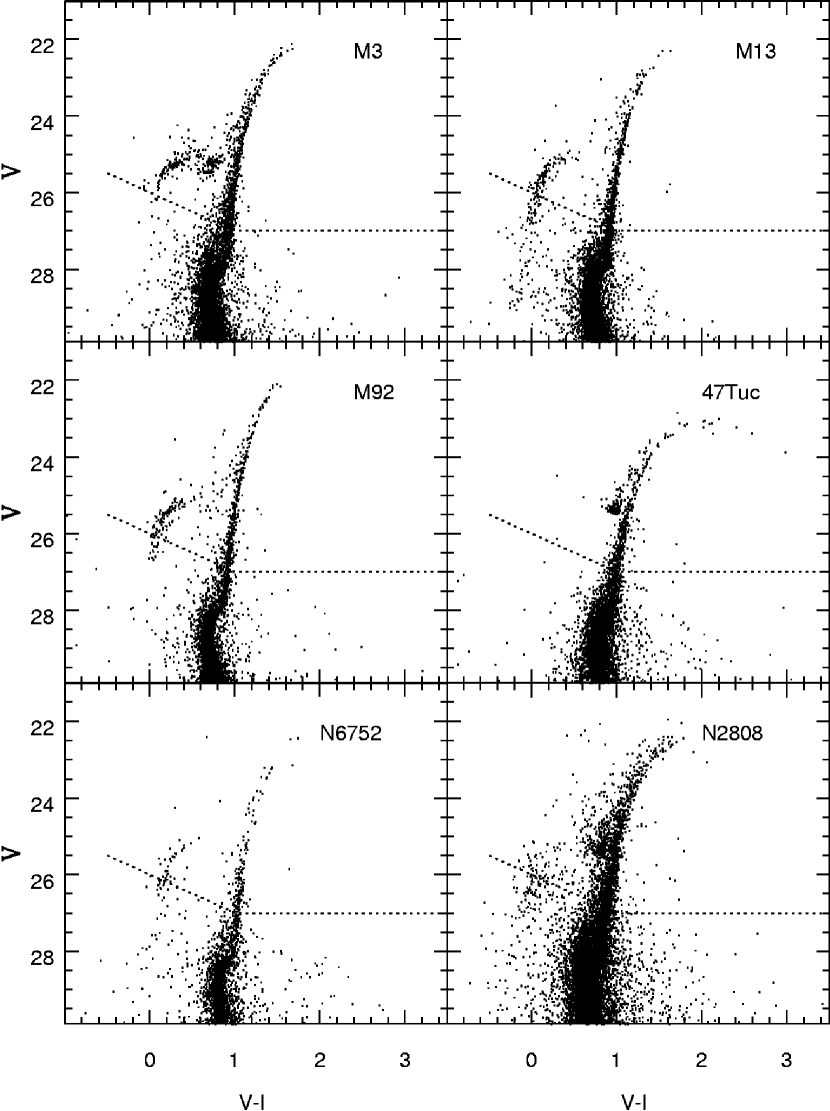
Figure 10: Example of how the CMDs of 6 among the best studied GGCs, namely M3, M13, M92, 47 Tuc, NGC6752 and NGC2808, would appear if placed at the distance of M31 and affected by the photometric cutoff that apply to our data set.

As we have seen e.g. in Fig. 2, the HB morphologies are generally similar to those of GGCs, the first parameter being metallicity. However, as clearly shown in Fig. 10, we note that the magnitude limits of our photometry would not allow us to detect extended blue tails that might reach as faint as $\sim$ 3 mag below the HB magnitude level. For example, a cluster such as NGC 6752, where the extended blue tail reaches as faint as the TO and contains a significant fraction of the total HB stellar population, would be measured as having a blue HB even though half such stars are undetected.

In order to test how the photometric cutoffs affect the appearence of the HBs, we have taken the well known and accurate CMDs of 6 of the best studied GGCs, namely M3, M13, M92, 47 Tuc, NGC6752 and NGC2808, and we have shifted the limiting magnitude cutoffs to the assumed distance to M31. The individual GGC reddening values have been taken from Harris (1996, update 2003). We have selected these clusters because they represent good cases of low, intermediate and high metallicity, of extended blue HB tail, and of a 2nd-parameter HB morphology. In Fig. 10 we show the results of this simulation. We note that a significant part of the HB population is lost when the HB is very blue and extends down to magnitudes as faint as the MS turnoff.

Therefore any conclusions based on the HB morphology must necessarily be qualitative. For example, we cannot hope to estimate the helium abundance $Y$ of our clusters using the $R$-method (Buzzoni et al.  1983), because this method relies on stellar counts in the RGB and HB evolutionary phases and completeness is an essential requirement.

However, more qualitative considerations are possible, for example we note that the HB morphologies of G119 and G105 are quite different even though they have very similar metallicity. This suggests the presence of 2nd-parameter clusters among our M31 clusters, as occurs in the MW GC system and in the Fornax dwarf spheroidal galaxy (Smith et al.  1996; Buonanno et al. 1998).

Quantitative considerations can also be possible, provided they are not affected by the magnitude cutoffs. For example, the magnitude level of the HB, V(HB), at the expected position of the instability strip (i.e. at approximately 0.3 $\lesssim(V-I)_{0}\lesssim$ 0.7), can be estimated with a good level of confidence and accuracy. These are the features that we analyse and discuss in the following sections.

3.3.1 The HB morphology: 2nd-parameter (2nd-P) effect

The morphology of the HB depends primarily on [Fe/H], metal-poor (-rich) clusters having predominantly blue (red) HBs. However in the Galaxy there are several cases where this general rule is not followed and the presence of a second (or more) parameter(s) must be invoked (see for references Fusi Pecci & Bellazzini 1997).

The 2nd-P candidate that has been most often suggested is age: for a given metallicity, age affects the HB morphology in the sense that older clusters have bluer HBs. However, at least in the case of NGC 2808, where the color distribution of the HB stars is bimodal and appears to be the sum of NGC362 and NGC288, the 2nd-P seems to be at work within the cluster itself. Therefore gross age differences alone are not responsible for this unusual HB (unless, of course, one assumes that the cluster contains at least two different generations of stellar populations, see for references D’Antona and Caloi 2004; also note the role of helium abundance as in $\omega$ Cen; Piotto et al.  2004).

A common approach to calculating a morphology derived HB index uses (B-R)/(B+V+R), where V indicates the number of variable HB stars (i.e. RR Lyraes) within the instability strip, and B and R the number of HB stars bluer and redder than the instability strip, respectively (Lee et al.  1994). Lacking a variable star census, we use the Mironov (1972) index, B/(B+R), where the boundary between the blue (B) and red (R) part of the HB is set at V-I = 0.50. When the stellar distribution along the HB is known with relatively poor accuracy and there is no knowledge of the variable stellar component, as is the case for our M31 GCs, the Mironov index is quite adequate to describe the HB morphology. We list in Table 8 the values of the Mironov index we have estimated for our M31 GCs.

We show in Fig. 11 the behavior of the Mironov index versus [Fe/H] (both taken from Table 8) for our GCs in M31 (shown as filled circles and identified with their names). For comparison, we show the GGCs for which the Mironov index is available (small open circles), and their general behavior as a shaded area whose mean line is drawn in analogy with the approach described by Lee et al.  (1994) for (B-R)/(B+V+R). As is well known, in the MW the 2nd-P phenomenon affects only clusters in the metallicity range approximately between [Fe/H]=–1.1 and –1.6.

The two cluster systems behave in a roughly similar way, except that the spread in HB type for the metal poor ($\rm[Fe/H]\sim-1.7$) clusters is striking, suggesting an offset from the Milky Way trend line. An underestimate of the B counts due to the loss of extended HB stars may explain part of this second parameter effect. However, G87, G287, and to some extent G11 and G219 appear to genuinely display the second parameter effect. As good candidates for the 2nd-P effect, we also note the pair G105 and G119, that have very similar metallicity: G105 falls nicely on the distribution defined by the GGCs, whereas G119 presents a distinctly redder HB morphology.

The Fornax dwarf galaxy shows the second parameter problem but at even lower metallicity than the M31 halo (Smith et al.  1996). The evidence for an age dispersion in the M31 halo field population (Brown et al.  2003) opens the question of whether the metal poor populations might have an age dispersion (note however that the strongest evidence for an intermediate age component is in the metal rich population). Buonnano et al.  (1998) report deep HST photometry reaching the turnoff point and place an age spread of $<$1 Gyr on the Fornax globular clusters; they further claim that the Fornax globular clusters have the same age as the oldest Milky Way clusters (e.g. M92). It would be valuable to undertake deeper observations of M31 globular clusters, at higher resolution, to explore the question of the second parameter problem and the relationship to the Milky Way clusters. Evidence for a systematic difference in the second parameter effect between the Milky Way, the Fornax dwarf, and M31 could point toward differences in age or chemistry. It has been argued that the Local Group experienced a common era of star formation as evidenced by the nearly identical age of the old halo globular clusters (see for example Harris et al.  1997; Rosenberg et al.  2002).

We may conclude that M31 exhibits the second parameter effect at lower metallicity than does the Milky Way, but not in extreme a sense as is evidenced in the Fornax dwarf.

3.3.2 The HB Luminosity-Metallicity Relation

The Population II distance scale is based on the absolute magnitude of local calibrators, i.e. the RR Lyrae stars, M_V(RR), which is known to be dependent on metallicity. This dependence has often been represented by a linear relation of the form $M_{V}=\alpha{\rm[Fe/H]}+\beta$, which seems to represent the observed behavior of these stars reasonably well (within the uncertainties), although some theoretical pulsation and evolution models suggest that a non-linear (quadratic?) relation might be more appropriate. Given the uncertainties of our estimates in the M31 GCs, the linear relation is quite adequate to our considerations. We refer the reader to Cacciari & Clementini (2003) for a recent and detailed review on this subject.

After a lengthly period of debate, $\alpha$ appears to be converging towards a value of $\sim$0.20-0.23: for example Gratton et al.  (2004) find 0.214$\pm$0.047 mag from the analysis of 98 RR Lyrae stars in the bar of the LMC, in general agreement with several recent independent estimates.

Also disagreement on the zero-point of this relation are finding a solution: once the most extreme (and less reliable) determinations are taken into account with the proper weight, the most recent and accurate results seem to converge on two sets of values that differ only by $\lesssim$0.05 mag. The “faint” solution converges toward $M_{V}$(RR)=0.59 mag at [Fe/H]=–1.5, and is mainly supported by the result of the HST trigonometric parallax on RR Lyr (Benedict et al. 2002) which we consider doubtful because of its rms error of $\pm$0.1 mag. On the other hand, the “bright’ solution converges toward $M_{V}$(RR)=0.55 mag at [Fe/H]=–1.5, and is mainly supported by the results of various studies on the LMC distance scale which are discussed and summarised as (m–M)₀(LMC)=18.515$\pm$0.085 by Clementini et al.  (2003).

Theoretical evolution and pulsation models agree with either estimate, within the respective errors.

We can hardly say there is any discrepancy left at all, therefore we assume that a relation,

$M_{V}=0.22{\rm[Fe/H]}+0.88$ (1)

with an rms error $\pm$0.05 mag, represents the behavior of the RR Lyrae stars quite reliably, and accurately enough for use in our M31 GCs. This relation corresponds to a distance to the LMC of (m–M)₀(LMC)=18.51 using Clementini et al.  (2003) data. We use it later to estimate $M_{V}$ and hence the distance (see case [C] in Table 8).

The CMDs of our M31 globular clusters, reaching about one magnitude below the HB, offer an interesting means to test the characteristics of the RR Lyrae stars in another galaxy (via the slope of the $M_{V}$(HB)-[Fe/H] relation) and derive the distance to M31, or, alternatively, to yield quantitative estimates on the spatial distribution of our clusters within the M31 spheroid.

The observed HB magnitude level V(HB)

We have estimated the apparent mean magnitude of the HB, V(HB), by a running box averaging method and adopted the V(HB) value at (V–I)₀=0.5, corresponding to the mid point of the instability strip that covers the range of (V–I)₀ colors approximately between 0.3 and 0.7.

For the metal-rich clusters ([Fe/H]$>$–1.0) where only the red HB clump is detected, we have used the $\langle V\rangle$ of the red HB clump corrected by +0.08 mag (see Paper I and references therein). We list the values of the observed V(HB) magnitudes in Table 8.

Typical photometric errors on the individual HB stars are about $\pm$0.05 mag (see Sect. 2.3), that become $\pm$0.02-0.01 mag when the average value V(HB) of 10-25 stars is taken. Considering an additional error of about $\pm$0.04 mag on the reddening values, the typical rms error we associate to V₀(HB) is $\pm$0.13 mag.

M_V(HB) and the distance to M31

We recall that in Sect. 3.2.2, as a result of the application of the RGB ridge line and global fitting methods (with fixed or free value for the reddening), we have derived for each cluster two estimates of distance (see Table 7 columns 5 and 8, reported also in Table 8 as cases [A] and [B], for the sake of convenience in the following discussion). These two sets are substantially compatible within the errors, with the exception of G33, G76, G302 and G322 where the two estimates differ by $\geq$0.15 mag, mostly because of significantly different values of reddening. Both methods yield an average distance modulus (m–M)₀(M31)=24.48$\pm$0.12 mag.

It is important to note that the values so obtained for M_V(HB) cannot be used to derive an independent M_V versus [Fe/H] relationship, as they actually reflect the relationship adopted by Harris (1996) to determine the distances of the GGCs used in the reference grid, namely $M_{V}=(0.15\pm 0.05){\rm[Fe/H]}+(0.76\pm 0.07)$. They can be used, however, to get some hint on the cluster locations and relative distances, in particular if the distance turns out systematically and significantly larger or smaller than the assumed value for M31.

However, there are other ways of deriving useful information on the M_V(HB) versus [Fe/H] relation, once the values for reddening, metallicity and HB apparent luminosity are known. In particular, we can derive an independent slope for the M_V versus [Fe/H] relationship, the zero-point depending on an assumed value of distance to M31.

By adopting the same distance to all the M31 clusters, i.e. (m–M)₀(M31)=24.47$\pm$0.03 (see Sect. 3.2.2) and the values of reddening, metallicity and V(HB) reported in Table 8 columns 3, 4 and 5, one can derive the corresponding values for M_V (reported under case [D] in Table 8) and the slope of the M_V versus [Fe/H] relationship independent of any other assumption. Since we assume that all clusters are at the same distance, the possible distance dispersion shows up as a larger dispersion in the M_V values.

In Fig. 12 we show the present sample of GCs (filled circles), along with the 8 GCs that were studied in Paper I and reanalysed here (open circles). The error-weighted least squares linear fit to these data, assuming errors on both [Fe/H] ($\pm$0.2 dex) and M_V(HB) ($\pm$0.13 mag), is shown in the figure and yields:

$M_{V}=(0.20\pm 0.09){\rm[Fe/H]}+(0.81\pm 0.13)$ (2)

As noted above, the large dispersion of the M_V values is due to the combination of two effects: i) the photometric errors and the uncertainties in the method applied to determine the average V(HB), and ii) the intrinsic luminosity dispersion due to the relative distances of the clusters within M31.

Concerning the slope of eq. (2), we note that the value 0.20 is in excellent agreement with the best estimates presently available (see eq.[1]), based on Galactic and LMC field RR Lyraes. We point out that the relatively low value of $\alpha\sim$ 0.13, that was derived in Paper I from the analysis of the first 8 M31 clusters, was obviously affected by large inaccuracies due to the very small sample size. That result is now revised with the addition of our new data and the re-evaluation of the clusters studied by Holland et al.  (1997), that have more than doubled the previous sample. As for the zero-point of eq. (2), it obviously depends on the assumption we have made on the distance to M31 that leads to M_V(HB)=0.51 at [Fe/H]=–1.5, corresponding to (m–M)₀(LMC)$\sim$18.55.

This finding leads us to conclude that the HB stars in M31 do indeed share the same physical behavior as in the MW and in the LMC, whether they belong to the field or to the GC stellar population. In particular, their luminosity varies as a function of metallicity in much the same way.

If we now assume that there is one “universal” M_V versus [Fe/H] relation, for example eq. (1) that we have derived before based on Galactic and LMC RR Lyraes, and calibrated on (m–M)₀(LMC)=18.51, we can derive the individual values of $M_{V}$(HB) irrespective of their distances. So doing, the dispersion due to the cluster location within the M31 spheroid now shows up through the derived distance moduli and not $M_{V}$(HB) (see case [C] in Table 8). The straight average value of the derived distance moduli in case (C) is 24.44$\pm$0.19 considering all 19 clusters, and 24.47$\pm$0.10 considering only the 14 clusters whose modulus deviates by less than 0.2 mag (i.e. 1$\sigma$) from the average. If we compare these distance moduli with those determined by Holland (1998) by fitting theoretical isochrones to the observed RGBs of 14 GCs, we note that the mean values are identical, i.e. 24.47. However, the individual values for the 11 clusters in common can differ randomly by up to 3$\sigma$ in a few cases. Considering that the two sets of results are based on different assumptions (e.g. on reddening and metallicity) and different methods (i.e. fitting the observed RGBs to theoretical isochrones instead of using template ridge lines), these differences are quite acceptable and point out the true uncertainties of these determinations.

From this exercise we conclude:

i) The mean distance to M31 agrees with the assumed value (m–M)₀(M31)=24.47 well within the error determinations, and consistently with (m–M)₀(LMC)=18.51-18.55.

ii) Several of our target clusters appear to lie off the assumed spheroidal distribution of radius $\sim$20 kpc (0.06 mag in distance modulus), i.e. at larger distances from the galactic center along the line of sight. Our measures indicate that G64, G76 and G322 are located on the near side of the spheroid, whereas G105, G351 and possibly G108 and G219 are located on the far side.

4 Summary and Conclusions

We have presented the results of our HST+WFPC2 observations in the filters F555W (V) and F814W (I) for 10 globular clusters in M31, and the reanalysis of 2 more clusters using HST archive data of comparable characteristics.

We obtain high quality CMDs down to approximately 1 magnitude below the HB. The principle sequences (HB and RGB) look similar to those seen in old Milky Way globular clusters.

We include also in our sample the CMDs for 8 clusters previously analyzed in Paper I, for a more general and comprehensive discussion of the M31 GC system characteristics; we conclude as follows:

1. We derive metallicities from the RGB ridgelines; these are in good agreement with those derived from integrated ground-based spectroscopic and/or photometric estimates.

2. The HB morphologies show the same behavior with [Fe/H] as in the Milky Way, including the possible presence of some 2nd-parameter clusters. An apparently peculiar HB morphology (bright red stars and a slanting HB) is shown to be due to blends of blue HB and RGB stars. We also correct for field contamination, when this is an issue. We observe the 2nd parameter effect at [Fe/H]=–1.6, more metal poor than is seen in the Galaxy, causing the trend of HB-type with [Fe/H] to be offset. A possible explanation for some of the metal-poor red-HB clusters that deviate most from the analogous distribution of GGCs is that they are a few Gyr younger, as estimated for G312 (Brown et al.  2004b).

3. The mean magnitude of the HB at the approximate location of the instability strip has been estimated, and a M_V(HB) versus [Fe/H] relationship has been derived. The range of metallicities spanned by the clusters make it possible to derive the slope of the M_V(HB) versus [Fe/H] relationship. We find this slope to be $\alpha=0.20\pm 0.09$, in excellent agreement with independent estimates based on Galactic and LMC RR Lyrae stars. This distance scale, based on (m–M)₀(M31)=24.47, is consistent with (m–M)₀(LMC)=18.55.

4. Relative distances could be estimated, and there is evidence that a few clusters lie on the foreground or background of the M31 main body.

Our results add further support to previous conclusions that the GC systems in the Galaxy and in M31 are basically very similar. However, a sample of 19 clusters represents less than 5% of the total cluster population in M31, and no firm conclusions can be drawn from such a sample, especially concerning relatively rare objects such as the 2nd-P clusters, or the possible presence of a younger population. Subtle differences between the Milky Way and M31 might follow from differing formation times or chemical evolution, but with such a small sample of M31 clusters, it is likely we are missing many interesting and crucial examples. A larger sample would place our observational description of the M31 cluster system at the same level as that of the Milky Way globular clusters just prior to the advent of CCD photometry. A larger sample would also give insight into the differences between the Milky Way and M31 that follow from possibly different ages and chemical evolution, essential qualities for a better understanding of the formation and evolution of galaxies like our own.

Table 1: The sample of M31 globular clusters observed with the HST and analysed in the present study. The data for the first 10 clusters are from the program GO-6671 (P.I Rich), the data for the last two clusters (G302 and G312) are from the program GO-5906 (P.I. Holland) and were taken from the HST archive.

Cluster		V	$(B-V)$	R	R	Obs. Date
Bo	G			(arcmin)	(kpc)
293	11	16.30	0.74	75.75	16.95	09/25/1999
311	33	15.44	0.97	57.59	12.88	02/26/1999
12	64	15.08	0.77	25.35	5.67	08/17/1999
338	76	14.25	0.81	45.03	10.07	01/11/1999
27	87	15.60	0.92	26.43	5.91	08/16/1999
30	91	17.39	1.93	24.86	5.56	08/16/1999
58	119	14.97	0.84	30.59	6.84	06/13/1999
233	287	15.76	0.85	35.45	7.93	09/26/1999
384	319	15.75	0.99	72.07	16.12	02/28/1999
386	322	15.55	0.90	61.80	13.83	01/10/1999
240	302	15.21	0.72	31.77	7.11	11/05/1995
379	312	16.18	0.85	49.75	11.13	10/31/1995

Notes:
1) The integrated photometric parameters V and (B–V) are from Galleti et al. (2004).
2) The values of $R$ are the projected galactocentric distances in arcmin (Col. 5) and kpc (Col. 6), on the assumption that (m-M)₀=24.47$\pm$0.03 mag (see Sect. 3.2.2).

Table 2: Information on the sampled population for each cluster. $Annulus$ represents the total area where photometry was performed. N_before and N_after are the number of stars before and after field subtraction. $R>$ represents the radius at which photometric blends become insignificant. N_noblend is the number of stars left after eliminating the photometric blends.

Cluster	$Annulus$	$L_{sam}/L_{tot}$	Nbefore	Nafter	$R>$	Nnoblend
	(arcsec)				(arcsec)
G11	1.00 $-$10.35	0.56	805	722	2.76	411
G33	1.70 $-$ 5.98	0.31	697	468	3.22	256
G64	1.84 $-$ 7.82	0.27	687	558	3.22	287
G76	2.76 $-$ 7.28	0.17	960	776	3.68	463
G87	1.56 $-$ 5.52	0.32	1123	836	2.30	610
G91	1.50 $-$ 3.50	0.21	193	133
G119	2.48 $-$ 5.52	0.12	745	484	3.22	386
G287	1.56 $-$ 4.74	0.29	756	587	2.76	219
G319	1.61 $-$10.12	0.27	420	397	1.84	365
G322	1.99 $-$ 5.98	0.21	534	345	2.30	302
G302	3.30 $-$12.00	0.21	712	409	6.00	229
G312	2.50 $-$12.00	0.20	375	288	3.00	263

Table 3: Reddening: collection of values from the literature, and adopted value.

Bo	G	Vet62	VdB69	FPC	BH	SFD	C85a	C85b	B00a	B00b	adopted	$\sigma$
(1)	(2)	(3)	(4)	(5)	(6)	(7)	(8)	(9)	(10)	(11)	(12)	(13)
293	11				0.08	0.06			0.12	0.12	0.09	0.03
311	33	0.02	0.46	0.22	0.06	0.06	0.29	0.21	0.32	0.26	0.18	0.11
12	64	-0.09	0.21	0.17	0.04	0.06	0.05	0.07	0.14	0.10	0.09	0.05
338	76	0.02	0.25		0.07	0.06			0.10	0.13	0.08	0.03
27	87	0.02	0.18	0.10	0.07	0.06	0.28	0.14	0.30	0.18	0.14	0.08
30	91	0.02	0.18	0.10	0.07	0.06	0.28	0.14	0.30	0.18	0.14	0.08
58	119	0.05	0.24	0.10	0.08	0.06			0.15	0.11	0.09	0.04
233	287	0.09			0.07	0.06	0.08	0.07	0.18	0.14	0.09	0.05
240	302	-0.01	0.21	0.10	0.09	0.06	0.06	0.13	0.08	0.06	0.08	0.02
379	312				0.09	0.06			0.04	0.09	0.07	0.02
384	319	-0.01			0.06	0.06			0.17	0.14	0.09	0.06
386	322				0.18	0.06	0.27	0.10	0.17	0.02	0.13	0.06
	1	0.16	0.19	0.10	0.05	0.06			0.01	0.08	0.07	0.02
6	58	0.07	0.08	0.10	0.04	0.06	0.18	0.11	0.16	0.13	0.10	0.05
343	105	-0.09			0.05	0.06			0.09	0.05	0.06	0.01
45	108	0.23	0.31	0.10	0.03	0.06	0.12	0.16	0.17	0.17	0.10	0.06
358	219	-0.16	0.15	0.10	0.04	0.06			-0.14	-0.04	0.06	0.08
225	280	0.08	0.09	0.10	0.07	0.06			0.20	0.14	0.10	0.05
405	351	-0.08	0.12		0.07	0.06			0.11	0.11	0.08	0.03
468					0.04	0.06			-0.12	-0.29	0.06	0.15

Columns:
(1): cluster identification from Battistini et al. (1987)
(2): cluster identification from Sargent et al. (1977)
(3): from Vetesnik (1962)
(4): from van den Bergh (1969)
(5): from Frogel et al. (1980)
(6): from the HI maps (Burstein & Heiles 1982)
(7): from the Galactic dust maps (Schlegel et al. 1998)
(8): from E(B-V)=-0.066S+1.17(B-V)-0.32 (Crampton et al. 1985), (B-V) from Galleti et al. (2004)
(9): from E(B-V)=-0.066S+1.17(B-V)-0.32 (Crampton et al. 1985), (B-V) from Crampton et al. (1985)
(10): from (B-V)₀=0.159[Fe/H]+0.92 (Barmby et al. 2000), [Fe/H] from Barmby et al. (2000), (B-V) from Galleti et al. (2004)
(11): from (B-V)₀=0.159[Fe/H]+0.92 (Barmby et al. 2000), [Fe/H] and (B-V) from Barmby et al. (2000)
(12): E(B-V) final adopted value
(13): dispersion of the mean

Table 4: Observed RGB ridge lines (I, V–I) for the M31 GCs considered in this analysis. For each cluster the ridge line is given from its RGB tip in steps of 0.1 mag. G91 is missing because no reliable ridge line could be defined (see Sect. 3.2.1).

		G11	G33	G64	G76	G87	G302	G312
I		$(V-I)$	$(V-I)$	$(V-I)$	$(V-I)$	$(V-I)$	$(V-I)$	$(V-I)$
20.45					1.994	1.925
20.55					1.928	1.879
20.65		1.652			1.866	1.835
20.75		1.616		1.494	1.808	1.794
20.85		1.582		1.466	1.752	1.754
20.95		1.546	1.721	1.440	1.700	1.717	1.591
21.05		1.513	1.694	1.415	1.650	1.681	1.563
21.15		1.482	1.665	1.392	1.603	1.647	1.535
21.25		1.454	1.639	1.369	1.560	1.615	1.507
21.35		1.428	1.612	1.348	1.518	1.585	1.479
21.45		1.404	1.589	1.328	1.479	1.557	1.453
21.55		1.383	1.567	1.309	1.443	1.529	1.427	1.920
21.65		1.362	1.548	1.292	1.410	1.504	1.404	1.842
21.75		1.343	1.529	1.275	1.378	1.479	1.384	1.772
21.85		1.325	1.511	1.260	1.348	1.456	1.367	1.716
21.95		1.307	1.494	1.245	1.321	1.435	1.350	1.673
22.05		1.290	1.480	1.232	1.296	1.415	1.334	1.638
22.15		1.274	1.465	1.220	1.273	1.397	1.319	1.608
22.25		1.258	1.452	1.209	1.251	1.379	1.305	1.577
22.35		1.242	1.439	1.197	1.230	1.362	1.292	1.548
22.45		1.228	1.427	1.186	1.211	1.347	1.279	1.522
22.55		1.214	1.415	1.175	1.194	1.332	1.267	1.498
22.65		1.202	1.404	1.164	1.178	1.318	1.256	1.477
22.75		1.190	1.392	1.153	1.163	1.305	1.244	1.455
22.85		1.179	1.381	1.143	1.149	1.293	1.234	1.432
22.95		1.168	1.370	1.134	1.137	1.282	1.224	1.410
23.05		1.158	1.358	1.124	1.126	1.271	1.214	1.389
23.15		1.149	1.347	1.115	1.114	1.262	1.205	1.370
23.25		1.139	1.336	1.107	1.104	1.252	1.196	1.352
23.35		1.131	1.325	1.098	1.094	1.243	1.187	1.336
23.45		1.122	1.315	1.090	1.085	1.235	1.178	1.319
23.55		1.114	1.306	1.082	1.076	1.226	1.170	1.302
23.65		1.106	1.296	1.074	1.067	1.218	1.161	1.284
23.75		1.098	1.287	1.067	1.058	1.211	1.153	1.267
23.85		1.090	1.279	1.060	1.050	1.203	1.144	1.250
23.95		1.083	1.272	1.052	1.041	1.195	1.136	1.235
24.05		1.077	1.264	1.046	1.034	1.188	1.127	1.221
24.15		1.071	1.257	1.039	1.026	1.181	1.119	1.208
24.25		1.065	1.250	1.033	1.017	1.173	1.110	1.197
24.35		1.059	1.243	1.027	1.006	1.165	1.102	1.187
24.45		1.053	1.236	1.021			1.094	1.178
24.55		1.046	1.230	1.015				1.169
24.65		1.039	1.223	1.010				1.162
24.75		1.032	1.216	1.004				1.154
24.85			1.210	0.999				1.147
24.95			1.203	0.994
25.05				0.989
25.15				0.985
25.25				0.981

Table 4: - continued -

		G119	G287	G319	G322
I		$(V-I)$	$(V-I)$	$(V-I)$	$(V-I)$
20.80				2.305	1.725
20.90				2.196	1.680
21.00			1.538	2.086	1.639
21.10		1.564	1.493	1.982	1.606
21.20		1.538	1.457	1.893	1.573
21.30		1.513	1.429	1.827	1.539
21.40		1.490	1.399	1.775	1.509
21.50		1.467	1.372	1.725	1.478
21.60		1.444	1.347	1.676	1.449
21.70		1.422	1.322	1.629	1.422
21.80		1.400	1.300	1.586	1.396
21.90		1.379	1.281	1.545	1.372
22.00		1.360	1.263	1.511	1.348
22.10		1.343	1.243	1.475	1.326
22.20		1.327	1.223	1.441	1.304
22.30		1.312	1.207	1.409	1.282
22.40		1.298	1.192	1.379	1.261
22.50		1.286	1.179	1.350	1.240
22.60		1.273	1.166	1.322	1.220
22.70		1.261	1.154	1.294	1.200
22.80		1.249	1.142	1.269	1.181
22.90		1.238	1.130	1.245	1.162
23.00		1.227	1.119	1.222	1.144
23.10		1.216	1.106	1.200	1.127
23.20		1.206	1.095	1.179	1.110
23.30		1.196	1.084	1.160	1.094
23.40		1.186	1.074	1.142	1.080
23.50		1.176	1.065	1.124	1.065
23.60		1.166	1.057	1.109	1.052
23.70		1.156	1.050	1.096	1.038
23.80		1.145	1.043	1.084	1.026
23.90		1.135	1.036	1.073	1.015
24.00		1.124	1.029	1.063	1.006
24.10		1.114	1.022	1.052	0.998
24.20		1.104	1.014	1.042	0.990
24.30		1.094	1.007	1.033	0.982
24.40		1.085	1.000	1.025	0.974
24.50		1.076	0.992	1.017	0.967
24.60		1.068	0.985	1.009	0.959
24.70		1.060	0.979	1.002	0.951
24.80		1.052	0.972	0.995	0.944
24.90		1.045	0.967	0.989	0.938
25.00		1.037	0.962	0.982	0.932
25.10		1.030	0.957	0.976	0.926
25.20		1.022		0.969	0.922
25.30		1.015		0.962	0.918
25.40				0.956
25.50
25.60
25.70
25.80

Table 5: Estimates of metallicity [Fe/H] for the M31 GCs considered in this analysis (upper group of 12 clusters) and those studied in Paper I (lower group of 8 clusters). The metallicity in the ZW84 and CG97 metallicity scales were calculated according to Saviane et al.  (2000, Table 6). For G280 and G351 metallicities could only be derived in the CG97 scale (see Ferraro et al.  1999, Table 4).

Bo	G	S	RGBZW	RGBCG	Ridge	Ridge	HBK	P	B	Adopted	$\sigma$
		(1)	(2)	(3)	(4)	(5)	(6)	(7)	(8)	(9)	(10)
293	11	8.23	-1.70	-1.33	-1.6	-1.7	-1.89		-2.13	-1.80	0.21
311	33	8.47	-1.75	-1.39	-1.6	-1.75	-1.74	-1.96	-1.88	-1.78	0.13
12	64	8.45	-1.75	-1.39	-1.8	-1.9	-1.81	-1.65	-2.17	-1.85	0.18
338	76	4.67	-0.84	-0.77	-1.3	-1.3	-1.34	-1.46	-1.41	-1.28	0.22
27	87	8.37	-1.79	-1.37	-1.4	-1.66	-1.64		-1.72	-1.64	0.15
30	91							-0.39
58	119	7.06	-1.41	-1.06	-1.3	-1.4	-1.45		-1.35	-1.38	0.06
233	287	7.81	-1.60	-1.22	-1.6	-1.6	-1.59			-1.60	0.01
240	302	7.91	-1.62	-1.25	-1.4	-1.66	-1.76		-1.97	-1.68	0.21
379	312	3.25	-0.50	-0.76	-0.51	-0.6	-0.70		-0.88	-0.64	0.16
384	319	3.87	-0.65	-0.75	-0.7	-0.7	-0.66		-1.62	-0.87	0.42
386	322	4.62	-0.83	-0.77	np	-1.2	-1.21	-1.62	-0.57	-1.09	0.40
	1	4.21	-0.73	-0.75	-1.0	-0.9	-1.08		-1.23	-0.99	0.19
6	58	3.25	-0.50	-0.76	-0.6	-0.6	-0.57	-0.58	-0.59	-0.57	0.04
343	105	7.34	-1.48	-1.12	-1.45	-1.5	-1.49		-1.29	-1.44	0.09
45	108	4.78	-0.87	-0.78	-0.6	-0.9	-0.94	-1.05	-0.76	-0.85	0.16
358	219	8.85	-1.84	-1.50	-1.91	-1.91	-1.83		-2.09	-1.92	0.10
225	280	3.82		-0.40	-0.35	-0.71	-0.70	-0.67	-0.37	-0.56	0.18
405	351	5.54		-0.88	-1.65	-1.70	-1.80		-1.93	-1.77	0.12
468		4.23	-0.74	-0.75	-0.7	-0.75				-0.73	0.03

Notes:
(1): The $S$ parameter is defined in the (V,V–I) plane, except for clusters G280 and G351 where the $S_{2.0}$ parameter, defined in the (V,B–V) plane, is reported instead (Saviane et al.  2000);
(2): from the $S$-parameter, ZW84 metallicity scale;
(3): from the $S$-parameter, CG97 metallicity scale;
(4): from the comparison of the RGB ridge lines with GGC templates, using the adopted E(B-V);
(5): from the comparison of the RGB ridge lines with GGC templates, using E(B-V) as a free parameter;
(6): spectroscopic (Huchra et al. 1991; Barmby et al. 2000)
(7): spectroscopic (Perrett et al. 2002)
(8): photometric (V–K integrated colors, Bonoli et al. 1987)
(9): Adopted values (see Sect. 3.2.3)
(10): Dispersion of the mean (see Sect. 3.2.3)

Table 6: Reference grid of template Galactic GCs. Metallicities are from Zinn (1985); all other parameters are from Harris (1996, update 2003).

Cluster	${\rm[Fe/H]}_{ZW84}$	$E(B-V)$	$(m-M)_{V}$
M15	-2.15	0.10	15.37
NGC6397	-1.91	0.18	12.36
NGC5824	-1.87	0.13	17.93
M13	-1.65	0.02	14.48
M3	-1.66	0.01	15.12
M5	-1.40	0.03	14.46
47 Tuc	-0.71	0.04	13.37
NGC6356	-0.62	0.28	16.77
NGC6624	-0.35	0.28	15.36
NGC6553	-0.29	0.63	15.83

Table 7: Metallicities and individual distance moduli using adopted and fitted reddening. The adopted values are described in Sect. 3.1 and are listed in Table 3. The fitted values are described in Sect. 3.2.2.

Bo	G	E(B-V)ad	[Fe/H]	(m-M)0	E(B-V)free	[Fe/H]	(m-M)0
293	11	0.09	-1.6	24.52	0.11	-1.7	24.48
311	33	0.18	-1.6	24.53	0.25	-1.75	24.30
12	64	0.09	-1.8	24.40	0.11	-1.9	24.30
338	76	0.08	-1.3	24.20	0.05	-1.3	24.35
27	87	0.14	-1.4	24.55	0.18	-1.66	24.55
58	119	0.09	-1.3	24.35	0.12	-1.4	24.35
233	287	0.09	-1.6	24.36	0.08	-1.6	24.42
240	302	0.08	-1.4	24.60	0.14	-1.66	24.40
379	312	0.07	-0.51	24.53	0.11	-0.6	24.44
384	319	0.09	-0.7	24.43	0.04	-0.7	24.55
386	322	0.13	np	24.30	0.04	-1.2	24.50
	1	0.07	-1.0	24.46	0.04	-0.9	24.55
6	58	0.10	-0.6	24.57	0.09	-0.6	24.56
343	105	0.06	-1.45	24.68	0.07	-1.5	24.68
45	108	0.10	-0.6	24.55	0.15	-0.9	24.55
358	219	0.06	-1.91	24.52	0.05	-1.91	24.58
225	280	0.10	-0.35	24.53	0.15	-0.71	24.40
405	351	0.08	-1.65	24.73	0.09	-1.70	24.68
468		0.06	-0.7	24.48	0.08	-0.75	24.50

Table 8: Adopted reddenings, metallicities and distances from the RGB morphology (see Sect. 3.1.2). The Mironov index B/(B+R) is discussed in Sect. 3.2.1; the V(HB) magnitudes and the distance moduli are discussed in Sect. 3.2.2.

Cluster		$E(B-V)$	[Fe/H]	V(HB)	MV	$(m-M)_{0}$	MV	$(m-M)_{0}$	MV	$(m-M)_{0}$	MV	$(m-M)_{0}$	B/(B+R)
Bo	G				(A)		(B)		(C)		(D)
293	11	0.09	-1.80	25.23	0.43	24.52	0.41	24.48	0.48	24.47	0.48	24.47	0.84
311	33	0.18	-1.78	25.49	0.40	24.53	0.41	24.30	0.49	24.45	0.46	24.47	0.44
12	64	0.09	-1.85	24.92	0.24	24.40	0.28	24.30	0.47	24.17	0.17	24.47	0.69
338	76	0.08	-1.28	24.94	0.49	24.20	0.43	24.35	0.60	24.09	0.22	24.47	0.43
27	87	0.14	-1.64	25.51	0.53	24.55	0.40	24.55	0.52	24.56	0.61	24.47	0.17
58	119	0.09	-1.38	25.21	0.58	24.35	0.49	24.35	0.58	24.35	0.46	24.47	0.27
233	287	0.09	-1.60	25.24	0.60	24.36	0.57	24.42	0.53	24.43	0.49	24.47	0.35
240	302	0.08	-1.68	25.14	0.29	24.60	0.31	24.40	0.51	24.38	0.42	24.47	0.53
379	312	0.07	-0.64	25.50	0.75	24.53	0.72	24.44	0.74	24.55	0.81	24.47	0.00
384	319	0.09	-0.87	25.46	0.75	24.43	0.79	24.55	0.69	24.49	0.71	24.47	0.00
386	322	0.13	-1.09	25.10	0.40	24.30	0.48	24.50	0.64	24.06	0.23	24.47	0.41
	1	0.07	-0.99	25.15	0.47	24.46	0.48	24.55	0.66	24.27	0.46	24.47	0.19
6	58	0.10	-0.57	25.46	0.58	24.57	0.62	24.56	0.75	24.40	0.68	24.47	0.03
343	105	0.06	-1.44	25.47	0.60	24.68	0.57	24.68	0.56	24.73	0.81	24.47	0.74
45	108	0.10	-0.85	25.62	0.76	24.55	0.61	24.55	0.69	24.62	0.84	24.47	0.14
358	219	0.06	-1.92	25.27	0.56	24.52	0.54	24.58	0.46	24.63	0.61	24.47	0.78
225	280	0.10	-0.56	25.52	0.68	24.53	0.66	24.40	0.76	24.45	0.74	24.47	0.15
405	351	0.08	-1.77	25.43	0.45	24.73	0.47	24.68	0.49	24.69	0.71	24.47	0.71
468		0.06	-0.73	25.41	0.74	24.48	0.66	24.50	0.72	24.51	0.75	24.47	0.00

Notes:
(A): adopted reddening (column 2 this table), best fit distance, derived $M_{V}$;
(B): best fit reddening and distance, derived $M_{V}$;
(C): $M_{V}$ from eq. (1), adopted reddening (column 2 this table), derived distance;
(D): adopted distance (24.47) and reddening (column 2 this table), derived $M_{V}$ and hence eq. (2).

Figure 1: I band (F814W) images of the 12 M31 GCs analysed in the present study. All of the $20^{\prime\prime}\times 20^{\prime\prime}(=80pc)$ subrasters are from PC frames except for those of G91, G302 and G312 which fell on the WFC. The clusters are displayed in the order of Fig. 2. Available in $jpeg$ format.

Figure 5: CMD of G64: the top left panel shows the entire photometric data set, the other panels show the stars measured in progressively external areas of radius $r$ (in pixels). The brightest and reddest part of what might look like the HB in the total CMD progressively disappears in the CMDs of more external less crowded areas, thus indicating that these are not true stars but photometric blends. The radius at which the blending becomes irrelevant is at $r\sim$70 px.

Figure 6: Completeness curves for G64 over different radial annuli. Dotted: 45 $<r<$ 60 px; dashed: 60 $<r<$ 80 px; full: $r>$ 80 px. See sect. 2.5 for discussion.

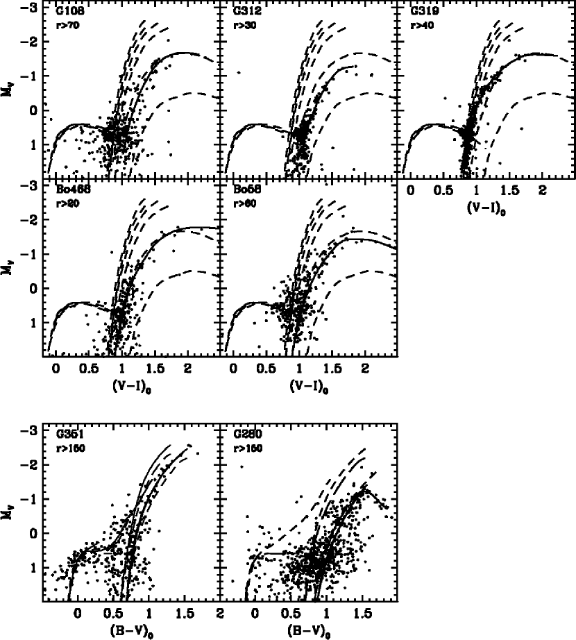
Figure 9: RGB ridge lines of our GCs (shown as solid lines), plotted individually along with the grid of GGC RGB templates (shown as dashed lines). The (M_V/(V-I)₀ templates are for: NGC6553, 47 Tuc, M5, M3, NGC6397 and M15; the (M_V/(B-V)₀ templates are for: M15, NGC5824, M13, M5, 47 Tuc, NGC6356, and NGC6624 (see Table 6).

Figure 11: HB morphology, as described by the Mironov index B/(B+R), as a function of [Fe/H]. The corresponding behavior of the GCs in the MW (open circles) and in Fornax (open squares) is also shown for comparison (see Sect. 3.3.1). The 2nd parameter effect in M31 would appear to occur at lower metallicity than is the case for the Galaxy, consistent with expectations if the cluster system is younger.

Figure 12: Mean M_V(HB) as a function of [Fe/H] for the present 11 GCs (filled circles) and the 8 GCs that were studied in Paper I (open circles). The line represents the best linear fit M_V(HB)=(0.20$\pm$0.09)[Fe/H]+(0.81$\pm$0.13), rms error of the fit $\sigma$=0.18. Some of the most discrepant clusters may be physically located at a distance different from that of the main M31 cluster population (see Sect. 3.3.2).

References

- Ajhar et al. (1996) Ajhar, E. A., Grillmair, C. J., Lauer, T. R., Baum, W. A., et al.: 1996, AJ, 111, 1110
- Ashman et al. (1998) Ashman, K.M. & Zepf, S.E. 1998, in Globular Cluster Systems, (Cambridge: Cambridge University Press)
- Barmby & Huchra (2001) Barmby, P. & Huchra, J.P. 2001, AJ, 122, 2458
- Barmby et al. (2000) Barmby, P., Huchra, J.P., Brodie, J.P., et al. 2000, AJ, 119, 727
- Barmby et al. (2001) Barmby, P., Huchra, J.P. & Brodie, J.P. 2001, AJ, 121, 1482
- Barmby et al. (2002) Barmby, P., Holland, S. & Huchra, J.P. 2002, AJ, 123, 1937
- Barmby (2003) Barmby, P., 2003, in Extragalactic Globular Cluster Systems, ESO Workshop, ed. M. Kissler-Patig, Springer-Verlag, p.143
- Battistini et al. (1987) Battistini, P., Bònoli, F., Braccesi, A., Federici, L., Fusi Pecci, F., Marano, B. & Borngen, F. 1987, A&AS, 67, 447
- Bekki et al. (2002) Bekki, K., Couch, W.J., Drinkwater, M.J. & Gregg, M.D. 2002, ApJ, 557, L39
- Bellazzini et al. (1995) Bellazzini, M., Pasquali, A., Federici, L., Ferraro, F.R. & Fusi Pecci, F. 1995, ApJ, 439, 687
- Bellazzini et al. (1999) Bellazzini, M., Ferraro, F.R. & Buonanno, R. 1999a, MNRAS, 304, 633
- Bellazzini et al. (1999) Bellazzini, M., Ferraro, F.R. & Buonanno, R. 1999b, MNRAS, 307, 619
- Bellazzini et al. (2001) Bellazzini, M., Ferraro, F.R. & Pancino, E. 2001, ApJ, 556, 635
- Bellazzini et al. (2003) Bellazzini, M., Cacciari, C., Federici, L., Fusi Pecci, F. & Rich, M. 2003, A&A, 405, 867
- Benedict et al. (2002) Benedict, G.F. et al. 2002, AJ, 123, 473
- Bonoli et al. (1987) Bonoli, F., Delpino, F.E., Federici, L. & Fusi Pecci, F., 1987, A&A185, 25
- Brown et al. (2003) Brown, T.M., Ferguson, H.C., Smith, E., Kimble, R.A., Sweigart, A.V., Renzini, A., Rich, R.M. & VandenBerg, D.A. 2003, ApJ, 592, L17
- Brown et al. (2004a) Brown, T.M., Ferguson, H.C., Smith, E., Kimble, R.A., Sweigart, A.V., Renzini, A., Rich, R.M. & VandenBerg, D.A. 2004a, AJ, 127, 2738
- Brown et al. (2004b) Brown, T.M., Ferguson, H.C., Smith, E., Kimble, R.A., Sweigart, A.V., Renzini, A., Rich, R.M. & VandenBerg, D.A. 2004b, ApJ, 613, L125
- Buonanno et al. (1983) Buonanno, R., Buscema, G., Corsi, C.E. & Iannicola G. 1983, A&A126, 278
- Buonanno et al. (1998) Buonanno, R., Corsi, C.E., Zinn, R., Fusi Pecci, F., Hardy, E. & Suntzeff, N.B. 1998, ApJ, 501, L33
- Burstein & Heiles (1982) Burstein, D. & Heiles, C. 1982, AJ, 87, 1165
- Burstein et al. (1984) Burstein, D., Faber, S.M., Gaskell, C.M. & Krumm, N. 1984, ApJ, 287, 586
- Burstein et al. (2004) Burstein, D., Li, Y., Freeman, K.C., Norris, J.E. et al. 2004, ApJ, 614, 158
- Buzzoni et al. (1983) Buzzoni, A. et al. 1983, A&A, 128, 94
- Cacciari & Clementini (2003) Cacciari, C. & Clementini, G. 2003, in Stellar Candles for the Extragalactic Distance Scale, Lect. Notes in Phys. Vol. 635, eds. D. Alloin and W. Gieren, Springer-Verlag, p. 105
- Carretta & Gratton (1997) Carretta & Gratton 1997, A&AS, 121, 95 (CG97)
- Choi et al. (2002) Choi, P.I., Guhathakurta, P. & Johnston, K.V. 2002, AJ, 124, 310
- Clementini et al. (2001) Clementini, G., Federici, L., Corsi, C.E., Cacciari, C., Bellazzini, M. & Smith, H.A. 2001, ApJ, 559, L109
- Clementini et al. (2003) Clementini, G., Gratton, R.G., Bragaglia, A., Carretta, E., Di Fabrizio, L. & Maio, M. 2003, AJ, 125, 1309
- Corsi et al. (2000) Corsi, C.E., Rich, M.R., Cacciari, C., Federici, L. & Fusi Pecci, F. 2000, in A Decade of HST Science, Ed.s M. Livio, K. Noll & M. Stiavelli, STScI Symp. Series Vol. 14, p. 28
- Crampton et al. (1985) Crampton, D., Cowley, A.P., Shade, D., & Chayer, P. 1985, ApJ, 288, 494
- D’Antona & Caloi (2004) D’Antona, F. & Caloi, V. 2004, ApJ, 611, 871
- Di Stefano et al. (2002) Di Stefano, R., Kong, A.K.H., Garcia, M.R., Barmby, P., Greiner, J., Murray, S.S. & Primini, F.A. 2002, ApJ, 570, 618
- Dolphin (2000) Dolphin, A. E. 2000, PASP, 112, 1383
- Djorgovski et al. (1997) Djorgovski, S.G., Gal, R.R., McCarthy, J.K., Cohen, J.G., de Carvalho, R.R., Meylan, G., Bendinelli, O. & Parmeggiani, G. 1997, ApJ, 474, L19
- Djorgovski et al. (2003) Djorgovski,S.G., Côté, P., Meylan, G., Castro, S., Federici, L., et al. 2003 in New horizons in globular cluster astronomy, eds. G.Piotto, G. Meylan, S.G. Djorgovski and M. Riello, A.S.P. Conf. Ser. Vol. 296, p. 479
- Durrell et al. (2001) Durrell, P.R., Harris, W.E. & Pritchet, C.J. 2001, AJ, 121, 2557
- Ferguson et al. (2002) Ferguson, A.M.N., Irwin, M.J., Ibata, R.A., Lewis, G.F. & Tanvir, N.R. 2002, AJ, 124, 1452
- Ferraro et al. (1999) Ferraro, F.R., Messineo, M., Fusi Pecci, F., De Palo, M.A., Straniero, O., Chieffi, A. & Limongi, M., 1999, AJ, 118, 1738
- Freedman et al. (2001) Freedman, W.L. et al. 2001, ApJ, 553, 47
- Frogel et al. (1980) Frogel, J.A., Persson, S.E. & Cohen, J.G. 1980, ApJ, 240, 785
- Fusi Pecci et al. (1994) Fusi Pecci, F., Battistini, P., Bendinelli, O., Bonoli, F., Cacciari, C., Djorgovski, S.G., Federici, L., Ferraro, F.R., Parmeggiani, P., Weir, N., & Zavatti, F. 1994, A&A, 284, 349
- Fusi Pecci et al. (1996) Fusi Pecci, F., Buonanno, R., Cacciari, C., Corsi, C. E., Djorgovski, S. G., Federici, L., Ferraro, F. R., Parmeggiani, G., Rich, R. M. 1996, AJ, 112, 1461 (Paper I)
- Fusi Pecci & Bellazzini (1997) Fusi Pecci, F. & Bellazzini, M. 1997, in the Third Conf. on Faint Blue Stars ed. A.G.D. Philip, J. Liebert, & R.A. Saffer (Schenectady: L. Davis Press), 255
- Fusi Pecci et al. (2004) Fusi Pecci, F., Bellazzini, M., Buzzoni, A., De Simone, E., Federici, L. & Galleti, S. 2004, AJ, submitted
- Galleti et al. (2004) Galleti, S., Federici, L., Bellazzini, M., Fusi Pecci, F. & Macrina, S. 2004, A&A, 416,917
- Gratton et al. (2004) Gratton, R.G., Bragaglia, A., Clementini, G., Carretta, E., Di Fabrizio, L., Maio, M. & Taribello, E. 2004, A&A, 421, 937
- Guarnieri et al. (1998) Guarnieri, M.D., Ortolani, S., Montegriffo, P., Renzini, A., Barbuy, B., Bica, E. & Moneti, A. 1998, A&A, 331, 70
- Harris (1996) Harris, W.E. 1996, AJ, 112, 1487 (update 2003, http://physun.physics.mcmaster.ca/Globular.html)
- Harris et al. (1997) Harris, W.E., Bell, R.A., Vandenberg, D.A., Bolte, M., Stetson, P.B. et al. 1997, AJ, 114, 1030
- Hartwick (1968) Hartwick, F.D.A., 1968, ApJ, 154, 475
- Holland (1998) Holland, S. 1998, AJ, 115, 1916
- Holland et al. (1997) Holland, S., Fahlman, G.G., Richer, H.B. 1997, AJ, 114, 1488
- Huchra et al. (1991) Huchra, J.P., Brodie, J.P. & Kent, S.M. 1991, ApJ, 370, 495
- Ibata et al. (1994) Ibata, R.A., Gilmore, G., & Irwin, M.J. 1994, Nature, 370, 194
- Ibata et al. (2001) Ibata, R.A., Irwin, M.J., Lewis, G.F., Ferguson, A.M.N. & Tanvir, N.R. 2001, Nature, 412, 49
- Jablonka (1992) Jablonka, P. , Alloin, D. & Bica. E. 1992, A&A, 260, 97
- Jablonka et al. (2000) Jablonka, P., Courbin, F., Meylan, G., Sarajedini, A., Bridges, T.J. & Magain, P. 2000, A&A, 359, 131
- Joshi et al. (2003) Joshi, Y.C., Pandey, A.K., Narasimha, D., Sagar, R. & Giraud-H raud, Y. 2003, A&A, 402, 113
- Lee et al. (1994) Lee, Y.-W., Demarque, P. & Zinn, R. 1994, ApJ, 423, 248
- Lupton (1989) Lupton, R. H. 1989, AJ, 97, 1350
- McClure & Racine (1969) McClure, R.D. & Racine, R. 1969, AJ, 74, 1000
- McConnachie et al. (2004) McConnachie, A.W., Irwin, M.J., Ferguson, A.M.N., Ibata, R.A., Lewis, G.F. & Tanvir, N. 2004, MNRAS, in press (astro-ph0410489)
- McLaughlin (2000) McLaughlin, D.E. 2000, ApJ, 539, 618
- Meylan et al. (2001) Meylan, G., Sarajedini, A., Jablonka, P., Djorgovski, S.G., Bridges, T.J & Rich, R.M. 2001, AJ, 112, 830
- Mighell et al. (1996) Mighell, K.J., Rich, R.M., Shara, M. & Fall. S.M. 1996, AJ, 111, 2314
- Mironov (1972) Mironov, A.V. 1972, Soviet Astronomy, 16, 105
- Moffat (1969) Moffat, A.F.J. 1969, A&A, 3, 455
- Morrison et al. (2004) Morrison, H.L., Harding, P., Perrett, K. & Hurley-Keller, D. 2004, ApJ, 603, 87
- Peterson et al. (2003) Peterson, R.C., Carney, B.W., Dorman, B., Green, E.M., Landsman, W., Liebert, J., O’Connell, R.W. & Rood, R.T. 2003, ApJ, 588, 299
- Perrett et al. (2002) Perrett, K.M., Bridges, T.J., Hanes, D.A., Irwin, M.J., Brodie, J.P., Carter, D., Huchra, J.P. & Watson, F.G. 2002, AJ, 123, 2490
- Piotto et al. (2002) Piotto, G., King, I.R., Djorgovski, S.G., Sosin, C., Zoccali, M., et al. 2002, A&A, 391, 945
- Piotto et al. (2004) Piotto, G. et al. 2004, ApJ, in press (astro-ph/0412016)
- Rich (2004) Rich, R.M. 2004, in Origin and Evolution of the Elements, ed. A. McWilliam and M. Rauch, Carnegie Obs. Ap. Series Vol. 4, p. 258 (Cambridge: Cambridge Univ. Press)
- Rich et al. (1996) Rich, R.M., Mighell, K.J., Freedman, W., & Neill, J.D. 1996, AJ, 111, 768
- Rich et al. (2001) Rich, R.M., Corsi, C.E., Bellazzini, M., Federici, L., Cacciari, C. & Fusi Pecci, F. 2001, in Extragalactic Star Clusters, eds. E. Grebel, D. Geisler and D. Minniti, IAU. Symp. 207, p. 140
- Rosenberg et al. (1999) Rosenberg, A., Saviane, I., Piotto, G. & Aparicio, A. 1999, AJ, 118, 2306
- Rosenberg et al. (2000a) Rosenberg, A., Piotto, G., Saviane, I. & Aparicio, A. 2000a, A&AS, 144, 5
- Rosenberg et al. (2000b) Rosenberg, A., Aparicio, A., Saviane, I. & Piotto, G. 2000b, A&AS, 145, 451
- Rosenberg et al. (2002) Rosenberg, A., Aparicio, A., Piotto, G., & Saviane, I. 2002, Ap&SS 281, 125
- Saito & Iye (2000) Saito, Y. & Iye, M. 2000, ApJ, 535, L95
- Sarajedini (1994) Sarajedini, A., 1994, AJ, 107, 618
- Sargent et al. (1977) Sargent, W.L.W., Kowal, C.T., Hartwick, F.D.A. & van den Bergh, S. 1977, AJ, 82, 947
- Saviane et al. (2000) Saviane, I., Rosenberg, A., Piotto, G. & Aparicio, A. 2000, A&A, 355, 966
- Schlegel et al. (1998) Schlegel, D.J., Finkbeiner, D.P. & Davis, M. 1998, AJ, 500, 525
- Smith et al. (1996) Smith, E.O., Neill, J.D., Mighell, K.J., & Rich, R.M. 1996, AJ, 111, 1596
- Stanek & Garnavich (1998) Stanek, K.Z. & Garnavich, P.M. 1998, ApJ, 503, L131
- Staneva et al. (1996) Staneva, A., Spassova, N. & Golev, V. 1996, A&AS, 116, 447
- Stephens et al. (2001) Stephens, A.W., Frogel, J.A., Freedman, W., Gallart, C., Jablonka, P., Ortolani, S., Renzini, A., Rich, R.M., Davies, R. 2001, AJ, 121, 2597
- van den Bergh (1969) van den Bergh, S. 1969, ApJS 19,145
- van den Bergh (2000) van den Bergh, S. 2000, PASP, 112, 932
- van den Bergh (2003) van den Bergh, S. 2003, in The Local Group as an Astrophysical Laboratory, (Cambridge: Cambridge Univ. Press), in press (astro-ph/0305042)
- van Speybroeck et al. (1979) van Speybroeck, L. et al. 1979, ApJ, 234, L45
- Vetesnik (1962) Vetesnik, M. 1962, Bull.Astron.Inst.Czechoslovakia.,13,180
- Zinn & West (1984) Zinn, R.J. & West, M.J. 1984, ApJS, 55, 45 (ZW84)
- Zinn (1985) Zinn, R.J. 1985, ApJ, 293, 424
- Trudolyubov & Priedhorsky (2004) Trudolyubov, S. & Priedhorsky, W. 2004, ApJ, in press (astro-ph/0402619)