A fresh look at the unstable simulations of Bondi-Hoyle-Lyttleton accretion

The instability of Bondi-Hoyle-Lyttleton accretion, observed in numerical simulations, is analyzed through known physical mechanisms and possible numerical artefacts. The mechanisms of the longitudinal and transverse instabilities, established within the accretion line model, are clarified. They cannot account for the instability of BHL accretion at moderate Mach number when the pressure forces within the shock cone are taken into account. The advective-acoustic instability is considered in the context of BHL accretion when the shock is detached from the accretor. This mechanism naturally explains the stability of the flow when the shock is weak, and the instability when the accretor is small. In particular, it is a robust proof of the instability of 3D accretion when $\gamma=5/3$ if the accretor is small enough, even for moderate shock strength (${\cal M}\sim 3$). The numerical artefacts that may be present in existing numerical simulations are reviewed, with particular attention paid to the advection of entropy/vorticity perturbations and the artificial acoustic feedback from the accretor boundary condition. Several numerical tests are proposed to test these mechanisms.

1 Introduction

The phenomena described by numerical simulations are usually highly simplified compared to the physical reality. However simplified, these phenomena are sometimes complicated enough to challenge our ability to understand them. The flow of gas onto a gravitating accretor moving supersonically is a classic astrophysical problem (Hoyle & Lyttleton 1939, Bondi & Hoyle 1944) which is relevant in many astrophysical contexts such as wind fed X-ray binaries, supermassive black holes, star formation, and also galaxies in a cluster (see the recent review by Edgar 2004). Early numerical simulations in 2D (Matsuda et al. 1987, Fryxell & Taam 1988) revealed that this flow is unstable. 3D simulations (Matsuda et al. 1991, Ruffert & Arnett 1994) confirmed the unstable character of the flow, displaying however a weaker variability than in 2D. The instability is not understood even in the simple case of an ideal uniform gas. Is this instability physical, or numerical? Is it the same instability mechanism in 2D and 3D? How can this unstable behaviour be extrapolated to small accretor sizes, which are relevant for wind fed X-ray binaries but out of reach of numerical simulations? Some authors recently doubted that this instability is physical (Pogorelov, Ohsugi & Matsuda 2000). The most recent relativistic simulations by Font & Ibanez (1998a, 1998b) and Font, Ibanez & Papadopoulos (1999) also showed stable flows. What about the published instability mechanisms which have been proposed over the years? What is left of the longitudinal and transverse instabilities of the accretion line (Cowie 1977, Soker 1990, 1991), the ”relatively simple” mechanism based on the shock opening angle by Livio et al. (1991), the ”vortex shedding in the Von Karman manner” (Koide et al. 1991, Matsuda et al. 1991, 1992)? The present uncertain situation reveals how unconvincing the proposed mechanisms were. Some were inconclusive, lacked quantitative criteria, and others might also have been incompletely understood. The present work aims at clarifying the different instability mechanisms and confront them with existing numerical simulations, paying particular attention to possible numerical artefacts.
The general trends based on the existing simulations, and the proposed mechanisms are recalled in Sect. 2. The longitudinal and transverse instabilities of the accretion line are revisited in Sect. 3 and Sect. 4. The advective-acoustic instability is adapted to the BHL flow in Sect.  5. This enables a new look at the simulations in Sect. 6, in an attempt to reconcile them. The basis of new simulations, free of numerical artefacts, testing these ideas, is described in Sect. 7. For the sake of the clarity of the paper, the main text contains only the most important equations, which summarize the analytical arguments proven in appendices A to H.

2 An overview of existing simulations of BHL accretion and proposed instability mechanisms

2.1 Numerical simulations are numerous

Table 1: Overview of the published numerical simulations of BHL accretion using a polytropic equation of state and a totally absorbing accretor: plane accretion in 2D, 3D axisymmetric accretion and full 3D accretion. The first column contains an abreviated reference which can be found in the bibliography.

ref.	grid	Mach	accretor	index	transverse	stability
		number	$r_{*}/r_{\rm A}$	$\gamma$	gradients
3D
R99	Cart.	1.4 - 10	0.02 - 1	1.01, ${4/3}$, ${5/3}$	den	no
R97	Cart.	0.6 - 10	0.02 - 1	${4/3}$, ${5/3}$	vel	no
R96	Cart.	0.6 - 10	0.02 - 1	${1.01}$	-	no
R95	Cart.	0.6 - 10	0.02 - 1	${4/3}$	-	no
RA95	Cart.	3	0.01 - 10	${5/3}$	vel	no
RA94	Cart.	3	0.01 - 10	${5/3}$	-	no
R94	Cart.	0.6 - 10	0.02 - 10	${5/3}$	-	no
IMS93	cyl.	3	0.125	isothermal	den/vel	no
MIS92	Cart.	3	0.1	$1.005$ - ${5/3}$	-	no
MSS91	Cart.	3	0.06 - 0.25	${5/3}$	-	no
SMA89	curv.	1.4	0.1	${5/3}$	vel	quasi
LSK86	Cart.	3, 16	0.15	${7/6}$ - ${5/3}$	den	quasi
SLK86	Cart.	2, 4	0.15	$1$	den	yes
3D axisym.
POM00	polar	3 - 10	0.05	1.01, 1.4, ${5/3}$	-	yes
FI98a	polar	0.6 - 10	0.1 - 2.4	1.1, ${4/3}$, ${5/3}$	-	yes
KMS91	polar	1.4 - 10	0.005 - 0.015	${5/3}$	-	no
MSS89	polar	1.4	0.01 - 0.05	${5/3}$	-	no
SMA89	curv.	1.4	0.1	${5/3}$	-	yes
PSS89	polar	0.6 - 5	0.125	1.1, ${4/3}$, ${5/3}$, 2	-	yes
FTM87	polar	1.4 - 4	0.016 - 0.13	${5/3}$	-	no
SMT85	polar	0.6 - 5	0.1	1.1, ${4/3}$, ${5/3}$	-	yes
H79	polar	0.6 - 3.6	0.01	${4/3}$	-	-
H71	polar	0.6 - 2.4	0.01	${5/3}$	-	-
2D planar
POM00	polar	3 - 10	0.05	1.4, ${5/3}$	-/den/vel	yes
POM00	polar	3 - 10	0.05	1.01	-	no/yes
POM00	polar	4	0.05	${4/3}$	den	no
FIP99	polar	5	0.25	${4/3}$, ${5/3}$, 2	-	yes
FI98b	polar	3 - 10	0.25	1.1, ${4/3}$, ${5/3}$	-	yes
SMA98	polar	1 - 16	0.005 - 0.05	isothermal	-	no
BLT97	polar	4	0.001, 0.005	${4/3}$	-/den/vel	no
ZWN95	Cart.	3	0.03 - 0.13	${5/3}$	-	yes
ZWN95	Cart.	4	0.03 - 0.13	${4/3}$	den	no
BA94	SPH	3	0.04 - 0.13	1.1, 1.3, 1.5	-	no
IMS93	Cart.	3	0.13	isothermal	den/vel	no
MIS92	Cart.	1.4 - 10	0.04 - 0.3	1.005 - ${5/3}$	-	no
MSS91	Cart.	3 - 5	0.06 - 0.25	1.2, ${5/3}$	-	no
SMA89	curv.	3	0.1	1.5, 2	vel	no
TF89	polar	4	0.037	${4/3}$	vel	no
FT88	polar	4	0.037	${4/3}$	den	no
MIS87	curv.	1 - 5	0.03 - 0.6	${4/3}$, ${5/3}$	binary	no
ABM87	SPH	3	0.13, 0.15	1.5	vel, den	yes

Numerical simulations of the BHL problem started with the work of Hunt (1971). The instability first appeared in Matsuda et al. (1987), Fryxell & Taam (1988). The many subsequent simulations are listed in Table 1. Simulations involving more complicated ingredients such as realistic heating and cooling (e.g. Blondin et al. 1990, Taam, Fu & Fryxell 1991) are not included for the sake of simplicity. The simulations of Table 1 are divided into three groups corresponding to plane accretion, axisymmetric accretion and full 3D accretion. In each of these groups, the listing in chronological order follows the progress in computing speed and numerical techniques over the last 30 years. This progress enabled the simulation of smaller and smaller accretors, improving the first attempts by a factor 10. Denoting by $r_{\rm A}\equiv 2GM/v_{\infty}^{2}$ the accretion radius of an accretor of mass $M$ and velocity $v_{\infty}$, the most recent simulations reach $r_{*}/r_{\rm A}=0.005$ in axisymmetric flows (KMS91), $r_{*}/r_{\rm A}=0.001$ in planar accretion (BLT97), and $r_{*}/r_{\rm A}=0.01$ in 3D accretion (RA94). Global trends can be summarized as follows:

-The shock is always attached to the accretor in simulations of 2D planar flow. By contrast, 3D simulations revealed a detached bow shock, ahead of the accretor, if the accretor is small enough and $\gamma\geq 4/3$. A calculation in Appendix A suggests that the shock should be detached in planar flows with $\gamma\sim 3$.

-Although the strength of the instability varies from one code to another, the instability is found in numerical simulations using any of the coordinate systems, Cartesian, polar, cylindrical or special curvilinear, even with SPH. If numerical, the phenomenon is not specific to a particular grid or a specific method.

-Simulations of plane accretion exhibit the most unstable behaviour. The shock moves sideways in a flip-flop manner (MIS87). The instability is strongest for small accretors, possibly for intermediate Mach numbers (${\cal M}=3$ according to MIS87 and POM00).

-The presence of velocity or density gradients in the transverse direction of the flow was considered in the earliest unstable simulations (MIS87, FT88, SMA89), but MSS91 realized that this ingredient is not crucial for instability. This conclusion was challenged by ZWN95 who confirmed the flip-flop instability when the accretor is a square single cell (as in MSS91), but found a stable flow when the accretor is spatially resolved and modelized as a polygon. From their point of view, the instability is related to the detachement of the shock.

-Stable planar accretion flows were also found by FI98b and FIP99 who considered a rather large ratio $r_{*}/r_{\rm A}=0.25$ and POM00 whose method is further discussed below.

-Axisymmetric flows are generally stable, with few exceptions. Among them, SMT85, FTM87 and MSS89 showed vortex shedding when the accretor is a hard, non absorbing sphere : in this case the problem is similar to the classical flow around a sphere, modified by gravity. An important exception to the stability of axisymmetric flow is KMS91, who also found vortex shedding for an absorbing accretor, if ${\cal M}\geq 2.4$. It can be noted that the accretor size they considered is the smallest ever used in axisymmetric simulations.

-The instability of full 3D accretion is never as strong as the flip-flop observed for planar flows, but seems present in all published simulations, at least for small enough accretors. Even the earliest simulations of LSK86 and SMA89 showed some persistant oscillations. The instability seems to be more violent if the shock is detached ($\gamma=4/3$ and $5/3$).

2.2 Several mechanisms were proposed

The question of the stability of BHL accretion could in principle be solved by performing a perturbation analysis on a stationary solution such as obtained by POM00. This procedure would be very heavy, and has never been achieved. Using various simplifications, six different physical instability mechanisms have been proposed so far. In chronological order:

(i) longitudinal instability of the accretion line (Cowie 1977),

(ii) transverse instability of the accretion line (Soker 1990, 1991),

(iii) shock opening angle (Livio et al. 1991),

(iv) vortex shedding in the Von Karman manner (Koide et al. 1991, Matsuda et al. 1991, 1992),

(v) local Rayleigh-Taylor (RT) and Kelvin-Helmhotz (KH) instabilities (Foglizzo & Ruffert 1999),

(vi) advective-acoustic cycle (Foglizzo & Tagger 2000, Foglizzo 2001, 2002).
Some of the proposed mechanisms (iii, iv, v) are interesting ideas, which need to be developed, but which are not conclusive at present:

-The calculation of Livio et al. (1991) is not a stability analysis of the shock surface, but rather an attempt to express in equations the idea that the pressure should decrease along the shock surface. Since no growth rate or typical timescale is computed, extrapolating on the possibility that this is responsible for the violent and chaotic behaviour observed in 2D simulations is not convincing.

-Vortex shedding, by the interaction of the incoming gas with the ”atmosphere” captured by the accretor, was demonstrated by SMT85 and MSS89 in simulations where the accretor is non-absorbing. The fate of this instability in BHL accretion, where the gas is absorbed at supersonic velocity, is rather speculative.

-The local analysis of FR99 investigates two natural causes of instability (RT and KH), and concluded that these are not quantitatively convincing without a feedback mechanism.

Among the cited mechanisms, the only conclusive stability analysis are those of Cowie (1977) and Soker (1990, 1991) in the approximation of the accretion line model. This simplification is known to be valid only when the shock opening angle is very narrow, i.e. at very high Mach number. Even then, it misses the possible interaction between a bow shock and the accretor (as described by the advective-acoustic cycle). However simplified, these instability mechanisms are physical. They should be understood well enough to predict what is left of them beyond the accretion line model.

3 A new look at the longitudinal instability of the accretion line

3.1 Physical cause of the longitudinal instability

The mechanism of the longitudinal instability of the accretion line was briefly explained by Cowie (1977) as being due to the effect of accreted momentum on density perturbations. Soker (1990) challenged this explanation by assessing that this instability mechanism is independent of accretion and is a mere consequence of the acceleration of the flow. A closer look at the equations, in Appendix B, shows the weakness of this argument. Let us consider more generally the following dynamical system:

$${\partial\rho\over\partial t}+{\partial\rho v\over\partial r} = H(r),$$ (1)

$${\partial v\over\partial t}+v{\partial v\over\partial r} = F(r,v,\rho),$$ (2)

where $H,F$ are regular functions describing the mass input and the force per unit mass. The particular case of the accretion line model is described in Table 2 and Appendix A, where velocities are in units of $v_{\infty}$, distances $r$ are in units of the accretion radius $r_{\rm A}$ , and the line density $\rho$ is normalized using the mass accretion rate (the normalization of distances and densities used by Cowie (1977) are different by a factor $2$).

Table 2: Accretion line models in 2D and 3D.

	2D	3D
$H$	$\displaystyle{r^{-{1\over 2}}}$	$1$
$F$	$\displaystyle{{1-v\over r^{1\over 2}\rho}-{1\over 2r^{2}}}$	$\displaystyle{{1-v\over\rho}-{1\over 2r^{2}}}$

A linearization of Eqs. (1-2) gives the differential equation satisfied by a perturbation of the mass flux $h\equiv\rho_{0}\delta v+v_{0}\delta\rho$ (Appendix B). In what follows, the subscript for unperturbed quantities $v_{0},\rho_{0}$ is omitted. The solution is written at high frequency $\omega$ using the WKB approximation :

$$h\sim\left({\rho\over v{\partial F\over\partial\rho}}\right)^{1\over 4}\exp\left[\int\left(v{\partial F\over\partial v}-\rho{\partial F\over\partial\rho}\right){{\rm d}r\over 2v^{2}}\right]$$

$$\exp\left[i\omega\int{{\rm d}r\over v}\pm{1-i\over 2^{1\over 2}}\omega^{1\over 2}\int\left({\rho\over v^{3}}{\partial F\over\partial\rho}\right)^{1\over 2}{\rm d}r\right].$$ (3)

The flow is thus unstable at high frequency if the force per unit mass $F$, acting on the accretion line, depends on density. The instability does not depend on the accretion of mass, as stressed by Soker (1990), in the sense that it does not depend on the function $H$. Nevertheless it does depend on the accreted momentum through the function $F$. In this sense, accretion plays a crucial role in this instability, as initially sketched by Cowie (1977). Contrary to the conclusions of Soker (1990), acceleration within the accretion line is not crucial for this instability (see a counter example in Appendix B). In the 3D accretion line model, Eq. (3) becomes:

$$h(r)\propto{r^{1\over 2}\over\log^{1\over 4}r}\exp\left[i\omega r\pm{1+i\over 3}(2\omega)^{1\over 2}\log^{3\over 2}r\right],$$

$${\rm for}\;\;r\gg\alpha,$$ (4)

$$h(r)\propto r^{5\over 8}\exp\left[-{2\over 3}i\omega r^{3\over 2}\pm{1-i\over 5}\left({8\omega\over\alpha}\right)^{1\over 2}r^{5\over 4}\right],$$

$${\rm for}\;\;{1\over\omega^{2\over 5}}\ll r\ll\alpha,$$ (5)

where $\alpha$ is the distance of the stagnation point. The amplitude of high frequency perturbations increases far from the accretor ($r\gg\alpha$). Perturbations in the accreting part of the flow ($r<\alpha$) are also unstable at high frequency $\omega$ down to a point $r\propto\omega^{-{2\over 5}}$ where the amplication ceases and the WKB approximation breaks down. In a numerical simulation, the treatment of high frequency perturbations is limited by the numerical resolution. According to Eqs. (4-5), the better the resolution, the stronger the instability on both sides of the stagnation point. Formulae computed in Appendix B for 2D flows show slight differences which are not significant on the scale of a few accretion radii.

3.2 The longitudinal instability modified by pressure forces: analogy with radiation driven winds

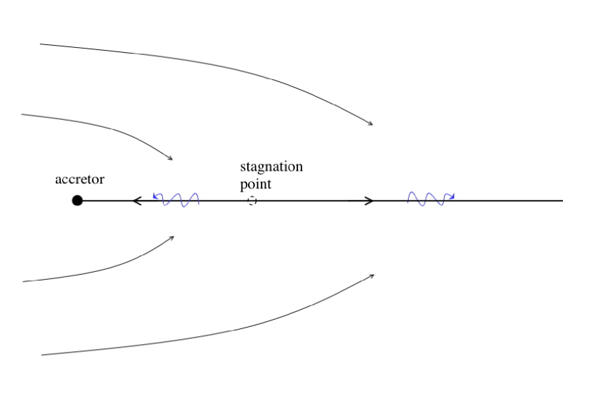
Figure 1: Schematic view of the accretion line model. Stream lines are drawn as solid lines with arrows. When pressure is taken into account (Sect. 3.2), density perturbations in the accretion line propagate as acoustic waves (wavy lines with arrows).

The region of the stagnation point is necessarily subsonic, and longitudinal pressure forces cannot be neglected there. Pressure forces in the stationary accretion line were considered by Wolfson (1977), Yabushita (1978a) and Horedt (2000). The simplest formulation corresponds to the isothermal hypothesis, in which the dynamical equations (1-2) are changed into:

$${\partial\rho\over\partial t}+{\partial\rho v\over\partial r} = H(r),$$ (6)

$${\partial v\over\partial t}+v{\partial v\over\partial r} = F(r,\rho,v)-{c^{2}\over\rho}{\partial\rho\over\partial r},$$ (7)

where $c$ is the isothermal sound speed. Again, a single differential equation is obtained for the radial structure of the linear perturbation $h$ of the mass flux (Eq. (58)), describing the propagation of acoustic waves modified by the external forces $F$. The solution is approximated at high frequency through a WKB analysis, away from the sonic points ($v=\pm c$):

$$h\sim\rho^{1\over 2}\exp\int{{\rm d}r\over v\pm c}\left[i\omega+{1\over 2}\left({\partial F\over\partial v}\pm{\rho\over c}{\partial F\over\partial\rho}\right)\right],$$

$${\rm for}\;\;\omega\gg{\rho v\over c^{2}}{\partial F\over\partial\rho}.$$ (8)

This stability analysis resembles that of radiation driven winds, studied by Mestel, Moore & Perry (1976) and Mathews (1976). Considering a uniform gravitational acceleration $g$ and a linearized radiative force ($F\equiv A\rho-g$, $H\equiv 0$), they showed that acoustic waves propagating outwards are amplified by radiation. In addition to the density effect $\partial F/\partial\rho$, the velocity effect $\partial F/\partial v$ is formally well known in line-driven winds (see e.g. Carlberg 1980, and more recent reviews by Owocki 1994, Feldmeier & Owocki 1998). $\partial F/\partial v<0$ in the accretion line model, implying that this velocity effect is always stabilizing, independently of the direction of propagation. This could have been anticipated directly from the Euler equation, since a positive perturbation of velocity results in a decreased external force. By contrast, the effect of the density dependence (term $\partial F/\partial\rho$) is opposite for outgoing and ingoing waves:

$${\partial F\over\partial v}\pm{\rho\over c}{\partial F\over\partial\rho} = -{v\over r-\alpha}\left(1\pm{v_{\infty}-v\over c}\right)\;\;{\rm in\;3D},$$ (9)

$$= -{v\over r^{1\over 2}(r^{1\over 2}-\alpha)}\left(1\pm{v_{\infty}-v\over c}\right)\;\;{\rm in\;2D}.$$ (10)

The density effect $\partial F/\partial\rho<0$ is thus stabilizing for waves propagating outwards and destabilizing for waves propagating inwards. This can be understood as follows: with $\partial F/\partial\rho<0$, a positive density perturbation is associated with a decreased external force. According to the Euler equation, this decreased force has a damping effect on the positive velocity perturbation associated with a wave propagating outwards, whereas it amplifies the negative velocity perturbation associated with a wave propagating inwards. In contrast with the instability without pressure found by Cowie (1977), this possible amplification of ingoing acoustic waves is not oscillatory. Altogether, the density and velocity effects damp outgoing acoustic waves. According to Eqs. (8) and (9-10), acoustic waves propagating inwards may be amplified only if

$$c+v<v_{\infty}.$$ (11)

This condition cannot be fulfilled far from the accretor since $v\sim v_{\infty}$ for $r\gg\alpha$. From this we conclude that the only possible amplification of high frequency acoustic waves is restricted to ingoing waves in a region of finite size. The size of this region is independent of frequency. The amplification factor ${\cal A}$, deduced from the WKB analysis, is also independent of the perturbation as long as its frequency is high enough to satisfy Eq. (8). It can be estimated as follows in 3D:

$${\cal A} \sim \exp\int{v_{\infty}-v-c\over 2c}{v\over r-\alpha}{{\rm d}r\over v-c}\;\;{\rm for}\;\;\omega\gg{v^{2}\over c^{2}}{v_{\infty}-v\over r-\alpha}.$$ (12)

$$\leq {\rm e}^{{\cal M}_{\infty}}$$ (13)

This contrasts with the instability found by Cowie (1977) which could be arbitrarily fast at high frequency (Eqs. 4-5).

3.3 The longitudinal instability beyond the accretion line model

The longitudinal instability of the accretion line proves that if the Mach number is high enough, the amplification of ingoing acoustic waves should be visible in numerical simulations. Such a transient amplification, however, cannot be considered to be a convincing mechanism to explain the instability observed in numerical simulations for moderate Mach numbers ${\cal M}_{\infty}\sim 3-5$. A true instability would require a feedback loop, in order to build an acoustic cycle. Ingoing acoustic waves may be partially reflected outwards near the accretor. Outgoing waves, however, are likely to escape to infinity rather than be reflected inwards again. Moreover, their amplitude is damped by the effect of the accreted momentum. In conclusion, the longitudinal instability of the accretion line does not explain the instability of BHL accretion.

4 A new look at the transverse instability of the accretion line

4.1 High frequency approximation of the transverse instability

Soker (1990) extended the stability analysis of Cowie (1977) to the case of transverse perturbations in 2D planar flows. The position of the accretion line is described in polar coordinates $\theta=\Theta(r)$. The angle $\Psi$ between the tangent to the accretion line and the symmetry axis, and the transverse velocity $v_{\theta}$ are related to $\Theta$ as follows:

$$\Psi=\Theta+r{\partial\Theta\over\partial r},$$ (14)

$$v_{\theta}=r\left({\partial\over\partial t}+v{\partial\over\partial r}\right)\Theta.$$ (15)

As remarked by Soker (1990), the transverse instability is decoupled from the longitudinal one. The angle $\Theta$ of the accretion line satisfies a second order differential equation, which is approximated at high frequency in Appendix D using a WKB analysis:

$$\Theta \propto {1\over r^{5\over 4}}\exp\left[i\omega r\pm 2^{1\over 2}(1+i)\omega^{1\over 2}r^{1\over 2}\right]\;\;{\rm for}\;\;r\gg\alpha,$$ (16)

$$\Theta \propto {1\over r^{7\over 8}}\exp\left[i\omega\int{{\rm d}r\over v}\pm{2(1-i)\over 5\alpha^{1\over 2}}\omega^{1\over 2}r^{5\over 4}\right]\;\;{\rm for}\;\;r\ll\alpha.$$ (17)

According to Eq. (16), the larger the distance from the accretor, the larger the amplification of perturbations. As for the longitudinal instability, the amplification in the region of accretion ceases close to the accretor at $r\propto\omega^{-2/5}$, and thus depends on the numerical resolution. These high frequency estimates could be used to compare the radial profiles of the transverse and longitudinal instabilities of the accretion line in the linear regime in 2D flows: the differences between Eqs. (16-17) and Eqs. (53-54) are not significant on the scale of few accretion radii, and cannot be responsible for the dominant longitudinal instability observed in the non linear simulations of Soker (1991).

4.2 Comparison of the transverse instability with the instability of a flag

More generally, a system satisfying a transverse equation of the form

$$\left({\partial\over\partial t}+v{\partial\over\partial r}\right)v_{\theta}=A\Theta+B\Psi+Cv_{\theta},$$ (18)

with arbitrary coefficients $A,B,C$, is unstable at high frequency. The differential equation (63) satisfied by $\Theta$ is written in Appendix D. If $v\neq 0$, the WKB approximation at high frequency is as follows:

$$\Theta\propto\left({v\over r^{2}B}\right)^{1\over 4}\exp\int\left[{i\omega\over v}+{C\over 2v}+{B\over 2v^{2}}\pm\left({i\omega B\over v^{3}}\right)^{1\over 2}\right]{\rm d}r,$$

$${\rm for}\;\;\omega\gg{v\over r},C,{Av\over rB},{\partial\log\over\partial r}{B\over v^{2}}.$$ (19)

This formulation outlines the role of the restoring force $B\Psi$ in driving the high frequency instability. $B\equiv-1/(r^{1\over 2}\rho)$ in the 2D accretion line model. This mechanism is reminiscent of the instability of a flag as described by Argentina et al. (2004), where the hydrodynamical force acting on the flag is also proportional to the inclination $\Psi$. The equation describing the transverse motion of a flag with infinite flexibility corresponds to the same Eq. (18), with $v\equiv 0$, $A\equiv 0$, $B\equiv-\alpha U_{0}$ and $C\equiv\alpha$, where $U_{0}$ is the wind velocity and the coefficient $\alpha>0$ characterizes the aerodynamic force acting on the flag. The solution of Eq. (18) when $v\equiv 0$ is unstable at high frequency if $B<0$:

$$\Theta\propto{1\over r}\exp\int\left[i\omega{C\over B}-{\omega^{2}\over B}-{A\over rB}\right]{\rm d}r.$$ (20)

The presence of finite flexibility (”flexural rigidity”) in a realistic flag material would set an upper bound to unstable frequencies. The comparison with the instability of a flag suggests the possible existence of a transverse instability of the subsonic region of the stagnation point ($v\sim 0$).

4.3 The transverse instability beyond the accretion line model

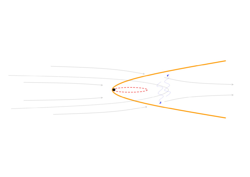
Figure 2: Transverse instability growing in the vicinity of the stagnation point. The shock (thick line), the sonic surface (dashed line) and the stream lines (thin lines with arrows) are drawn. The thin dotted line delineates the accreted gas. The transverse motion of the shock on one side is transmitted to the other side through acoustic waves (wavy lines with arrows).

4.3.1 Transient growth of the transverse instability in a shock cone

The accretion line model relies on the asumption that the half angle $\theta_{0}$ of the shock cone is small compared to other distances. Identifying the shock cone with the Mach cone, $\theta_{0}\sim 1/{\cal M}_{\infty}$ is indeed small if the incident flow is highly supersonic. With a longitudinal wavelength comparable to $\sim 2\pi v/\omega$, the transverse instability of the accretion line model is valid only for

$${2\pi v\over\omega}\gg{2r\over{\cal M}_{\infty}}.$$ (21)

The maximum exponential amplification ${\cal A}$ deduced from Eqs. (16-17) is thus bounded by:

$${\cal A}\leq\exp(2\pi{\cal M}_{\infty})^{1\over 2}.$$ (22)

Taking into account the finite width of the shock cone sets an upper bound $\propto{\cal M}_{\infty}$ to the frequency of the most unstable perturbations in a plane 2D flow. An additional limitation to the accretion line model comes from the acoustic time across the shock cone, which is a lower bound to the growth time of the instability. This also favours the subsonic region surrounding the stagnation point rather than the supersonic regions away from it. The instability as described by Soker (1990) is a local mechanism, taking place in the advected flow. A global mode as observed in the 2D plane simulations of the flip-flop instability requires an acoustic feedback inside the subsonic region. This instability could be described as a purely acoustic cycle between the opposite sides of the shock cone as in Fig. 2.

4.3.2 Towards a global transverse instability in BHL accretion ?

The amplification of transverse perturbations should be visible if the Mach number is high enough. Whether this is sufficient to explain the instability observed in 2D flows at low Mach number is not clear since this instability is transient. When pressure is taken into account, the region of the stagnation point seems to be a privileged place for the growth of a global mode involving transverse displacement and acoustic propagation.
The fate of the transverse instability in 3D BHL accretion is rather uncertain, as remarked by Soker (1991). Obviously transverse motions of the accretion line are forbidden in 3D, since incoming symmetrical trajectories which do not intersect the displaced accretion line meet along the symmetry axis and generate a new accretion line. This does not exclude a possible unstable oscillation of the shock cone in a transverse direction, such that the symmetry axis stays inside the accretion shock. According to Eqs. (18-19), the existence of a transverse restoring force proportional to the inclination angle is enough to generate a high frequency instability. Beyond geometrical factors, this force is still present in the 3D geometry. This instability mechanism could thus be present for high enough Mach numbers, although it has never been observed clearly in 3D numerical simulations. A correct description of the stability with respect to transverse oscillations would require taking into account pressure effects and the 3D dynamical deformation of the shock cone, which is much more difficult than the accretion line formalism.

5 The advective-acoustic mechanism in BHL accretion

5.1 Schematic formulation of a global cycle

The advective-acoustic instability deals with the cycle of advected perturbations (entropy, vorticity) coupled to acoustic waves, between the shock and the sonic surfaces. The coupling at the shock is a local process associated to the conservation laws through the shock. By contrast, the coupling due to the inhomogeneity of the subsonic flow occurs all the way from the shock to the sonic surface. F01 showed in a simple radial geometry that this acoustic feedback is described by an integral over the subsonic region, dominated by the region close to the sonic point, where the temperature is highest. This allows us to decompose the advective-acoustic cycle in four steps as follows:

(1) advection of an entropy/vorticity perturbation from the shock to the sonic point,

(2) excitation of an acoustic feedback due to the inhomogeneity of the flow,

(3) propagation of this acoustic feedback towards the shock,

(4) excitation of a new entropy/vorticity perturbation on the shock surface.
Each of these steps $j=1$ to $4$ is characterized by an efficiency ${\cal Q}_{j}$ measuring the amplification of perturbations. This decomposition is motivated by the existence of invariants, allowing a direct calculation of ${\cal Q}_{1}$ based on the conservation of entropy, or ${\cal Q}_{3}$ based on the conservation of acoustic energy. The stability of the global cycle depends on the product ${\cal Q}$:

$${\cal Q}\equiv{\cal Q}_{1}\times{\cal Q}_{2}\times{\cal Q}_{3}\times{\cal Q}_{4}$$ (23)

The linear growth rate of the advective-acoustic cycle, measured by the imaginary part of the eigenfrequency $\omega\equiv(\omega_{r},\omega_{i})$, can then be approximated by

$$\omega_{i}\sim{1\over\tau}\log|{\cal Q}|,$$ (24)

where $\tau$ is the duration of the advective-acoustic cycle, generally dominated by the advection time. Note that this schematized approach neglects the purely acoustic cycle, which can influence the stability threshold (FT00, F02).

5.2 Efficiencies ${\cal Q}_{i}$ based on radial accretion

In a radial flow with $\gamma>1$, we choose to measure, in the entropic-acoustic cycle, the amplification of the perturbation $f$ of the Bernoulli constant :

$$f\equiv v\delta v+{2\over\gamma-1}c\delta c.$$ (25)

Let us denote by $f^{\pm}$ its values for pressure perturbations $\delta p^{\pm}$ corresponding to an energy flux $F^{\pm}$ propagating with $(+)$ or against ($-$) the stream, and $f^{S}$ for entropy perturbations $\delta S$. At high frequency, for low degree waves $l=0,1,2$:

$$F^{\pm} \propto {1\over{\cal M}c^{2}}|f^{\pm}|^{2},$$ (26)

$$f^{\pm} \sim (1\pm{\cal M})c^{2}{\delta p^{\pm}\over\gamma p},$$ (27)

$$f_{S} \sim {c^{2}\over\gamma}\delta S.$$ (28)

Non radial entropy perturbations $\delta S$ are associated to vorticity perturbations $\delta w$ in shocked spherical accretion through Eqs. (80) to (82), so that the amplification of the entropy $\delta S\rightarrow\delta p^{-}\rightarrow\delta S^{\prime}$ also measures the simultaneous amplification of vorticity $\delta w\rightarrow\delta p^{-}\rightarrow\delta w^{\prime}$. In the isothermal limit ($\gamma\rightarrow 1$), vorticity is more appropriate than entropy to describe the advective-acoustic cycle, which becomes a vortical-acoustic cycle (F02) .

The steps (1) and (3) of advection and propagation in the spherical accretion flow studied by F01, F02 are deduced from Eqs. (26) and (28) and the conservations of entropy $\delta S$ and acoustic energy $F^{-}$:

$${\cal Q}_{1} \equiv {f_{\rm son}^{S}\over f_{\rm sh}^{S}}\sim{c_{\rm son}^{2}\over c_{\rm sh}^{2}}\;\;{\rm for}\;\;\omega_{r}\sim{c_{\rm son}\over r_{\rm son}},$$ (29)

$${\cal Q}_{3} \equiv {f_{\rm sh}^{-}\over f_{\rm son}^{-}}\sim{\cal M}_{\rm sh}^{1\over 2}{c_{\rm sh}\over c_{\rm son}},$$ (30)

where the subscripts ”son” and ”sh” refer to the sonic point and the shock respectively. Although the acoustic energy is conserved, the amplitude of outgoing waves $f^{-}$ decreases (${\cal Q}_{3}<1$) due to the geometric dilution in a diverging flow.
The advection of an entropy perturbation in a hot region may greatly increase the thermal energy carried by this perturbation, by a factor comparable to the temperature ratio (Eq. (29)). As sketched by FT00, the difference of energy is carried away by acoustic waves, propagating both upward and downward. Even the waves propagating downward may be refracted upward at low enough frequency (F01). The ratio ${f_{\rm son}^{-}/f_{\rm son}^{S}}$ is thus of order unity:

$${\cal Q}_{2}\equiv{f_{\rm son}^{-}\over f_{\rm son}^{S}}\sim 1.$$ (31)

The advective-acoustic coupling ${\cal Q}_{4}$ at the shock is deduced from a local analysis of a perturbed shock, performed in Appendix F:

$${\cal Q}_{4}\equiv{f_{\rm sh}^{S}\over f_{\rm sh}^{-}}\propto{1-{\cal M}_{\rm sh}\over{\cal M}_{\rm sh}}.$$ (32)

This equation is identical to Eqs. (16) and (C.11) in FT00, obtained for radial perturbations. ${\cal Q}_{4}$ may reach large values in nearly isothermal flows with strong shocks (${\cal M}_{\rm sh}\sim 1/{\cal M}_{1}$), in which case the dominant advected perturbations are non radial (F02): this is the basis of the vortical-acoustic cycle. The factor $(1-{\cal M}_{\rm sh})$ in Eq. (32) is responsible for the damping of the advective-acoustic coupling for weak shocks.
Altogether,

$${\cal Q}\propto{c_{\rm son}\over c_{\rm sh}}{1-{\cal M}_{\rm sh}\over{\cal M}_{\rm sh}^{1\over 2}}.$$ (33)

This approximate formula illustrates the two regimes of efficient advective-acoustic coupling identified by FT00, F01, F02:

(i) Strong temperature gradients are responsible for an efficient triggering of acoustic waves from advected entropy perturbations, which is the basis of the entropic-acoustic cycle (FT00, F01).

(ii) Strong entropy/vorticity perturbations can be produced at the shock if the post shock Mach number ${\cal M}_{\rm sh}$ is small.
These two sources of amplification can be used as guidelines for anticipating the properties of advective-acoustic cycles in BHL accretion flows. However, the dependence of ${\cal Q}$ on the frequency and the degree $l$ of the perturbation requires further calculations. In particular, F01 showed that the acoustic feedback is strongest for non radial modes $l=1$. Note also that Eq. (33) is singular if $c_{\rm son}\to\infty$ as is the case for 3D accretion with $\gamma=5/3$, which deserves a more careful analysis (Appendix G).

5.3 From radial to BHL accretion

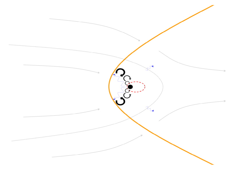
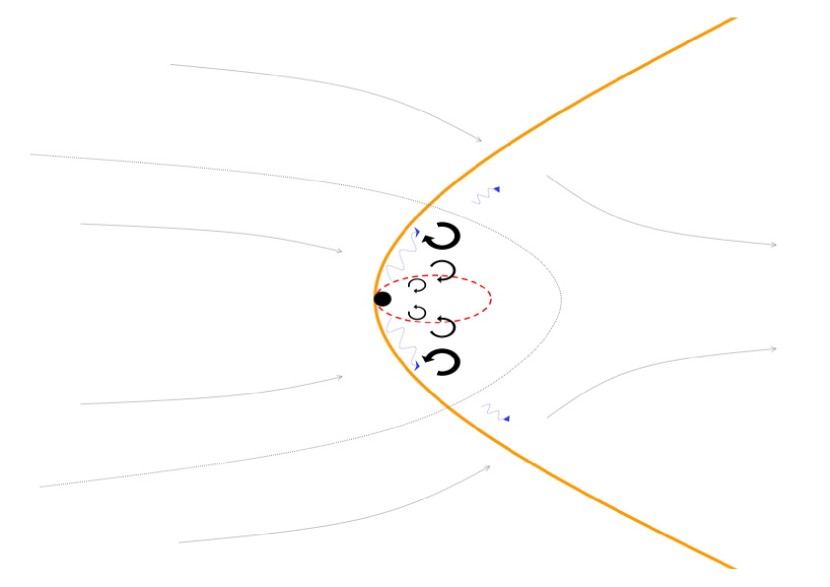
Figure 3: Schematic view of a global mode if the shock is detached or attached. Drawn lines have the same meaning as in Fig. 2. Perturbations of entropy/vorticity (circular arrows) follow the flow lines from the shock to the accretor, producing an acoustic feedback which propagates to the shock. A fraction of the acoustic energy may leak outside of the accretion cylinder.

5.3.1 Extrapolation to detached shocks

The locus of the advective-acoustic cycle is different if the shock is attached or detached (Fig. 3). A global mode between a bow shock and the accretor resembles the advective-acoustic cycle in a shocked radial flow. In this case the efficiency of the advective-acoustic cycle can be estimated from the study of radial accretion. By contrast, if the shock is attached to the accretor, most of the flow is accreted from behind in a supersonic manner. The value of ${\cal Q}_{2}$ in this particular geometry cannot be directlly extrapolated from its value in a radial flow.

5.3.2 Geometrical factors

In BHL accretion, the shape of the shock surface is not only non-spherical but open to infinity. The value of ${\cal Q}_{3}$ might be reduced by a geometrical factor $\sim 2$ compared to spherical accretion because a significant fraction of acoustic waves may propagate away from the region of accretion and leave the cycle (Fig. 3).
Conversely, the value of ${\cal Q}_{1}$ should be increased by the amplification of vorticity perturbations through the local KH and RT mechanisms (FR99), due to vorticity and entropy gradients in the post-shock flow.
The efficiencies ${\cal Q}_{i}$ estimated in spherical geometry should thus be considered, at best, as very rough approximations of those in the BHL flow.

5.4 Influence of the parameters $\gamma$, ${\cal M}_{\infty}$ and $r_{*}$

According to FT00, F01, the stability of the entropic-acoustic cycle depends essentially on the temperature increase between the shock and the sonic point. The most unstable cycle involves high frequency acoustic waves, those able to explore the hottest parts of the flow but still be refracted out, with a wavelength slightly larger than the smallest size of the sonic surface. Using the Bernoulli equation, the temperature on a point of the sonic surface is directly related to its distance $r_{\rm son}$ to the accretor:

$$c_{\rm son}^{2}={\gamma-1\over\gamma+1}\left[{2GM\over r_{\rm son}}+c_{\infty}^{2}\left({\cal M}_{\infty}^{2}+{2\over\gamma-1}\right)\right].$$ (34)

The closer the sonic surface to the accretor, the higher the temperature, and the more efficient the entropic-acoustic cycle. The calculation of Appendix A indicates that the sonic surface is always attached to the accretor if $\gamma=\gamma_{\rm max}$, with

$$\gamma_{\rm max} \equiv 3\;\;{\rm in\;2D},$$ (35)

$$\gamma_{\rm max} \equiv {5\over 3}\;\;{\rm in\;3D},$$ (36)

even if the shock is detached. Fig. 17 of R94 shows the shape of the attached sonic surface for 3D accretion with $\gamma=5/3$. Together with Eq. (33), the strength $\cal Q$ of the instability should increase when $\gamma$ approaches $\gamma_{\rm max}$ and $r_{*}$ decreases. The strength of the instability should be asymptotically independent of the incident Mach number for strong shocks. Conversely, the instability should be suppressed if the shock is weak (${\cal M}_{\rm sh}\sim 1$).
According to Appendix A, a critical index $\gamma_{\rm crit}<\gamma_{\rm max}$ must exist, below which the shock is always attached to the accretor, whatever its size. Numerical simulations with $\gamma=4/3$ (R95) suggest that $\gamma_{\rm crit}<4/3$ in 3D flows. The entropic-acoustic cycle is expected to be an efficient instability mechanism in the range $[\gamma_{\rm crit},\gamma_{\rm max}]$, as long as the distance of the sonic surface is small enough.
Nearly isothermal flows ($\gamma\sim 1$) could be unstable through the vortical-acoustic cycle, fed by ${\cal Q}_{4}\gg 1$ for strong shocks. However, the effect of the acoustic feedback in the particular geometry of an attached shock is uncertain. Neither the vortical-acoustic mechanism nor the extrapolated transverse instability manage to explain why isothermal BHL accretion seems so much more unstable in planar flows (SMA98) than in 3D simulations (R96).

6 Can the different numerical simulations be reconciled?

6.1 Some simulations are stable

The stability of the 2D planar flow simulated by FI98b, FI99, with a relativistic accretor contrasts with the many unstable simulations performed in Newtonian gravity. This is by no mean a relativistic stabilization of BHL accretion through relativistic effect, as recognized by FI98b. Indeed, they restricted their studies to $v_{\infty}/c_{\rm light}=0.5$, which corresponds to a rather big Schwarzschild radius in units of the accretion radius: $r_{\rm Sch}/r_{\rm A}=0.25$. These flows would have been stable even in the Newtonian limit.
According to ZWN95, the flow simulated by MSS91 becomes stable if the square accretor is replaced by a polygon. Although the shape of the accretor may influence the instability threshold, the existence of strongly unstable simulations in polar coordinates (BLT97 and SMA98) shows that 2D accretion can be unstable even if the accretor is perfectly spherical. The smaller accretor size and higher resolution used by BLT97 and SMA98, compared to ZWN95 (see Table 1), may be a hint in favour of an advective-acoustic mechanism. A direct comparison, however, is hampered by the fact that the adiabatic indices are different in these three simulations. The influence of the shape of the accretor, demonstrated by ZWN95, speaks against the transverse acoustic instability. These rather indirect arguments, if not conclusive, show at least that it is possible to reconcile existing simulations of 2D plane accretion in the framework of the advective-acoustic mechanism.

The stable 3D simulations can also be analyzed in the framework of the entropic-acoustic cycle. This cycle is stabilized by a weak shock, and destabilized by a small accretor size.

-Table 1 indicates that most axisymmetric simulations of an absorbing accretor are stable (SMT85, PSS89, SMA89), with the exception of KMS91 which shows an instability when $r_{*}/r_{\rm A}\leq 0.05$ and ${\cal M}\geq 2.4$. The existence of a threshold for the accretor size and the minimum Mach number fits perfectly with the entropic-acoustic mechanism.

-In the axisymmetric simulations of FI98a with $v_{\infty}/c_{\rm light}=0.5$, the Schwarzschild radius is too big to allow for a detached shock. According to Newtonian 3D simulations, the shock distance scales like a fraction (e.g. typically $0.2-0.4$ in R94) of the accretion radius. A slower black hole would have a detached shock, and the entropic-acoustic instability could develop naturally if the temperature gradient is sufficient. The shock gets detached in the simulation of FI98a for $\gamma=5/3$, $v_{\infty}/c=0.15$, but the shock is then too weak (${\cal M}_{\infty}=1.5$) to be destabilized. Indeed, the Newtonian simulations of Ruffert with ${\cal M}_{\infty}=1.4$ were also stable. A decisive test could be made by simulating an axisymmetric flow with $\gamma=5/3$, ${\cal M}_{\infty}=3$, and $v_{\infty}/c\leq 0.1$.

-The apparent stability observed in the simulations of POM00, in particular for $\gamma=5/3$, cannot be explained by simple considerations about the accretor size and shock strength. This result may be attributed to the particular numerical method of local time step used by the authors. In Sect. 3 of POM00, the authors make the following statement: ”It is important to note from the very begining that we seek steady state solution and generally do not perform time-accurate calculations (local time step inside each cell for the sake of computational efficiency)”. This method might not be adequate to propagate high frequency acoustic waves across the subsonic region.

6.2 Numerical artefacts in the simulations

Numerical issues are numerous. Besides the damping effect of numerical viscosity (SPH and Eulerian codes were compared by BA94) and the possible axis effect in axisymmetric simulations (FTM87), more subtle effects can be understood through the advective-acoustic cycle. This instability mechanism is physical, but may be artificially triggered or damped by numerical effects such as the carbuncle phenomenon at the shock, the boundary condition at the surface of the accretor and the grid size in between. The accuracy of both the advection of entropy/vorticity perturbations and the propagation of acoustic waves, between the shock and the sonic surface, is crucial for advective-acoustic instabilities.

6.2.1 Carbuncle phenomenon at the shock

POM00 drew attention to possible numerical instabilities at the shock in the BHL flow. In the region where the shock is parallel to the grid, the carbuncle instability (e.g. Robinet et al. 2000) may favour the generation of vorticity and entropy perturbations, which in turn can feed an advective-acoustic cycle. Conversely, one should carefully check the effect of any numerical procedure designed to damp the carbuncle instability at the shock, since it may also damp the coupling between advected and acoustic perturbations.

6.2.2 Grid resolution between the shock and the accretor

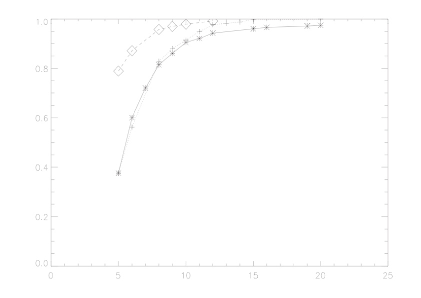
Figure 4: Numerical damping of a sinusoidal perturbation of entropy (full line) or vorticity (dotted line) advected over one wavelength, in a direction parallel to the grid, as a function of the number of grid points per wavelength. The flow is homogeneous with $\gamma=5/3$, and moves uniformly at Mach $0.2$. The dashed line corresponds to the damping of an acoustic wave propagated over one wavelength. In the three cases, the wavevector of the perturbation is parallel to the flow.

Vorticity is not usually computed with as much accuracy as momentum or energy in classical numerical schemes such as those used for BHL simulations. The artificial generation of vorticity at the interface of nested grids could feed a vortical-acoustic cycle.
Conversely, insufficient numerical resolution is responsible for an artificial damping of vorticity and entropy waves. As an example, Fig. 4 shows a measure of the damping of the amplitude of entropy and vorticity perturbations advected over one wavelength, in a direction parallel to the grid, as a function of the number of grid cells per wavelength. This test is performed on a Cartesian grid in 2D using the same PPM technique as in Ruffert (1994). The correct advection of entropy and vorticity in this numerical simulation requires as much as 10-15 grid cells per wavelength. Perturbations with a wavelength shorter than 10 grid cells are significantly damped over one wavelength. The same test performed on acoustic waves propagating over one wavelength shows a smaller damping: 5-10 grid cells are enough. This is a strong constraint for the correct calculation of an advective-acoustic cycle at high frequency which involves perturbations with a wavelength comparable to the accretor size, when the sonic surface is attached to it. The grid size should thus be at least 15-20 times smaller than the accretor size in order to properly describe the advective-acoustic coupling in the inner regions of the flow. This example illustrates the fact that the advective-acoustic instability can be impeded in a numerical simulation with insufficient resolution. Determining how these numbers depend on the numerical technique is beyond the scope of the present paper.

6.2.3 Boundary condition on the accretor

The size of the accretor is known to play an important role in the strength of the instability. One reason for this is that the sonic surface ahead of the accretor is generally attached to the accretor in numerical simulations. Boundary conditions at the surface of the accretor are therefore even more crucial, since they are in contact with a subsonic flow. The advection of entropy and vorticity perturbations through the boundary condition should be considered carefully in order to avoid an artificial acoustic feedback from the accretor. For example, imposing a transverse velocity equal to zero in the perturbed Bondi flow would generate a spurious feedback $f^{-}$ from any non spherical entropy/vorticity perturbations $f^{S}$, and artificially excite a vortical-acoustic cycle. A calculation in Appendix H of this condition at the boundary of a uniform, parallel flow shows that

$$\left({f^{-}\over f^{S}}\right)_{\rm boundary}=-1\;\;{\rm if}\;\;l\neq 0.$$ (37)

The artificial coupling due to inadequate boundary conditions can be as strong as the physical coupling ${\cal Q}_{2}$ expected from the temperature gradients in the flow.

6.3 Physical or numerical instability?

Many of the numerical artefacts discussed in Sect. 6.2 were not considered by the authors of the existing simulations. Could new simulations of BHL accretion, corrected from numerical artefacts, be stable? The physical arguments of Sect. 5 prove that the flow must be unstable, at least in the case $\gamma\sim 5/3$, ${\cal M}_{\infty}\geq 3$, for a small enough accretor: in this case, the efficiency ${\cal Q}$ of the entropic-acoustic cycle diverges when the accretor size $r_{*}\to 0$. Even the leak of acoustic energy cannot diminish the efficiency ${\cal Q}$ by more than a finite geometrical factor $2-3$, at most. The argument is weaker for $\gamma<5/3$, because ${\cal Q}$ depends strongly on the unknown shape of the sonic surface.

7 Future numerical tests of the instability mechanism

Future simulations should consider carefully the numerical artefacts listed in Sect. 6.2. The boundary condition at the surface of the accretor should be designed to absorb entropy and vorticity perturbations silently: this can be tested in a uniform flow. An alternative would be to find a set of parameters such that the accretor is fully embedded inside the sonic surface. Since $\gamma=5/3$ and $\gamma\sim 1$ are ruled out by FR97 in 3D, an intermediate choice could be $\gamma=4/3$ with ${\cal M}_{\infty}=3$, and a small enough accretor. The numerical issue of the absorbing boundary condition can also be solved naturally with general relativity, for any value of $\gamma$, since the flow is bound to be supersonic on the horizon of the black hole (FI98a,b).

The stable simulations analyzed in Sect. 6.1 call for new simulations which would directly test the efficiency of the advective-acoustic mechanism in accretion flows where the shock is detached:

-all the axisymmetric, Newtonian simulations with $\gamma=5/3$ should be unstable if ${\cal M}_{\infty}\geq 3$ and a small enough accretor ($r_{*}/r_{\rm A}\sim 0.005$ seems to be enough according to KMS91). In particular, new axisymmetric, relativistic simulations similiar to FI98a should become unstable when considering a slower accretor with a moderate shock, such as $v_{\infty}/c_{\rm light}=0.1$, $\gamma=5/3$, ${\cal M}_{\infty}=3$. The axisymmetric simulations of POM00 should also be unstable if their numerical technique allows for the advective-acoustic cycle.

-2D planar simulation should be unstable through the entropic-acoustic cycle if the shock is detached: comparing a simulation with $\gamma\sim 3$ (see Appendix A) and the classic flip-flop obtained for $\gamma\leq 5/3$ could help to understand the respective influences of the entropic-acoustic cycle and the purely acoustic transverse instability.

In an unstable simulation, the advective-acoustic mechanism could be tested directly by measuring the incoming entropy/vorticity perturbations and the outgoing acoustic flux in the subsonic region of the flow, as measured by Blondin et al. (2004) in his simulations of spherical accretion. An indirect way of testing the instability mechanism is to measure the effect of the various physical parameters. The linear growth rate of the entropic-acoustic cycle should increase when the accretor size is decreased, decrease for a weak shock and saturate for strong shocks. The present understanding of the 3D advective-acoustic instability when $\gamma\sim 5/3$ implies that its strength for an accretor size $r_{*}\sim 10^{-5}r_{\rm A}$ may be significantly under-estimated by the existing simulations ($r_{*}/r_{\rm A}>10^{-2}$). Tracing the power spectrum of the mass accretion rate (e.g. R95), as a function of the numerical resolution in the range accessible to computers, could give a hint on the extrapolation to smaller accretor sizes.

In order to better understand the instability of isothermal flows, it would be interesting to try to discriminate between a transverse instability (purely acoustic) and a vortical-acoustic cycle. The accretor size and boundary condition should play a more important role in a vortical-acoustic cycle than in a transverse instability.

8 Conclusion

The physical mechanisms underlying the longitudinal and transverse instabilities of the accretion line have been clarified. The destabilizing factor for the longitudinal instability is the density dependence of the external force per unit mass. The transverse instability is ruled by the restoring force proportional to the local inclination of the accretion line. The analogy with the instability of a flag has been outlined.
The overstable amplification of longitudinal high frequency perturbations of the accretion line found by Cowie (1977) is greatly affected by pressure forces. Density perturbations are propagated as acoustic waves. Those propagating outwards are damped, whereas those propagating inwards are transiently amplified. The analogy with the instability of radiation driven winds has been drawn.
The transverse instability of the accretion line is limited if the finite width of the shock cone is taken into account. A feedback process is necessary to explain the global flip-flop instability observed in planar 2D simulations. It seems possible that the mechanism of the transverse instability, modified by the propagation of acoustic waves within the subsonic region of the flow, leads to a global unstable mode. However, the influence of the shape of the accretor, demonstrated by ZWN95, may be a hint against this explanation of the instability.
For the first time, the advective-acoustic instabilitiy has been analyzed in the context of BHL accretion. This analysis is based on the extrapolation of the properties established in spherically symmetric flows (F01, F02). For this reason, the relevance of the advective-acoustic instabilities in BHL accretion is convincingly demonstrated only when the shock is detached from the accretor. The difference of geometry precludes an accurate prediction of the instability threshold in BHL accretion, especially since it is very sensitive to the size and shape of the sonic surface. Nevertheless, the analysis is predictive enough to assess that the advective-acoustic mechanism

- must be stable in the limit of a weak shock,

- must be unstable for 3D accretion flows with $\gamma\sim 5/3$, a reasonable shock strength ${\cal M}_{\infty}\geq 3$ and a small enough accretor size.
Numerical artefacts have also been discussed, specifically the grid size and the boundary conditions. We comment on how these artefacts must be circumvented to produce reliable numerical simulations of BHL accretion.
Surprisingly, it seems that all the existing numerical simulations can be reconciled in the framework of the advective-acoustic instability, with no striking contradiction, even when the shock is attached to the accretor. Several numerical tests of these ideas have been proposed.

Besides new numerical simulations, future analytic work ought to describe in more detail both the transverse instability modified by pressure forces, and the efficiency of the advective-acoustic cycle when the shock is attached. This could help understand why isothermal accretion is so much more unstable in 2D than in 3D.

Appendix A BHL stationary flow in 2D and 3D

A.1 Adiabatic index and pressure forces

The sonic radius in radial Bondi accretion, deduced from the Bernoulli equation and the conservation of mass flux, is different in 2D and 3D:

$$r_{\rm son} = {3-\gamma\over 2}{GM\over c_{\infty}^{2}}\;\;{\rm in\;2D},$$ (38)

$$r_{\rm son} = {5-3\gamma\over 4}{GM\over c_{\infty}^{2}}\;\;{\rm in\;3D}.$$ (39)

The existence of a sonic radius in radial accretion on a point like accretor requires $\gamma\leq 5/3$ in 3D, whereas plane supersonic accretion is possible up to $\gamma\leq 3$. This illustrates the fact that the 3D convergence of flow lines produces stronger pressure gradients than in 2D. These pressure gradients act against gravity. Extending to plane flows the argument used in FR97 for 3D flows, the sonic surface of a stationary BHL accretion must intersect the sphere of radius $r_{0}$ deduced from Eqs. (38-39), with

$$r_{0} \equiv {r_{\rm son}\over 1+{\gamma-1\over 2}{\cal M}_{\infty}^{2}}.$$ (40)

This suggests that the shock should be detached in planar accretion with $\gamma$ close to 3. SMA89 considered plane accretion with $\gamma=2$ but the shock was still not detached. The ratio $r_{0}/r_{\rm A}$ is a function of $\gamma,{\cal M}_{\infty}$:

$${r_{0}\over r_{\rm A}} = {3-\gamma\over 4}{{\cal M}_{\infty}^{2}\over 1+{\gamma-1\over 2}{\cal M}_{\infty}^{2}}\;\;{\rm in\;2D},$$ (41)

$${r_{0}\over r_{\rm A}} = {5-3\gamma\over 8}{{\cal M}_{\infty}^{2}\over 1+{\gamma-1\over 2}{\cal M}_{\infty}^{2}}\;\;{\rm in\;3D}.$$ (42)

As already noted in FR97, the sonic surface must also be attached to the accretor if $r_{0}/r_{\rm A}\geq 1$, because the sonic surface cannot extending beyond the distance $\sim r_{A}$ of the stagnation point. This concerns in particular isothermal flows with a strong shock, for which $r_{0}/r_{\rm A}\propto{\cal M}_{\infty}^{2}$. A critical index $\gamma_{\rm crit}$ must therefore exist, below which the shock is always attached to the accretor, whatever its size.

A.2 Accretion line

The mass flux per unit of length, along the accretion line, is constant in 3D whereas it varies like $r^{-{1\over 2}}$ for a planar flow (Soker 1990). By integrating Eq. (1) using Table 2,

$$\rho v = 2(r^{1\over 2}-\alpha^{1\over 2})\;\;{\rm in\;2D},$$ (43)

$$\rho v = r-\alpha\;\;{\rm in\;3D},$$ (44)

where $\alpha$ is the distance of the stagnation point. The asymptotic velocity within the accretion line, deduced from Eq. (2) for $r\gg\alpha$, is different in 2D and 3D:

$$v \sim 1-{\lambda\over r^{1\over 2}}\;\;{\rm in\;2D},$$ (45)

$$v \sim 1-{\log r\over r}\;\;{\rm in\;3D},$$ (46)

where $\lambda$ is a constant.

Appendix B Physical cause of the longitudinal instability of the accretion line

The growth rate computed by Cowie (1977) in 3D is the imaginary part of the complex frequency $\omega$:

$$(\omega-kv)^{2} = ik\left[v{{\rm d}v\over{\rm d}r}+{1\over 2r^{2}}\right].$$ (47)

The growth rate in 2D is given by strictly the same formula, although the accretion terms involve geometrical factors $1/r^{1\over 2}$ in Table 2. The absence of such factors in Eq. (47) led Soker (1990) to conclude that this instability is independant of accretion. This argument is insufficient, since Eq. (47) can be rewritten using the stationary flow equation Eqs. (2.7a-2.7b) of Soker (1990), as follows:

$$(\omega-kv)^{2} = {ik\over 2}{1-v\over\rho r^{1\over 2}}\;{\rm in\;2D},$$ (48)

$$= {ik\over 2}{1-v\over\rho}\;{\rm in\;3D}.$$ (49)

The geometrical factor $r^{1\over 2}$ is then clearly apparent. A closer look at the equations shows that the longitudinal instability is due to the density dependance of the force acting on the accretion line. Using the same normalizations of density, velocity and distances as in Soker (1990), the time dependent equations correspond to Eqs. (1-2).
A linearization of Eqs. (1-2) gives the differential equation satisfied by a perturbation of the mass flux $h\equiv\rho\delta v+v\delta\rho$:

$$v^{2}{\partial^{2}h\over\partial r^{2}}-{\partial h\over\partial r}\left\{2i\omega v-\rho{\partial\over\partial r}{v^{2}\over\rho}+v{\partial F\over\partial v}-\rho{\partial F\over\partial\rho}\right\}$$

$$-i\omega h\left\{\rho{\partial\over\partial r}{v\over\rho}-i\omega-{\partial F\over\partial v}\right\}=0.$$ (50)

The solution is written in Eq. (3) at high frequency $\omega$ using the WKB approximation. Contrary to the conclusions of Soker (1990), acceleration within the accretion line is not crucial for this instability. The simplest flow in which a similar instability occurs would be a flow with uniform density $\rho_{0}$ and velocity $v_{0}$, subject to a force depending linearly on density: $F\equiv a(\rho-\rho_{0})$ and without any mass accretion ($H\equiv 0$). The stationary flow being uniform, the uniform velocity could also be taken to be equal to zero owing to a simple change of reference frame. The evolution of perturbations can then be calculated precisely. The frequency $\omega$ and the wavevector $k$ are related through the following dispersion relation:

$$(\omega-kv_{0})^{2}=ik\rho_{0}{\partial F\over\partial\rho}$$ (51)

The growth rate corresponds to the imaginary part $\omega_{i}$:

$$\omega_{i}={a\rho_{0}\over 2(\omega_{r}-kv_{0})}$$ (52)

The amplification of perturbation is thus exponential in the direction of the external force for a positive enhancement of density. In the accretion line model, this amplification is weaker due to the weak density dependence of the external force. Using the asymptotic behaviour $v\propto-1/r^{1\over 2}$ close to the accretor, and Eq. (46) in 3D flows leads to Eqs. (4-5). By contrast, the same calculation using Eq. (45) in 2D flows leads to:

$$h(r)\propto r^{3\over 8}\exp\left[i\omega r\pm 2(1+i)\omega^{1\over 2}\lambda^{1\over 2}r^{1\over 4}\right],$$

$${\rm for}\;\;r\gg\alpha,$$ (53)

$$h(r)\propto r^{3\over 4}\exp\left[-{2\over 3}i\omega r^{3\over 2}\pm{1-i\over 2\alpha^{1\over 2}}\omega^{1\over 2}r\right],$$

$${\rm for}\;\;{1\over\omega^{1\over 2}}\ll r\ll\alpha.$$ (54)

The difference of asymptotic behaviors between the 2D and 3D cases is not significant.

Appendix C Effect of pressure forces on the longitudinal instability

The linearization of the perturbed flow leads to define the perturbation $f$ of the Bernoulliu constant as follows:

$$f \equiv v\delta v+c^{2}{\delta\rho\over\rho},$$ (55)

in order to obtain a simple second order differential system satisfied by $(f,g)$:

$$(c^{2}-v^{2}){\partial h\over\partial r} = i\omega\left(\rho f-vh\right),$$ (56)

$$(c^{2}-v^{2}){\partial f\over\partial r} = \left\{-i\omega v-v{\partial F\over\partial v}+\rho{\partial F\over\partial\rho}\right\}f$$ (57)

$$+\left\{\left(i\omega+{\partial F\over\partial v}\right)c^{2}-v\rho{\partial F\over\partial\rho}\right\}{h\over\rho}.$$

A single differential equation is obtained:

$$(c^{2}-v^{2}){\partial^{2}h\over\partial r^{2}}+{\partial h\over\partial r}\left\{2i\omega v+\rho{\partial\over\partial r}\left({c^{2}-v^{2}\over\rho}\right)\right.$$

$$\left.+v{\partial F\over\partial v}-\rho{\partial F\over\partial\rho}\right\}+i\omega h\left\{\rho{\partial\over\partial r}{v\over\rho}-i\omega-{\partial F\over\partial v}\right\}=0.$$ (58)

Before looking for approximate solutions to this equation, the effect of pressure forces can be easily incorporated in the simple toy model used in Appendix B, with uniform density and velocity:

$$\omega={i\over 2}{\partial F\over\partial v}+kv\pm\left[k^{2}c^{2}+ik\rho{\partial F\over\partial\rho}-{1\over 4}\left({\partial F\over\partial v}\right)^{2}\right]^{1\over 2}$$ (59)

The problem is formally identical to that idealized by Mestel, Moore & Perry (1976) and Mathews (1976), for radiation driven winds, where $F\equiv A\rho-g$. At high frequency:

$$\omega\sim k(v\pm c)+{i\over 2}\left({\partial F\over\partial v}\pm{\rho\over c}{\partial F\over\partial\rho}\right).$$ (60)

The stability of high frequency acoustic waves depends on the sign of the quantity between parenthesis. In a non uniform flow, a similar conclusion can be reached at high frequency through a WKB analysis, leading to Eq. (8).

Appendix D Transverse instability of the accretion line

The differential equation satisfied by $\Theta$ is:

$${\partial^{2}\Theta\over\partial r^{2}}+{\partial\Theta\over\partial r}\left\{{\partial\log r^{2}v\over\partial r}-{2i\omega\over v}+{1\over r^{1\over 2}v\rho}\left(1+{1\over v}\right)\right\}$$

$$-{\Theta\over r\rho v^{2}}\left\{r\rho\omega^{2}+2i\omega\rho v+i\omega r^{1\over 2}-{3\over 2r^{1\over 2}}\right\}=0.$$ (61)

The WKB approximation is thus:

$$\Theta\sim{(\rho v)^{1\over 4}\over r^{7\over 8}}\exp\int\left({i\omega\over v}-{1\over 2r^{1\over 2}v\rho}\right){\rm d}r$$

$$\exp\pm{1+i\over 2^{1\over 2}}\omega^{1\over 2}\int{{\rm d}r\over r^{1\over 4}\rho^{1\over 2}v^{3\over 2}},\;\;{\rm for}\;\;\omega\gg{3v\over 2r}.$$ (62)

The second order differential equation in the general case corresponding to Eq. (18) is:

$$v^{2}{\partial^{2}\Theta\over\partial r^{2}}+{\partial\Theta\over\partial r}\left({v\over r}{\partial rv\over\partial r}-2i{\omega v}-B-Cv\right)$$

$$+\Theta\left(-i\omega{v\over r}-{A+B\over r}+i\omega C-\omega^{2}\right)=0.$$ (63)

Appendix E Proof that $\delta K\equiv 0$ in the shocked Bondi flow

Let us recall the differential system satisfied by the perturbations $f,g$ defined in F01 (Eqs. (B18-B19)):

$$v{\partial f\over\partial r}+{i\omega{\cal M}^{2}f\over 1-{\cal M}^{2}} = {i\omega v^{2}g\over 1-{\cal M}^{2}}+i\omega c^{2}{\delta S\over\gamma},$$ (64)

$$v{\partial g\over\partial r}+{i\omega{\cal M}^{2}g\over 1-{\cal M}^{2}} = {i\omega f\over c^{2}(1-{\cal M}^{2})}-{iL^{2}\over\omega r^{2}}f+{i\delta K\over r^{2}\omega},$$ (65)

where the constant $\delta K$ and the function $\mu(r,\omega,l)$ are defined by:

$$\delta K \equiv r^{2}v\cdot(\nabla\times\delta w)+l(l+1)c^{2}{\delta S\over\gamma},$$ (66)

$$\mu^{2} \equiv 1-{l(l+1)\over\omega^{2}r^{2}}(c^{2}-v^{2}).$$ (67)

Consider a spherical adiabatic shock with incident Mach number ${\cal M}_{1}$ in the radial direction. Let this shock be perturbed by a sound wave with frequency $\omega$ propagating against the flow in the subsonic region, producing a displacement $\Delta\zeta(\theta,\varphi)$ and a perturbation $\Delta v(\theta,\varphi)$ of the radial velocity of the shock. Using the index ”1” before the shock, and ”2” after it, the conservation of mass flux and energy across the shock can be written as follows:

$$\rho_{1}(v_{1}-\Delta v) = \rho_{2}(v_{2}+\delta v_{2}-\Delta v),$$ (68)

$${(v_{1}-\Delta v)^{2}\over 2}+{c_{1}^{2}\over\gamma-1} = {(v_{2}+\delta v_{2}-\Delta v)^{2}\over 2}+{(c_{2}+\delta c_{2})^{2}\over\gamma-1},$$ (69)

where quantities are measured at the position ${r}_{\rm sh}+\Delta\zeta$. Keeping the first order terms, and using the defnition of $f,g$, together with the entropy equation, we obtain:

$$f = (v_{2}-v_{1})\Delta v,$$ (70)

$$g = \left({1\over v_{2}}-{1\over v_{1}}\right)\Delta v+\delta S.$$ (71)

A third equation relating $\delta S$ to $\Delta v,\Delta\zeta$ could be deduced using the conservation of impulsion, in the spirit of Nakayama (1994). A more direct derivation can be obtained by noting that entropy is conserved before and after the shock, and that the entropy jump across the shock depends only on the local value of the incident Mach number ${\cal M}_{1}^{\prime}$ in the frame of the shock (Eq. (72)):

$${\cal M}_{1}^{\prime}({r}_{\rm sh}+\Delta\zeta) = {\cal M}_{1}({r}_{\rm sh})+{\Delta v\over c_{1}}+\Delta\zeta{\partial{\cal M}_{1}\over\partial r},$$ (72)

$$= {\cal M}_{1}({r}_{\rm sh})+\left(1+{i\eta v_{2}\over\omega r}\right){\Delta v\over c_{1}},$$ (73)

$$\eta \equiv {\partial\log{\cal M}\over\partial\log r}$$ (74)

Using the Rankine-Hugoniot jump conditions, we obtain

$${\delta S}=-{4\gamma({\cal M}_{1}^{2}-1)^{2}\over(\gamma+1)^{2}{\cal M}_{1}^{2}}{c_{1}^{2}\over c_{2}^{2}}\left(1+{i\eta v_{2}\over\omega r}\right){\Delta v\over v_{1}}.$$ (75)

Equations (70-71) thus become:

$$f = -{2c_{1}^{2}\over\gamma+1}({\cal M}_{1}^{2}-1){\Delta v\over v_{1}},$$ (76)

$$g = {2\over\gamma+1}{c_{1}^{2}\over c_{2}^{2}}{{\cal M}_{1}^{2}-1\over{\cal M}_{1}^{2}}\left[1-{2\gamma\over\gamma+1}({\cal M}_{1}^{2}-1){i\eta v_{2}\over\omega r}\right]{\Delta v\over v_{1}}.$$ (77)

The perturbation of non radial velocity $\delta v_{\theta},\delta v_{\varphi}$ immediately after the shock is deduced from the conservation of the tangential component of the velocity across the shock, in the spirit of Landau & Lifschitz (1987).

$$\delta v_{\theta} = {v_{1}-v_{2}\over r}{\partial\Delta\zeta\over\partial\theta},$$ (78)

$$\delta v_{\varphi} = {v_{1}-v_{2}\over r\sin\theta}{\partial\Delta\zeta\over\partial\varphi}.$$ (79)

The vorticity immediately after the shock is deduced from the non radial component of the linearized Euler equations (B.11) and (B.12) of F01, together with Eq. (70) and Eqs (78-79):

$$w_{r} = 0,$$ (80)

$$w_{\theta} = -{c^{2}\over rv\sin\theta}{\partial\over\partial\varphi}{\delta S\over\gamma},$$ (81)

$$w_{\varphi} = {c^{2}\over rv}{\partial\over\partial\theta}{\delta S\over\gamma}.$$ (82)

Immediately after the shock, the constant $\delta K$ defined by Eq. (66) is computed using Eqs. (81) and (82):

$$\delta K=0.$$ (83)

Since $\delta K$ is conserved through the Bondi flow, $\delta K$ is uniformly equal to zero. As a consequence, using the integrated expression of the vorticity (Eqs. (B5) to (B7) in F01), the vorticity perturbation is described by Eqs. (80) to (82) throughout the flow.

Appendix F Advective-acoustic coupling at the shock

The perturbations $f,g$ after the shock are decomposed as follows:

$$f = f^{-}+f^{+}+f^{S},$$ (84)

$$g = g^{-}+g^{+}+g^{S},$$ (85)

where $f^{S},g^{S}$ correspond to the entropy/vorticity wave associated to the entropy perturbation $\delta S$ with $\delta K=0$, and $f^{\pm},g^{\pm}$ correspond to the purely acoustic waves propagating in the direction of the flow (index $+$) or against the flow (index $-$). Neglecting the coupling between the entropic and acoustic waves in the vicinity of the shock, the entropy wave $f^{S},g^{S}$ is advected at the velocity of the fluid:

$${\partial f^{S}\over\partial r} \sim {i\omega\over v}f^{S},$$ (86)

$${\partial g^{S}\over\partial r} \sim {i\omega\over v}g^{S}.$$ (87)

Replacing these derivatives in Eqs. (64-65), we obtain:

$$f^{S} \sim {1-{\cal M}_{2}^{2}\over 1-\mu^{2}{\cal M}_{2}^{2}}c^{2}{\delta S\over\gamma},$$ (88)

$$g^{S} \sim {\mu^{2}\over c^{2}}f^{S}.$$ (89)

Acoustic waves are described by Eqs. (64-65) in the absence of entropy perturbations, i.e. when $\delta S=0$. Using the WKB approximation of F01, the radial derivative of $f^{\pm}$ is approximated by:

$${\partial f^{\pm}\over\partial r}\sim{i\omega\over c}{{\cal M}\mp\mu\over 1-{\cal M}^{2}}f_{\pm}.$$ (90)

$g^{\pm}$ is deduced from Eqs. (64) and (90):

$$g^{\pm}\sim\pm{\mu\over{\cal M}c^{2}}f_{\pm}.$$ (91)

The linear system (84-85) can be transformed using Eqs.(88-89) and (91), in order to express the acoustic perturbations $f^{\pm}$:

$$f^{\pm}={1\over 2}\left[f\pm{{\cal M}\over\mu}c^{2}g-(1\pm\mu{\cal M})f^{S}\right].$$ (92)

Using this equation immediately after the shock, with Eqs. (75) to (77):

$$f^{\pm}\sim\mp{\gamma+1\over 4\gamma}{c^{2}\delta S\over 1-{\cal M}_{1}^{-2}}{{\cal M}_{2}\over\mu}\left({\mu^{2}\mp 2{\cal M}_{2}\mu+{\cal M}_{1}^{-2}\over 1\mp\mu{\cal M}_{2}}\right).$$ (93)

From Eqs. (88) and (93),

$${f^{S}\over f^{-}}={4\over\gamma+1}{\mu\over{\cal M}_{2}}{(1-{\cal M}_{2}^{2})(1-{\cal M}_{1}^{-2})\over(1-\mu{\cal M}_{2})(\mu^{2}+2\mu{\cal M}_{2}+{\cal M}_{1}^{-2})}.$$ (94)

At high frequency such that $\mu\sim 1$,

$${f^{S}\over f^{-}} = {4\over\gamma+1}{1+{\cal M}_{2}\over 1+2{\cal M}_{2}+{\cal M}_{1}^{-2}}{1-{\cal M}_{1}^{-2}\over{\cal M}_{2}},$$ (95)

$$\propto {1-{\cal M}_{2}\over{\cal M}_{2}}.$$ (96)

Appendix G Entropic-acoustic coupling in 3D for $\gamma\sim 5/3$

The value of $|{\cal Q}|$ deduced from F01 for $\gamma$ close to $5/3$ increases with frequency like $\omega_{r}^{1/3}$ (Eqs. 28-29 of F01), up to a maximum reached near the cut-off frequency. This behaviour can be understood in the framework of FT00, which argued that the efficiency of the entropic-acoustic coupling is related to the increase of enthalpy between the shock and the sonic point. A slight correction, however, should be made. Rather than the naive guess $|{\cal Q}|^{2}\propto c_{\rm son}^{2}/c_{\rm sh}^{2}$ of Eq. (23) in FT00, one must take into account the fact that the coupling of entropy perturbations to acoustic waves must occur before the sonic radius in order to allow significant outgoing acoustic flux. The effective radius of coupling $r_{\rm eff}$ was computed analytically in Appendix E of F01 (Eqs. E6 and E13):

$$r_{\rm eff} \propto \omega_{r}^{-{2\over 3}},$$ (97)

$$|{\cal Q}|^{2} \propto {c^{2}(r_{\rm eff})\over c^{2}(r_{\rm sh})}\propto\omega_{r}^{{2\over 3}}.$$ (98)

The efficiency ${\cal Q}^{2}$ deduced from the analytical calculations of F01 indeed scales like the ratio of enthalpies between the shock and the effective point of coupling $r_{\rm eff}$. The radius $r_{\rm eff}$ coincides with the wavelength $v/\omega_{\rm cut}$ of an entropy perturbation with a frequency $\omega_{r}$ close to $\omega_{\rm cut}$: the enthalpy effectively ”seen” by this perturbation is not the enthalpy at the sonic radius but rather at the effective radius $r_{\rm eff}$. From this point of view, using the same notations as in F01, $|{\cal Q}_{S}|_{l=1}\gg|{\cal Q}_{S}|_{l=0}$ is a natural consequence of $\omega_{1}^{\rm cut}\gg\omega_{0}^{\rm cut}$: non radial perturbations effectively ”see” regions of higher enthalpy. The most efficient entropic-acoustic coupling is reached at frequencies close to the refraction cut-off, where $\mu\sim 1$.

Appendix H Artificial acoustic feedback from the boundary condition on the accretor

The perturbed velocity in the direction perpendicular to the flow is deduced from the linearized Euler equations, using the vorticity given by Eqs. (81-82):

$$\delta v_{\theta} = {1\over i\omega r}{\partial f\over\partial\theta},$$ (99)

$$\delta v_{\varphi} = {1\over i\omega r\sin\theta}{\partial f\over\partial\varphi}.$$ (100)

A combination of these equations involves the eigenvalues of the Laplacian in spherical coordinates:

$$l(l+1)f = -{i\omega r\over{\rm sin}\theta}\left[{\partial\over\partial\theta}({\rm sin}\theta\delta v_{\theta})+{\partial\over\partial\phi}\delta v_{\phi}\right].$$ (101)

Imposing $\delta v_{\perp}=0$ on the boundary consequently requires $f=0$ there, if the perturbation is not spherically symmetric ($l\neq 0$). The acoustic feedback $f^{-}$ associated to the entropy/vorticity perturbation $f^{S}$ passing through the boundary condition $\delta v_{\perp}=0$, is deduced from the decomposition (84), with $f^{+}=0$ and $f=0$:

$$\left({f^{-}\over f^{S}}\right)_{\rm boundary} = -1\;\;{\rm if}\;\;l\neq 0.$$ (102)

References

- (1) Anzer, U., Börner, G., Monaghan, J.J. 1987, A&A 176, 235 (ABM87)
- (2) Argentina, M. & Mahadevan, L. 2004, arXiv:cond-mat/0402667
- (3) Benensohn, J.S., Lamb, D.Q., Taam, R.E. 1997, ApJ 478, 723 (BLT97)
- (4) Blondin, J.M., Kallman, T.R., Fryxell, B.A., Taam, R.E. 1990, ApJ 356, 591
- (5) Blondin, J.M, Mezzacappa, A., DeMarino, C. 2003, ApJ 584, 971
- (6) Boffin, H.M.J., Anzer, U. 1994, A&A 284, 1026 (BA94)
- (7) Bondi, H., Hoyle, F. 1944, MNRAS, 104, 273
- (8) Carlberg, R.G. 1980, ApJ 241, 1131
- (9) Cowie, L.L. 1977, MNRAS 180, 491
- (10) Edgar, R. 2004, New Astronomy Reviews 48, 843
- (11) Feldmeier, A., Owocki, S. 1998, Ap&SS 260, 113
- (12) Foglizzo, T. 2001, A&A 368, 311 (F01)
- (13) Foglizzo, T. 2002, A&A 392, 353 (F02)
- (14) Foglizzo, T., Ruffert, M. 1997, A&A 320, 342 (FR97)
- (15) Foglizzo, T., Ruffert, M. 1999, A&A 347, 901 (FR99)
- (16) Foglizzo, T., Tagger, M. 2000, A&A 363, 174 (FT00)
- (17) Font, J.A., Ibanez, J.M.A. 1998a, ApJ 494, 297 (FI98a)
- (18) Font, J.A., Ibanez, J.M.A. 1998b, MNRAS 298, 835 (FI98b)
- (19) Font, J.A., Ibanez, J.M.A., Papadopoulos, P. 1999, MNRAS 305, 920 (FIP99)
- (20) Fryxell, B.A., Taam, R.E. 1988, ApJ 335, 862 (FT88)
- (21) Fryxell, B.A., Taam, R.E., McMillan, S.L.W. 1987, ApJ 315, 536 (FTM87)
- (22) Horedt, G.P. 2000, ApJ 541, 821
- (23) Hoyle, F., Lyttleton, R.A. 1939, Proc. Cam. Phil. Soc., 35, 405
- (24) Hunt, R. 1971, MNRAS 154, 141 (H71)
- (25) Hunt, R. 1979, MNRAS 188, 83 (H79)
- (26) Ishii, T., Matsuda, T., Shima, E., Livio, M., Anzer, U., Börner, G. 1993, ApJ 404, 706 (IMS93)
- (27) Koide, H., Matsuda, T., Shima, E. 1991, MNRAS 252, 473 (KMS91)
- (28) Landau, L.D., Lifshitz, E.M. 1987, Fluid Mechanics, Vol. 6, Pergamon Press
- (29) Livio, M., Soker, N., de Kool, M., Savonije, G.J. 1986, MNRAS 222, 235 (LSK86)
- (30) Livio, M., Soker, N., Matsuda, T., Anzer, U. 1991, MNRAS 253, 633
- (31) Mathews, W.G. 1976, ApJ 207, 351
- (32) Matsuda, T., Inoue, M., Sawada, K. 1987, MNRAS 226, 785 (MIS87)
- (33) Matsuda, T., Ishii, T., Sekino, N., Sawada, K., Shima, E., Livio, M., Anzer, U. 1992, MNRAS 255, 183 (MIS92)
- (34) Matsuda, T., Sekino, N., Sawada, K., Shima, E., Livio, M., Anzer, U., Börner, G. 1991, A&A 248, 301 (MSS91)
- (35) Matsuda, T., Sekino, N., Shima, E., Sawada, K. 1989, MNRAS 236, 817 (MSS89)
- (36) Mestel, L., Moore, D.W., Perry, J.J. 1976, A&A 52, 203
- (37) Nakayama, K. 1994, MNRAS 270, 871
- (38) Owocki, S.P. 1994, Ap&SS 221, 3
- (39) Petrich, L.I., Shapiro, S.L., Stark, R.F., Teukolsky, S.A. 1989, ApJ 336, 313 (PSS89)
- (40) Pogorelov, N.V., Ohsugi, Y., Matsuda, T. 2000, MNRAS 313, 198 (POM00)
- (41) Robinet, J.C., Gressier, J., Casalis, G., Moschetta, J.M. 2000, J. Fluid Mech. 417, 237
- (42) Ruffert, M. 1994, A&AS 106, 505 (R94)
- (43) Ruffert, M. 1995, A&AS 113, 133 (R95)
- (44) Ruffert, M. 1996, A&A 311, 817 (R96)
- (45) Ruffert, M. 1997, A&A 317, 793 (R97)
- (46) Ruffert, M. 1999, A&A 346, 861 (R99)
- (47) Ruffert, M., Anzer U. 1995, A&A 295, 108
- (48) Ruffert, M., Arnett D. 1994, ApJ 427, 351 (RA94)
- (49) Sawada, K., Matsuda, T., Anzer, U., Börner, G., Livio, M. 1989, A&A 221, 263 (SMA89)
- (50) Shima, E., Matsuda, T., Anzer, U., Börner, G., Boffin, H.M.J. 1998, A&A 337, 311 (SMA98)
- (51) Shima, E., Matsuda, T., Takeda, H., Sawada, K. 1985, MNRAS 217, 367 (SMT85)
- (52) Soker, N. 1990, ApJ 358, 545
- (53) Soker, N. 1991, ApJ 376, 750
- (54) Soker, N., Livio, M., de Kool, M., Savonije, G.J. 1986, MNRAS 221, 445 (SLK86)
- (55) Taam, R.E., Fryxell, B.A. 1989, ApJ 339, 297 (TF89)
- (56) Taam, R.E., Fu, A., Fryxell, B.A. 1991, ApJ 371, 696
- (57) Wolfson, R. 1977, ApJ 213, 200
- (58) Yabushita, S. 1978, MNRAS 182, 371
- (59) Zarinelli, A., Walder, R., Nussbaumer, H. 1995, A&A 301, 922 (ZWN95)