Particle Swarm Optimization: An efficient method for tracing periodic orbits in 3D galactic potentials

Abstract

We propose the Particle Swarm Optimization (PSO) as an alternative method for locating periodic orbits in a three–dimensional (3D) model of barred galaxies. We develop an appropriate scheme that transforms the problem of finding periodic orbits into the problem of detecting global minimizers of a function, which is defined on the Poincaré Surface of Section (PSS) of the Hamiltonian system. By combining the PSO method with deflection techniques, we succeeded in tracing systematically several periodic orbits of the system. The method succeeded in tracing the initial conditions of periodic orbits in cases where Newton iterative techniques had difficulties. In particular, we found families of 2D and 3D periodic orbits associated with the inner 8:1 to 12:1 resonances, between the radial 4:1 and corotation resonances of our 3D Ferrers bar model. The main advantages of the proposed algorithm is its simplicity, its ability to work using function values solely, as well as its ability to locate many periodic orbits per run at a given Jacobian constant.

1 Introduction

The periodic orbits of an autonomous Hamiltonian system, as well as their stability play a crucial role for the dynamical behavior of the system. Orbits that are located near stable periodic orbits are ordered, while, near unstable periodic orbits chaotic motion occurs. Therefore, by locating the main periodic orbits of a system and following their stability properties as one of its parameters changes, we obtain valuable information on the ordered or chaotic nature of motion in the system.

The orbital study of barred potentials has provided useful information on the structure of galactic bars (c.f. Contopoulos, 1980; Athanassoula, 1984; Contopoulos & Grosbøl, 1989; Sellwood & Wilkinson, 1993; Pfenniger, 1996; Patsis, 2004). In 2–dimensional (2D) models, the galactic bar is supported by regular orbits trapped around the so called ‘x1’ periodic orbits, which are elongated along the bar major axis (Contopoulos & Grosbøl, 1989). Based on the fact that these orbits do not extend beyond the corotation resonance, Contopoulos (1980) predicted that bars should end at, or before, corotation. In 3D models, the planar x1 family has in general large unstable parts and, thus, its orbits are not sufficient in building the bar. However, other families of periodic orbits that bifurcate from x1 have large stable parts and support the bar. These families build the so–called ‘x1–tree’ (Skokos, Patsis & Athanassoula 2002a,b). Specific families of the x1–tree are associated with certain morphological features observed in real galaxies (Patsis, Skokos & Athanassoula 2002, 2003a). Although the basic morphological features of barred galaxies are related to the presence of orbits of the x1–tree, orbits not belonging to this tree can also influence the galaxy’s morphology. Recently, it has been shown (Patsis, Skokos & Athanassoula 2003b) that inner rings in barred galaxies are associated with specific families of periodic orbits influenced by the 4:1, 6:1 and 8:1 resonances, which are located just beyond the end of the bar (for a definition of the resonances see e.g. Contopoulos (2002) Section 3.1.1).

The basic families belonging to the x1–tree are usually located very easily, but, as we approach corotation, tracing periodic orbits that are influenced by high order resonances becomes a difficult and challenging problem. The difficulty in finding such orbits is mainly due to the fact that at this region there exist many periodic orbits close to each other, most of which are unstable. Thus, one is looking for small or even tiny islands of stability in a region of the phase space of the system, which is mainly characterized by chaotic behavior. Usually once a periodic orbit is located, the whole family in which it belongs can be found as a parameter of the system (e.g., the Jacobi integral) changes. In this way, we can follow the morphological evolution and the stability transitions of a family and determine its physical importance for the system.

The problem of finding the initial conditions of periodic orbits for a given parameter set of a Hamiltonian system is the starting point of the present paper. Using an appropriate scheme we transform the aforementioned problem into a minimization problem, where the minimizers of a particular function defined on the Poincaré Surface of Section (PSS) of the system correspond to the periodic orbits of the Hamiltonian. Then, by applying an efficient optimization method, Particle Swarm Optimization (PSO), and using deflection techniques, we locate periodic orbits, and follow them as a parameter of the system varies. This procedure is applied successfully on a 3D galactic potential of a Ferrers bar.

The paper is organized as follows. In Sec. 2 we describe the particular model that is used for our orbital calculations. Sec. 3 is devoted to the thorough description of the proposed algorithm. In particular, in Sec. 3.1 the procedure of transforming the problem of detecting periodic orbits into a minimization problem is described, in Sec. 3.2 the PSO method for addressing it is presented, while Sec. 3.3, is devoted to the deflection technique, which allows us to detect further periodic orbits. In Sec. 4, we report the obtained periodic orbits and discuss their physical importance. Finally, in Sec. 5, we discuss the effectiveness of the proposed numerical scheme and present our conclusions.

2 The galactic potential

The 3D barred galaxy model that we use is described in detail in Skokos et al. (2002a). It consists of a Miyamoto disk, a Plummer bulge and a Ferrers bar. The potential of the Miyamoto disk (Miyamoto & Nagai, 1975) is given by the formula,

$$V_{D}=-\frac{GM_{D}}{\sqrt{x^{2}+y^{2}+(A+\sqrt{B^{2}+z^{2}})^{2}}},$$ (1)

where $M_{D}$ represents the total mass of the disk, $A$ and $B$ are scale lengths such that the ratio $B/A$ gives a measure of the flatness of the model, and $G$ is the gravitational constant. The bulge is a Plummer sphere, i.e., its potential is given by,

$$V_{S}=-\frac{GM_{S}}{\sqrt{x^{2}+y^{2}+z^{2}+\epsilon_{s}^{2}}},$$ (2)

where $\epsilon_{s}$ is the bulge scale length and $M_{S}$ is its total mass. Finally, the bar is a triaxial Ferrers bar with density,

$$\rho(m)=\left\{\begin{array}[]{lcc}\displaystyle{\frac{105M_{B}}{32\pi abc}(1-m^{2})^{2}},&{\mbox{f}or}&m\leq 1,\\ &&\\ \displaystyle{0},&{\mbox{f}or}&m>1,\end{array}\right.$$ (3)

where,

$$m^{2}=\frac{y^{2}}{a^{2}}+\frac{x^{2}}{b^{2}}+\frac{z^{2}}{c^{2}}\,\,,\,\,\quad\,a>b>c.$$ (4)

In Eq. (4), $a$, $b$ and $c$ are the principal semi-axes, while $M_{B}$ denotes the mass of the bar component. The corresponding potential, $V_{B}$, as well as the forces are given in Pfenniger (1984) in a closed form, which is well suited for numerical treatment.

Regarding the Miyamoto disk, we use $A=3$ and $B=1$, and for the axes of the Ferrers bar we set $a=6$, $b=1.5$ and $c=0.6$. The masses of the three components satisfy $G(M_{D}+M_{S}+M_{B})=1$. In particular, we have $GM_{D}=0.82$, $GM_{S}=0.08$, $GM_{B}=0.10$ and $\epsilon_{s}=0.4$. The length unit is taken as 1 kpc, the time unit as 1 Myr and the mass unit as $2\times 10^{11}M_{\odot}$. The bar rotates with a pattern speed, $\Omega_{b}$=0.054, around the $z$-axis, which corresponds to 54 km sec^-1 kpc^-1, and places corotation at 6.13 kpc. The Hamiltonian governing the motion of a test particle can be written in the form,

$$H=\frac{1}{2}(p_{x}^{2}+p_{y}^{2}+p_{z}^{2})+V_{D}+V_{S}+V_{B}-\Omega_{b}(xp_{y}-yp_{x}),$$ (5)

with $p_{x}=\dot{x}-\Omega_{b}y$, $p_{y}=\dot{y}+\Omega_{b}x$ and $p_{z}=\dot{z}$ being the canonical momenta. The numerical value of $H$ will be vaguely reported as the ‘energy’, $E_{j}$, of the system.

3 Description of the algorithm

Swarm Intelligence methods are stochastic optimization, machine learning and classification procedures that model intelligent behavior (Bonabeau, Dorigo & Theraulaz 1999; Kennedy & Eberhart 2001). They are closely related to the methods of Evolutionary Computation, which consists of algorithms motivated from biological genetics and natural selection. A common characteristic of all these algorithms is the exploitation of a population of search points that probe the search space simultaneously (Schwefel, 1994; Fogel, 2000).

Particle Swarm Optimization (PSO) belongs to the category of Swarm Intelligence methods. The development of PSO sprang from the simulation of social dynamics of flocking organisms, such as insect swarms, which are governed by fundamental rules like nearest–neighbor velocity matching. In nature, information is communicated among the members of bird flocks and fish schools, enhancing their ability to search for food and enabling them to move synchronized without colliding (Millonas, 1994). The social behavior of animals, and in some cases of humans, is governed by similar rules. There is a general belief, and numerous examples coming from nature enforce it, that social sharing of information among the individuals of a population, provide an evolutionary advantage.

The dynamics of population in PSO resembles the collective behavior and self–organization of socially intelligent organisms. The individuals of the population exchange information and benefit from their discoveries, as well as the discoveries of other companions, while exploring promising areas of the search space. In our case, the Poincaré section is our search space, and periodic orbits of a Hamiltonian system are computed through the minimization of a function. In the context of function minimization, promising areas of the search space are characterized by low function values.

3.1 The objective function

A suitable way to study the stability of orbits in the 6D phase space of the Hamiltonian system (5) is the well–known method of the Poincaré Surface of Section (e.g. Lieberman & Lichtenberg, 1992). Instead of following the time evolution of an orbit in the whole phase space, we confine our study on an appropriately chosen subspace of it. In our case, the PSS is the subspace $(x,z,\dot{x},\dot{z})$ of $\mathbb{R}^{6}$, defined by the conditions, $y=0$, $\dot{y}>0$. The major axis of the bar lies along the $y$ axis. Thus, for a given value of the energy $E_{j}$, an orbit with initial conditions, $X_{0}=(x_{0},z_{0},\dot{x}_{0},\dot{z}_{0})^{\top}$ (where ^⊤ denotes the transpose of a matrix), on the PSS is fully defined as $y=0$ and $\dot{y}$ can be obtained by solving Eq. (5) keeping only the positive found value of $\dot{y}$.

In this way, only the 4 initial conditions of an orbit on the PSS are necessary for identifying the orbit. Then, the time evolution of the orbit is derived by solving the Hamilton’s equations of motion. The next intersection of the orbit with the PSS, $y=0$, $\dot{y}>0$, is denoted as,

$$\Phi(X_{0})=\big{(}\Phi_{x}(X_{0}),\Phi_{z}(X_{0}),\Phi_{\dot{x}}(X_{0}),\Phi_{\dot{z}}(X_{0})\big{)}^{\top}:\mathbb{R}^{4}\rightarrow\mathbb{R}^{4},$$ (6)

which is obviously a point belonging to the 4–dimensional PSS of the system. By using the notation $\Theta_{4}=(0,0,0,0)^{\top}$, the initial conditions, $X$, of a $p$–periodic orbit of the system satisfy the equations:

$$\Phi^{p}(X) = X\Rightarrow\Phi^{p}(X)-X=\Theta_{4}\Rightarrow$$ (19)

$$\left(\begin{array}[]{c}\Phi^{p}_{x}(X)\\ \Phi^{p}_{z}(X)\\ \Phi^{p}_{\dot{x}}(X)\\ \Phi^{p}_{\dot{z}}(X)\end{array}\right)-\left(\begin{array}[]{c}x\\ z\\ \dot{x}\\ \dot{z}\end{array}\right)=\left(\begin{array}[]{c}0\\ 0\\ 0\\ 0\end{array}\right).$$

Thus, finding the initial conditions, $X$, of a $p$–periodic orbit is equivalent to solving Eq. (19), which in turn is equivalent to computing the global minimizers of the function (Parsopoulos & Vrahatis, 2004),

$$f(X) = \left(\Phi^{p}_{x}(X)-x\right)^{2}+\left(\Phi^{p}_{z}(X)-z\right)^{2}+$$ (20)

$$\left(\Phi^{p}_{\dot{x}}(X)-\dot{x}\right)^{2}+\left(\Phi^{p}_{\dot{z}}(X)-\dot{z}\right)^{2}.$$

This function is called the objective function, and it is actually the square of the Euclidean distance on the PSS between the initial point of an orbit and its $p$th intersection with the PSS. Obviously, if the studied orbit is $p$–periodic this distance is zero. Thus, the aforementioned technique transforms the problem of finding periodic orbits into the problem of computing the global minimizers of the function $f(X)$.

3.2 The PSO method

Let us now describe the procedure of finding a minimizer of the objective function $f(X)$ defined on a 4–dimensional search space, $S\subset\mathbb{R}^{4}$, which is a subspace of the PSS. As already mentioned, PSO is a population based method, i.e., it exploits a population of individuals to probe for promising regions of the search space, simultaneously. The population is called a swarm and the individuals (i.e., the search points) are called particles. In our case the swarm is a set of initial conditions on the PSS and a particle is a point $X=(x,z,\dot{x},\dot{z})^{\top}$ on the PSS, which corresponds to an initial condition of an orbit of Hamiltonian (5). In every iteration of the PSO method, we check whether any of the particles is a minimizer of the objective function, $f(X)$, of Eq. (20). If it is, the minimizer is recorded, otherwise, each particle is moved to a new position in the search space $S$ using an adaptable displacement called velocity, retaining also a memory of the best position it ever encountered. In our case the best positions possess lower function values.

The particles of the swarm exchange information among them. There are two variants of the method with respect to the number of particles that share information: the global and the local variant (Kennedy & Eberhart, 2001). In the global variant of PSO, the best position ever attained by all particles of the swarm is communicated among them. In the local variant, each particle is assigned to a neighborhood consisting of a prespecified number of particles and the best position ever attained by the particles that comprise the neighborhood is communicated among them. In the latter case, the information attained by the particles is spread in the swarm slowly, maintaining high diversity of the particles for more iterations of the algorithm than in the global variant, which converges faster to the best position. Consequently, the local variant has better exploration abilities while the global variant has better convergence rates (exploitation). In the present paper we use the local variant of PSO as it is more appropriate for the location of periodic orbits in the chaotic region near the corotation of the bar potential. In this region there are many periodic orbits, very close to each other, most of which are unstable. Thus, in order to locate such orbits, we need an algorithm that performs thorough exploration of the phase space with the cost of slightly slower convergence.

Let us consider a swarm consisting of $N$ particles. Each particle is in effect a 4–dimensional vector,

$$X_{i}=(x_{i1},x_{i2},x_{i3},x_{i4})^{\top}=(x_{i},z_{i},\dot{x}_{i},\dot{z}_{i})^{\top}\in S,\quad i=1,\ldots,N.$$ (21)

The velocities of the particles are also 4–dimensional vectors,

$$V_{i}=(v_{i1},v_{i2},v_{i3},v_{i4})^{\top},\quad i=1,\ldots,N.$$ (22)

The best previous position encountered by the $i$–th particle is a point in $S$, denoted by

$$P_{i}=(p_{i1},p_{i2},p_{i3},p_{i4})^{\top}\in S.$$ (23)

The positions, $X_{i}$, and the velocities, $V_{i}$, of the particles are randomly initialized, following a uniform distribution within the search space. The best positions, $P_{i}$, are initially set equal to $X_{i}$. Each particle is evaluated according to the objective function $f(X)$ of Eq. (20), i.e., the value $f(X_{i})$ is computed for all particles. Obviously, at the initialization phase it holds that $f(P_{i})=f(X_{i})$.

Let $\mathcal{N}_{i}=\{X_{i-r},\ldots,X_{i-1},X_{i},X_{i+1},\ldots,X_{i+r}\}$, be a neighborhood of radius $r$ of the $i$th particle, $X_{i}$ (local variant). Then, $g_{i}$ is defined as the index of the best particle in the neighborhood of $X_{i}$, i.e.,

$$f(P_{g_{i}})\leqslant f(P_{j}),\quad j=i-r,\ldots,i+r.$$ (24)

The neighborhood’s topology is usually cyclic, i.e., the first particle $X_{1}$ is assumed to follow after the last particle, $X_{N}$. In the general case we face in the present paper, the search space is 4–dimensional. In this case we use a swarm consisting of $N=20$ particles, while the neighborhood of every particle has radius, $r=3$. For example, the neighborhood of the particle $X_{2}$ consists of the particles, $X_{19}$, $X_{20}$, $X_{1}$, $X_{2}$, $X_{3}$, $X_{4}$ and $X_{5}$. The specific neighborhood size was selected in order to benefit from the exploitation ability of the local PSO variant, while avoiding very slow convergence rates implied by smaller neighborhoods.

If there exist a particle $X_{j}$, such that $f(X_{j})=0$, then the initial conditions of a $p$–periodic orbit are found. In the opposite case, we proceed to the next iteration of the algorithm, which is to move the particles to new positions, taking into account their history so far. This is done according to the equations (Clerc & Kennedy, 2002; Parsopoulos & Vrahatis, 2002, 2004)

$$V_{i}^{(q+1)} = \chi\,\bigg{(}V_{i}^{(q)}+c_{1}\,r_{1}\Big{(}P_{i}^{(q)}-X_{i}^{(q)}\Big{)}+$$ (25)

$$\ c_{2}\,r_{2}\Big{(}P_{g_{i}}^{(q)}-X_{i}^{(q)}\Big{)}\bigg{)},$$

$$X_{i}^{(q+1)} = X_{i}^{(q)}+V_{i}^{(q+1)},$$ (26)

where $i=1,2,\ldots,N$; $\chi$ is a parameter called constriction factor; $c_{1}$ and $c_{2}$ are two fixed, positive parameters called cognitive and social parameter respectively; $r_{1}$, $r_{2}$, are random vectors with components uniformly distributed in the interval $[0,1]$; and $q$ indicates iterations. All vector operations are performed componentwise. The objective function $f(X)$ is computed again at the new positions, $X_{i}^{(q+1)}$, of the particles, and the best positions, $P_{i}$, $i=1,\ldots,N$, are updated as follows

$$P_{i}^{(q+1)}=\left\{\begin{array}[]{ll}X_{i}^{(q+1)},&\textrm{if}\ f\left(X_{i}^{(q+1)}\right)<f\left(P_{i}^{(q)}\right),\\ P_{i}^{(q)},&\textrm{otherwise}.\end{array}\right.$$

Then, the new indices, $g_{i}$, are determined and Eqs.  (25) and (26) are applied again and so on. We note that in the case that the velocity $V_{i}$ of a particle would move it outside the search space $S$, the particle is actually moved only up to the border of $S$. The algorithm terminates when a user defined criterion is achieved, which means that a global minimizer is detected. Since in our case the global minimum of the objective function $f(X)$ is known a priori to be equal to zero, we consider that a minimum of $f(X)$ is located at $X^{*}$, if $f(X^{*})\leqslant 10^{-10}$. If this criterion is not fulfilled, the algorithm stops as soon as a predefined maximum number of iterations, $q_{\max}$, is reached. In this case, the PSO method applied for the particular initial distribution of particles is considered to have failed to compute a $p$–periodic orbit with the desired accuracy. In our experiments, $q_{\max}$ was set equal to $500$.

Let us now discuss the role of the various parameters that appear in Eqs. (25) and (26). In early versions of PSO (Eberhart & Kennedy, 1995) there was no actual mechanism to control the magnitude of the particles’ velocities. Thus, they could take arbitrarily high values (swarm explosion), resulting in divergence of the swarm. For this purpose, a positive parameter, $V_{\max}$, was employed as a threshold on the absolute value of the velocity’s vector components,

$$v_{ij}=\left\{\begin{array}[]{rl}v_{ij},&\textrm{if}\ \ |v_{ij}|\leqslant V_{\max},\\ -V_{\max},&\textrm{if}\ \ v_{ij}<-V_{\max},\\ V_{\max},&\textrm{if}\ \ v_{ij}>V_{\max},\end{array}\right.$$

for $i=1,\ldots,N$, $j=1,\ldots,n$, and $n$ the dimension of the search space. In more recent versions of PSO (Clerc & Kennedy, 2002; Trelea, 2003), the constriction factor $\chi$ has been introduced as a mechanism for constraining the magnitude of the velocities. Stability analysis of the algorithm described by Eqs. (25) and (26) results in the following formula for the determination of $\chi$ (Clerc & Kennedy, 2002),

$$\chi=\frac{2\kappa}{|2-\phi-\sqrt{\phi^{2}-4\phi}|},$$ (27)

for $\phi>4$, where $\phi=c_{1}+c_{2}$, and $\kappa=1$. A complete theoretical analysis of the derivation of Eq. (27), can be found in Clerc & Kennedy (2002) and Trelea (2003). The cognitive parameter, $c_{1}$, determines the effect of the distance between the current position of the particle and its best previous position, $P_{i}$, on its velocity. On the other hand, the social parameter $c_{2}$ plays a similar role but it concerns the best previous position, $P_{g_{i}}$, attained by any particle in the neighborhood. The particular values of the parameters that were used in our computations are $\chi=0.729$ and $c_{1}=c_{2}=2.05$. These values are considered optimal default values (Clerc & Kennedy, 2002; Trelea, 2003).

The parameters $r_{1}$ and $r_{2}$ introduce stochasticity to the algorithm. Therefore, if the best positions are very close to each other and lie in the basin of attraction of a local minimizer of the objective function, then $r_{1}$, $r_{2}$ hinder the particles from getting trapped in that local minimizer, by moving stochastically around it. This behavior enables the particles to continue searching in potentially better areas of the search space, i.e., closer to the global minimizer. Thus, instead of moving directly towards the best positions, the particles will oscillate around them. The size, $N$, of the swarm, as well as the size of the neighborhood in the local variant of PSO can be selected arbitrarily, although it is a common belief in evolutionary algorithms that a population size equal from $2$ to $10$ times the dimension of the problem at hand is a good initial guess (Storn & Price, 1997). Moreover, the neighborhood’s size shall be problem–dependent. In simple problems, larger neighborhoods result in faster convergence without loss of the algorithm’s efficiency, while, in complicate problems with a plethora of local minima, smaller neighborhoods are considered a better starting choice.

3.3 Detecting further periodic orbits through deflection

By applying the PSO method we are able to detect one, in general arbitrary, minimizer of the objective function. However, in our case, several minimizers of the objective function are required, since, in general, there exist many $p$–periodic orbits in the search space, $S$. Restarting the PSO algorithm does not guarantee the detection of a different minimizer. In such cases, the deflection technique can be used. This technique consists of a transformation of the objective function, $f(X)$, once a minimizer, $X_{i}^{*}$, $i=1,\ldots,n_{\min}$, has been detected (Magoulas, Plagianakos & Vrahatis 1997; Parsopoulos & Vrahatis 2002, 2004),

$$F(X)=\prod_{i=1}^{n_{\min}}T_{i}(X;X_{i}^{*},\lambda_{i})^{-1}f(X),$$ (28)

with,

$$T_{i}(X;X_{i}^{*},\lambda_{i})=\tanh(\lambda_{i}\|X-X_{i}^{*}\|),$$ (29)

where $\lambda_{i}$, $i=1,\ldots,{n_{\min}}$, are nonnegative relaxation parameters, and $n_{\min}$ is the number of the detected minimizers. The transformed function has exactly the same minimizers with the original $f(X)$, with the exception of $X_{i}^{*}$. Alternative configurations of the parameter $\lambda$ result in different shapes of the transformed function. For larger values of $\lambda$ the impact of the deflection technique on the objective function is relatively mild. On the other hand, using $0<\lambda<1$ results in a function $F(X)$ with considerably larger function values in the neighborhood of the deflected minimizer.

A point to notice is that the deflection technique should not be used on its own on a function whose global minimum is zero, as is the case for the function $f(X)$ of Eq. (20). The reason is that the transformed function, $F(X)$, of Eq. (28), will also have zero value at the deflected global minimizer, since $f(X)$ will be equal to zero at such points. This problem can be easily alleviated by considering the function $\hat{f}(X)=f(X)+c$, where $c>0$ is a constant, instead of $f(X)$. The function $\hat{f}(X)$ possesses all the information regarding the minimizers of $f(X)$, but the global minimum is increased from zero to $c$ (Parsopoulos & Vrahatis, 2004). The value of $c$ does not affect the performance of the algorithm and, thus, if there is no information regarding the global minimum of $f(X)$, it can be selected arbitrarily large. The effect of the deflection procedure on the function $f(x)=\sin^{2}(x)+0.1$, at the point $x^{*}=\pi$, is illustrated in Fig. 1. In our case, we used the parameter values $\lambda=10^{4}$ and $c=0.1$ for all the computed periodic orbits.

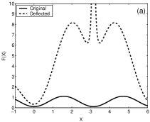
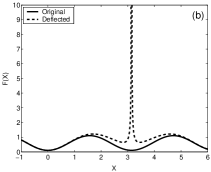
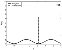
Figure 1: The effect of the deflection procedure on the function $f(x)=\sin^{2}(x)+0.1$, at the point $x^{*}=\pi$, for $\lambda=0.1$ (a), $\lambda=1$ (b), and $\lambda=10$ (c).

When the initial conditions of a $p$–periodic orbit are determined, the rest $(p-1)$ intersections of the orbit with the PSS (which can also be considered as initial conditions for the same orbit) are obtained through $(p-1)$ subsequent iterations of $\Phi(X)$ of Eq. (6). We determine the stability of the periodic orbit using established techniques (see for example Broucke, 1969; Hadjidemetriou, 1975; Pfenniger, 1984; Contopoulos & Magnenat, 1985; Skokos, 2001). The periodic orbit can either be stable (S) or unstable. We note that in 3D Hamiltonian systems we can have three different types of instability, namely simple unstable (U), double unstable (DU) and complex unstable ($\Delta$). The repetitive use of the deflection technique allows us to find several periodic orbits of a certain period, $p$. The proposed algorithm for the detection of periodic orbits is described in pseudocode in Table 1 (Parsopoulos & Vrahatis, 2004).

Table 1: The proposed algorithm. Note that $K$ denotes the maximum number of the periodic orbits that can be obtained in one run of the algorithm.

Input:	Hamiltonian $H$, period $p$, maximum number of deflections $K$.
Step 1	Set the stopping flag, $\textsl{SF}\leftarrow 0$, and the counter, $k\leftarrow 0$.
Step 2	While $(\textsl{SF}=0)$ Do
	Apply PSO
Step 3	If (PSO detected a periodic orbit, $X_{1}$) Then
	Compute all points $X_{2},\ldots,X_{p}$, of the periodic orbit,
	by iterating function $\Phi$ (Eq. (6)) on $X_{1}$.
Step 4	If $(k<K)$ Then
	Apply Deflection on $X_{1},\ldots,X_{p}$, and set
	the counter $k\leftarrow k+1$.
	Else
	Set $\textsl{SF}\leftarrow 1$
	End If
	Else
	Write “No further periodic orbit was detected”
	Set $\textsl{SF}\leftarrow 1$
	End If
	End While
Step 5	Report all detected periodic orbits.

4 Numerical results

Applying the scheme described in Sec. 3, we were able to find, apart from the known 1–periodic orbits of Hamiltonian (5) (Skokos et al., 2002a; Patsis et al., 2003b), many new 2D and 3D orbits of period 1. We also followed these orbits as the energy change, registering simultaneously their stability transitions and locating their bifurcations.

To investigate the performance of the algorithm, we searched for periodic orbits of multiplicity 1, at the region between the radial 4:1 and corotation resonances. In order to locate these orbits we used as search space, $S$, a subspace of the PSS, where the values of the initial conditions vary in some suitable intervals. Instead of letting all four variables, $x$, $z$, $\dot{x}$, $\dot{z}$, to vary simultaneously, which means that the search space will be 4–dimensional, we adopted a more efficient scheme, described below.

First we located the planar (2D) orbits of the system on the equatorial plain that exist in the 4-dimensional search space $S$. This was done in two phases. In the first phase, we located the 2D orbits starting perpendicular to the $y=0$ axis, having initial conditions of the form $(x,0,0,0)$. This means that the actual search space in this phase was 1–dimensional, as only the $x$ variable of the initial condition changed. Confining our search in an 1–dimensional search space, also allowed us to decrease the size $N$ of the swarm to $N=5$, using a smaller radius, $r=1$, of the neighborhood of every particle. All periodic orbits traced in this phase were registered and the corresponding initial conditions were transformed into maximizers of the objective function $f(X)$ through the deflection technique. The search for 2D periodic orbits was completed in a second phase by considering orbits starting not perpendicular to the $x$ axis, having initial conditions of the form $(x,0,\dot{x},0)$. In this stage the actual search space was 2–dimensional, while the swarm consisted of $N=10$ particles and the neighborhood radius was set to $r=2$. As the periodic orbits with $\dot{x}=0$ had already been found and prevented from been retraced in the previous stage of the application of PSO, we located planar orbits with $\dot{x}\neq 0$. Again, these periodic orbits were registered and prevented from been detected again, through deflection.

After the detection of the 2D periodic orbits of the system on the equatorial plane, we searched for purely 3D periodic orbits. Again the search was performed in different phases, keeping the dimensionality of the search space as low as possible. Since many 3D periodic orbits found by Skokos et al. (2002a) have initial conditions of the form $(x,z,0,0)$ and $(x,0,0,\dot{z})$, we first concentrated our tries to detect periodic orbits of this form. For such orbits, the actual search space of the PSO method is 2–dimensional, since two of the four variables are set equal to zero, so we used again $N=10$ and $r=2$. We note that orbits with $z=0$ and $\dot{z}=0$ had already been found and, thus, in these phases we detected actual 3D orbits. Instead of continuing our search by letting only one variable be equal to zero and having all the possible 3–dimensional search spaces, we preferred to search for orbits with initial conditions of the form $(x,z,\dot{x},\dot{z})$, because the physically most important periodic orbits had already been found. Therefore, the complete search for orbits with initial conditions of the form $(x,z,\dot{x},\dot{z})$ was actually performed, using $N=20$ and $r=3$.

The scheme of applying PSO in several phases is more efficient than the immediate search for orbits with initial conditions of the form $(x,z,\dot{x},\dot{z})$, because in every phase we were confined in search spaces of dimensionality lower than 4, which is a computationally easier task. Additionally, we traced the periodic orbits in a physically meaningful way for the particular system, as we found first the planar 2D orbits and then the spatial 3D orbits.

The main periodic orbits that we detected by using the PSO method are presented in the so–called ‘characteristic’ diagram (for definition see Contopoulos, 2002, Section 2.4.3) shown in Fig. 2.

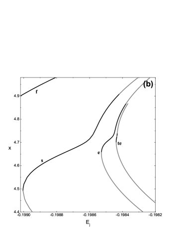
Figure 2: (a) Characteristic diagram of families x1, f, s, e, te. The dash-dotted curve is the section of the zero velocity surface with the $(E_{j},x)$ plane. In (b) we give the enlargement of the region included in the small rectangular in the upper right side of (a).

The diagram gives the $x$ coordinate of the initial condition of periodic orbits as a function of the energy $E_{j}$. Since we present in Fig. 2 only planar periodic orbits (i.e., $z=\dot{z}=0$), starting perpendicular to the $x$ axis (i.e., $\dot{x}=0$) with $y=0$ and $\dot{y}>0$, every point defines completely the initial condition of the orbit. Orbits on the $(x,y)$ plane with $\dot{x}\neq 0$ and orbits not lying on the $(x,y)$ plane are not represented on the characteristic diagram of Fig. 2. We also note that black curves correspond to stable periodic orbits, while gray curves indicate unstable periodic orbits without discriminating between their different instability types. In Fig. 2, we plot parts of the characteristic curves of the main 1–periodic family of the system, the so–called x1 family (Contopoulos & Papayannopoulos, 1980), and of the known (Patsis et al., 2003b) 2D f and s families, as well as the curves of two new families that were found using the PSO method. The characteristic curves of these two families are very close to each other and to the characteristic curve of family s. So, in order to clearly see them we enlarge in Fig. 2(b) the region enclosed in the small rectangular of Fig. 2(a). Also, we can see in Fig. 2(b) how close to each other are the various families of periodic orbits in this region of the characteristic diagram. This is the main difficulty that hinders other classical methods based on Newtonian techniques from locating periodic orbits in this region.

The two new families obtained through the proposed approach, exist for energies greater than a minimum energy value, similarly to families f and s. Since close to these minimum energy values the morphology of these families is influenced by the 8:1 and 10:1 resonances, we named these families as e and te families, respectively.

The e family exists for $E_{j}>-0.19853$. In Fig. 2(b), we see that the characteristic curve of the e family has two branches with stable orbits existing at the upper branch. In Fig. 3, we plot orbits of the e family for increasing values of the energy belonging to the upper branch (orbits (a), (b) and (c)), as well as to the lower branch (orbits (d) and (e)) of the characteristic.

Figure 3: Orbits of the 2D e family. From (a) to (b) and then to (c) we see the evolution of the orbital morphology along the upper branch of the characteristic of the e family as energy increases, while from (d) to (e) we see the evolution along the lower branch of the characteristic plotted in Fig. 2. Orbits (a) and (b) are stable while orbits (c), (d) and (e) are simple unstable. We remind that the bar major axis lies along the $y$ axis and the units are in Kpc.

Along the upper branch, we observe a smooth transition from a basically 8:1 morphology (orbit (a)) to a 10:1 morphology (orbit (c)) through an oval–shaped configuration (orbit (b)). We note that, as the energy increases, the orbits develop ‘corners’ along the minor axis of the bar ($x$ axis). An analogous transition from a 6:1 to an 8:1 morphology appears at the upper branch of the characteristic of the s family, as can be seen by comparing Figs. 3(a), (b) and (c) with Figs. 6(a), (b) and (c) of Patsis et al. (2003b). On the other hand, the morphology of the e family at the lower branch of its characteristic is always influenced by the 8:1 resonance (orbits (d) and (e)), and, as energy increases, the orbits develop loops (orbit (e)). We also note that the unstable orbits of the lower branch of the characteristic have almost straight segments parallel to the bar major axis ($y$ axis). Similar morphological evolution was observed also for the s family as can be seen by comparing Figs. 3(d) and (e) with Figs. 6(e) and (f) of Patsis et al. (2003b).

A new 2D family is born by bifurcation from the e family at $E_{j}\approx-0.19847$. We call it er1 following the nomenclature in Skokos et al. (2002a). The er1 family has a 9:1 morphology (Fig. 4), in analogy to the sr1 family (Fig. 6(d) of Patsis et al. (2003b)), which bifurcates from the s family and it is influenced by the 7:1 resonance.

Figure 4: Orbits of the 2D family er1. From (a) to (b) and then to (c) we see the orbital evolution of the family as the energy increases, moving away from its bifurcation point from family e. Orbits (a) and (b) are stable, while orbit (c) is simple unstable.

In Fig. 5, we see the morphological evolution of the ev1 3D family, which bifurcates from the e family at $E_{j}\approx-0.19849$.

Figure 5: 3D stable orbits of the ev1 family. For every orbit we plot its projection on the $(x,y)$, $(x,z)$ and $(y,z)$ planes. From (a) to (b) and then to (c) the energy increases moving away from the bifurcation point of ev1 from the e family.

We note that the projections of the ev1 orbits on the $(x,y)$ plane are similar to the planar 2D orbits of the e family for the same energies. So the ev1 orbits appear as oval-shaped and evolve to a 10:1 morphology.

The te family exists for $E_{j}>-0.198438$, and it has similar evolution to the e family. At the upper branch of its characteristic curve, there exist stable representatives of the family (orbits (a) and (b) of Fig. 6), while, at the lower branch, all orbits are unstable (orbits (d) and (e) of Fig. 6).

Figure 6: Orbits of the 2D te family. From (a) to (b) and then to (c) we see the evolution of the orbital morphology along the upper branch of the characteristic of the te family as energy increases, while from (d) to (e) we see the evolution along the lower branch of the characteristic depicted in Fig. 2. Orbits (a) and (b) are stable, orbits (c) and (e) are double unstable and orbit (d) is simple unstable.

Family te has a 10:1 morphology (Fig. 6(a)), which evolves to a morphology influenced by the 12:1 resonance (Fig. 6(c)). The orbits belonging to the upper branch of the characteristic curve develop ‘corners’ along the $x$ axis (Fig. 6(c)), while the orbits of the lower branch have segments parallel to the $y$ axis (Figs. 6(d) and (e)). The 2D family ter1 that bifurcates from family te at $E_{j}\approx-0.198434$ is influenced by the 11:1 resonance (Fig. 7),

Figure 7: Orbits of the 2D family ter1. From (a) to (b) and then to (c) we see the orbital evolution of the family as the energy increases, moving away from its bifurcation point from family te. Orbit (a) is stable, while orbits (b) and (c) are simple unstable.

while the 3D family tev1, which bifurcates from family te at $E_{j}\approx-0.198435$, has an oval–shaped projection on the $(x,y)$ plane (Fig. 8).

Figure 8: A 3D stable orbit of the tev1 family.

5 Discussion and conclusions

In this paper, we proposed and applied an algorithm for locating periodic orbits in a 3D galactic potential. Our numerical scheme is based on the transformation of a root–finding problem, i. e., solving Eq. (19), into a problem of detecting the global minimizers of function $f$ (Eq. 20). The detection of the minimizers is performed by the PSO method. This transformation also enables us to use a deflection technique, so that many periodic orbits are traced in one run of the algorithm. By using the proposed algorithm we were able to trace 2D and 3D periodic orbits close to the corotation region in the barred galaxy model described in Sec. 2. Our numerical results justify the usefulness of the new scheme, as well as its advantages, which springs from its ability to locate periodic orbits in regions where many periodic orbits coexist very close to each other, even when many of them are unstable. In addition, even if a periodic orbit is found, Newton–like methods cannot guarantee that repeating the search with a different initial guess will result in a new periodic orbit. The proposed scheme alleviates this problem.

In order to demonstrate the effectiveness of the proposed scheme, we discuss now in detail its application on the simplest case that we faced in the present paper. This case was the location of planar, 2D, orbits of period $p=1$, starting perpendicular to the $y=0$ axis, having initial conditions of the form $(x,0,0,0)$. Restricting the search for periodic orbits close to the corotation we set $E_{j}=0.1984$ and let $x$ varying in the region $3.5\leqslant x\leqslant 5.5$. In this case the search space of the PSO method was 1–dimensional and so we used a swarm of $N=5$ particles, while the neighborhood of every particle had radius $r=1$. Every iteration of the PSO method performed the evaluation of the objective function $f(X)$ (Eq. 20) with $p=1$, for $N=5$ times. This means that we computed the first intersection with the PSS of $N=5$ orbits or, in other words, we performed $N=5$ evaluations of $\Phi(X)$ (Eq. 6), which is the most time consuming computation in every iteration of the PSO method. In the particular application we asked the tracing of up to 15 periodic orbits in one run of the algorithm and we succeeded in locating all the planar 2D orbits of families e, te, er1 and ter1 existing in the search space, as well as, several banana–like orbits (not discussed in the paper) and orbits belonging to the s family. All the periodic orbits were located with accuracy of at least $10^{-10}$. The whole run performed about 1350 iterations of the PSO method (which means about 90 iterations per periodic orbit), involving a total of about 6750 evaluations of $\Phi(X)$. A main advantage of our approach is that it does not need good initial guesses close to the real initial conditions of the periodic orbits it traces. As an example we refer to the periodic orbit belonging to the ter1 family that was found by the above mentioned run. This orbit is simple unstable and the usual Newton iterative method for finding it, converges to its initial condition $x_{0}$ for initial guesses of $x$ satisfying $|x-x_{0}|\lesssim 7\cdot 10^{-5}$, after about 10 successive iterations. We note that in the general case of a 4–dimensional PSS every iteration of the Newton scheme involves the computation of the Jacobian matrix of the corresponding set of equations, which requires 4 evaluations of $\Phi(X)$ (see for example Pfenniger & Friedli, 1993). Thus, in principle, in order to be able to locate all the 2D periodic orbits in the interval $x\in[3.5,5.5]$ found by the PSO method, one should compute all the orbits with initial conditions on a grid of this interval whose grid step should at least be equal to $7\cdot 10^{-5}$. These procedure requires about 28500 evaluations of $\Phi(X)$, not taking into account the successive iterations of the Newton method to converge to the actual initial condition with the desired accuracy. We note that in the case of the ter1 periodic orbit this convergence requires about 10 evaluations of $\Phi(X)$. So it is evident that the computational effort needed by our numerical scheme is significantly lower with respect to the Newton iterative method even in the simple case of the 1–dimensional search space.

As we pointed out, the main problem that Newton–like techniques face in cases where many periodic orbits coexist very close to each other, is that they need a very good initial guess of the position of the periodic orbit in order to find it. This difficulty of the Newton iterative schemes is well known and some efforts to improve their efficiency have already been done. As an example, we refer to the paper of Pfenniger & Friedli (1993) where the authors evaluate the initial conditions in every successive iteration of the Newton scheme by an appropriate least squares technique. We emphasize that our approach is completely different as we do not try to find the roots of the system of Eq. (19) but we transform this problem into a minimization one. We also note that our scheme uses only the values of function $\Phi$ (Eq.  6) and not its derivatives like Newton iterative techniques do. This makes our computation easier and more accurate, since the usual method to evaluate the derivatives of function $\Phi$, which is not known in a close analytical form, is to approximate them by finite differences.

Summarizing the main advantages of the proposed algorithm with respect to Newton–like methods we could mention that our method is faster, it is simple and can be implemented easily, it works using function values solely, and also it has the ability to locate many periodic orbits per run.

The orbital behavior of the e and te families and their bifurcations, which were detected by the proposed scheme, as well as the behavior of the s family (Patsis et al., 2003b), helps us to establish the general behavior of the families existing beyond the radial 4:1 resonance gap in our model. The morphology of the basic 2D families are influenced by two successive even resonances: the s family is influenced by the 6:1 and 8:1 resonances, the e family is influenced by the 8:1 and 10:1 resonances and the te family by the 10:1 and 12:1 resonances. From these families, 2D families influenced by the in-between odd resonances bifurcate: sr1 is influenced by the 7:1 resonance, er1 by the 9:1 resonance and ter1 by the 11:1 resonance. In addition, the main 3D bifurcations of the s, e and te families (sv1, ev1, tev1 families respectively) have, in general, projections on the $(x,y)$ plane similar to the main families. This is in accordance with the observed frequency of the various inner rings morphology (Buta, 1995), as proposed by Patsis et al. (2003b).

References

- Athanassoula (1984) Athanassoula E., 1984, Phys. Rep., 114, 319
- Bonabeau et al. (1999) Bonabeau E., Dorigo M., Theraulaz G., 1999, Swarm Intelligence: From Natural to Artificial Systems, New York, Oxford University Press
- Broucke (1969) Broucke R., 1969, NASA Techn. Rep., 32, 1360
- Buta (1995) Buta R., 1995, ApJS, 96, 39
- Clerc & Kennedy (2002) Clerc M., Kennedy J., 2002, IEEE Trans. Evol. Comput., 6(1), 58
- Contopoulos (1980) Contopoulos G., 1980, A&A, 81, 198
- Contopoulos (2002) Contopoulos G., 2002, Order and Chaos in Dynamical Asronomy, Berlin, Springer Verlag
- Contopoulos & Grosbøl (1989) Contopoulos G., Grosbøl P., 1989, A&AR 1, 261
- Contopoulos & Magnenat (1985) Contopoulos G., Magnenat P., 1985, Celest. Mech., 37, 387
- Contopoulos & Papayannopoulos (1980) Contopoulos G., Papayannopoulos Th., 1980, A&A, 92, 33
- Eberhart & Kennedy (1995) Eberhart R.C., Kennedy J., 1995, Proc. Sixth Symp. Micro Mach. Hum. Sci., 39
- Fogel (2000) Fogel D.B., 2000, IEEE Spectrum, 37(2), 26
- Hadjidemetriou (1975) Hadjidemetriou J., 1975, Celest. Mech., 12, 255
- Kennedy & Eberhart (2001) Kennedy J., Eberhart R.C., 2001, Swarm Intelligence, San Francisco, Morgan Kaufmann
- Lieberman & Lichtenberg (1992) Lieberman M.A., Lichtenberg A.J., 1992, Regular and Chaotic Dynamics, Springer Verlag
- Magoulas et al. (1997) Magoulas G.D., Plagianakos V.P., Vrahatis M.N., 1997, Nonlinear Analysis Theory Methods & Applications, 30(7), 4545
- Millonas (1994) Millonas M.M., 1994, Artificial Life III, 417
- Miyamoto & Nagai (1975) Miyamoto M., Nagai R., 1975, PASJ, 27, 533
- Parsopoulos & Vrahatis (2002) Parsopoulos K.E., Vrahatis M.N., 2002, Natural Computing, 1 (2-3), 235
- Parsopoulos & Vrahatis (2004) Parsopoulos K.E., Vrahatis M.N., 2004, IEEE Transactions on Evolutionary Computation, 8 (3), 211
- Patsis (2004) Patsis P.A., 2004, MNRAS, (submitted)
- Patsis et al. (2002) Patsis P.A., Skokos Ch., Athanassoula E., 2002, MNRAS, 337, 578
- Patsis et al. (2003a) Patsis P.A., Skokos Ch., Athanassoula E., 2003a, MNRAS, 342, 69
- Patsis et al. (2003b) Patsis P.A., Skokos Ch., Athanassoula E., 2003b, MNRAS, 346, 1031
- Pfenniger (1984) Pfenniger D., 1984, A&A, 134, 373
- Pfenniger (1996) Pfenniger D., 1996, in Buta R., Crocker D. A., Elmegreen B. G., eds, ASp Conf. Ser. Vol. 91, Barred galaxies, Astron. Soc. Pac., San Francisco, 273
- Pfenniger & Friedli (1993) Pfenniger D., Friedli D., 1993, A&A, 270, 561
- Schwefel (1994) Schwefel H.–P., 1994, Zurada J.M., Marks II R.J., Robinson C.J., eds, Computational Intelligence: Imitating Life
- Sellwood & Wilkinson (1993) Sellwood J., Wilkinson A., 1993, Rep. Prog. Phys., 56, 173
- Skokos (2001) Skokos Ch., 2001, Phys. D, 159, 155
- Skokos et al. (2002a) Skokos Ch., Patsis P.A., Athanassoula E., 2002a, MNRAS, 333, 847
- Skokos et al. (2002b) Skokos Ch., Patsis P.A., Athanassoula E., 2002b, MNRAS, 333, 861
- Storn & Price (1997) Storn R., Price K., 1997, J. Global Optimization, 11, 341
- Trelea (2003) Trelea I.C., 2003, Information Processing Letters, 85, 317