Exploring the relativistic regime with Newtonian hydrodynamics:
An improved effective gravitational potential for supernova simulations

We investigate the possibility approximating relativistic effects in hydrodynamical simulations of stellar core collapse and post-bounce evolution by using a modified gravitational potential in an otherwise standard Newtonian hydrodynamic code. Different modifications of a previously introduced effective relativistic potential are discussed. Corresponding hydrostatic solutions are compared with solutions of the TOV equations, and hydrodynamic simulations with two different codes are compared with fully relativistic results. One code is applied for one- and two-dimensional calculations with a simple equation of state, and employs either the modified effective relativistic potential in a Newtonian framework or solves the general relativistic field equations under the assumption of the conformal flatness condition (CFC) for the three-metric. The second code allows for full-scale supernova runs including a microphysical equation of state and neutrino transport based on the solution of the Boltzmann equation and its moments equations. We present prescriptions for the effective relativistic potential for self-gravitating fluids to be used in Newtonian codes, which produce excellent agreement with fully relativistic solutions in spherical symmetry, leading to significant improvements compared to previously published approximations. Moreover, they also approximate qualitatively well relativistic solutions for models with rotation.

1 Introduction

It is a well known fact that gravity plays an important role during all stages of a core collapse supernova. Gravity is the driving force that at the end of the life of massive stars overcomes the pressure forces and causes the collapse of the stellar core. Furthermore, the subsequent supernova explosion results from the fact that various processes tap the enormous amount of gravitational binding energy released during the formation of the proto-neutron star. General relativistic effects are important for this process and cannot be neglected in quantitative models because of the increasing compactness of the proto-neutron star. Therefore, it is important to include a proper treatment of general relativity or an appropriate approximation in the numerical codes that one uses to study core collapse supernovae.

Recently Liebendörfer et al. (2005) performed a comparison of the results obtained with the supernova simulation codes Vertex and Agile-BoltzTran which both solve the Boltzmann transport equation for neutrinos. The Vertex code (see Rampp & Janka 2002) is based on the Newtonian hydrodynamics code Prometheus (Fryxell et al. 1990) and utilizes a generalised potential to approximate relativistic gravity. The Agile-BoltzTran code of the Oak Ridge-Basel group (Liebendörfer et al. 2001, 2002, 2004, 2005) is a fully relativistic (1D) hydrodynamics code. The comparison showed that both codes produce qualitatively very similar results except for some small (but growing) quantitative differences occurring in the late post-bounce evolution. Inspired by this comparison we explored improvements of the effective relativistic potential used by Rampp & Janka (2002) in order to achieve an even better agreement than that reported by Liebendörfer et al. (2005). To this end we tested different variants of approximations to relativistic gravity employing two simulation codes.

On the one hand purely hydrodynamic simulations were performed with the code CoCoNuT of Dimmelmeier et al. (2002a, 2005) assuming spherical or axial symmetry. This code optionally either uses a Newtonian (or alternatively an effective relativistic) gravitational potential in a Newtonian treatment of the hydrodynamic equations or solves the general relativistic equations of fluid dynamics and the relativistic field equations. The latter are formulated under the assumption of the conformal flatness condition (CFC) for the three-metric, also known as the Isenberg–Wilson–Mathews approximation (Isenberg 1978; Wilson et al. 1996), which is identical to solving the exact general relativistic equations in spherical symmetry. This allows for a direct comparison of different effective relativistic potentials with a fully relativistic treatment in both spherically symmetric and axisymmetric simulations using the same code.

On the other hand, we used the computationally expensive Vertex code (Rampp & Janka 2002) for spherically symmetric supernova simulations including neutrino transport and a microphysical equation of state (EoS). The results of these calculations performed with different effective relativistic potentials are compared with those obtained with the general relativistic Agile-BoltzTran code of the Oak Ridge-Basel group (cf. Liebendörfer et al. 2005).

In this paper we discuss the results of our test calculations and present improved effective relativistic potentials which are simple to implement without modifying the Newtonian equations of hydrodynamics in an existing code, and which approximate the results of general relativistic simulations very well.

The paper is organised as follows: In Sect. 2 we describe the effective relativistic potentials used in this investigation. In Sect. 3 we briefly discuss the most important features of the numerical codes we used for our hydrodynamic simulations. In Sect. 4 we present the results obtained by applying the effective relativistic potentials in spherically symmetric simulations of supernova core collapse and to neutron star models, while Sect. 5 is devoted to a discussion of the multi-dimensional simulations of rotational supernova core collapse. Finally, in Sect. 6 we summarise our findings and draw some conclusions.

Throughout the article, we use geometrised units with $c=G=1$.

2 Effective relativistic potential

Approximating the effects of general relativistic gravity in a Newtonian hydrodynamics code may be attempted by using an effective relativistic gravitational potential $\Phi_{\mathrm{eff}}$ which mimics the deeper gravitational well of the relativistic case. In the following Sects. 2.1 and 2.2, several of these effective relativistic potentials will be discussed.

2.1 TOV potential for a self-gravitating fluid

For a self-gravitating fluid it is desirable that an effective relativistic potential reproduces the solution of hydrostatic equilibrium according to the Tolman–Oppenheimer–Volkoff (TOV) equation. With this requirement in mind and comparing the relativistic equation of motion (cf. van Riper 1979; Baron et al. 1989) with its Newtonian analogon, Rampp & Janka (2002) rearranged the relativistic terms into an effective relativistic potential (see Kippenhahn & Weigert 1990, for the hydrostatic, neutrino-less case).

Thus for spherically symmetric simulations using a Newtonian hydrodynamics code the idea is to replace the Newtonian gravitational potential

$$\Phi(r)=-4\pi\int_{0}^{\infty}\!\!\mathrm{d}r^{\prime}\,r^{\prime 2}\frac{\rho}{|r-r^{\prime}|}$$ (1)

by the TOV potential

$$\Phi_{\mathrm{TOV}}(r) = -4\pi\int_{r}^{\infty}\frac{\mathrm{d}r^{\prime}}{r^{\prime 2}}\left(\frac{m_{\mathrm{TOV}}}{4\pi}+r^{\prime 3}(P+{p}_{\nu})\right)$$ (2)

$$\qquad\qquad\times\frac{1}{\Gamma^{2}}\left(\frac{\rho+e+P}{\rho}\right),$$

to obtain the effective relativistic potential $\Phi_{\mathrm{eff}}$ as

$$\Phi_{\mathrm{eff}}=\Phi_{\mathrm{TOV}}.$$ (3)

Here $\rho$ is the rest-mass density, $e=\rho\epsilon$ is the internal energy density with $\epsilon$ being the specific internal energy, and $P$ is the gas pressure. The TOV mass is given by

$$m_{\mathrm{TOV}}(r)=4\pi\int_{0}^{r}\mathrm{d}r^{\prime}\,r^{\prime 2}\!\left(\rho+e+E+\frac{vF}{\Gamma}\right),$$ (4)

where $p_{\nu}$, $E$, and $F$ are the neutrino pressure, the neutrino energy density, and the neutrino flux, respectively (Baron et al. 1989; Rampp & Janka 2002).

The fluid velocity $v$ is identified with the local radial velocity calculated by the Newtonian code and the metric function $\Gamma$ is given by

$$\Gamma=\sqrt{1+v^{2}-\frac{2m_{\mathrm{TOV}}}{r}}.$$ (5)

The velocity-dependent terms were added for a closer match with the general relativistic form of the equation of motion (van Riper 1979; Baron et al. 1989). In the treatment of neutrino transport general relativistic redshift and time dilation effects are included, but for reasons of consistency with the Newtonian hydrodynamics part of the code the distinction between coordinate and proper radius is ignored in the relativistic transport equations (for details, see Sect. 3.7.2 of Rampp & Janka 2002). The quality of this approach was ascertained by a comparison with fully relativistic calculations (Rampp & Janka 2002; Liebendörfer et al. 2005).

In order to calculate the effective relativistic potential for multi-dimensional flows we substitute the “spherical contribution” $\overline{\!\Phi\!}\,(r)$ to the multi-dimensional Newtonian gravitational potential

$$\Phi(r,\theta,\varphi)=-\int_{V}\!\!\mathrm{d}r^{\prime}\,\mathrm{d}\theta^{\prime}\,\mathrm{d}\varphi^{\prime}\,r^{\prime 2}\sin\theta^{\prime}\frac{\rho}{|\mbox{\boldmath$r$}-\mbox{\boldmath$r^{\prime}$}|}$$ (6)

by the TOV potential $\overline{\!\Phi\!}\,_{\mathrm{TOV}}$:

$$\Phi_{\mathrm{eff}}=\Phi-\overline{\!\Phi\!}\,+\overline{\!\Phi\!}\,_{\mathrm{TOV}}.$$ (7)

Here $\overline{\!\Phi\!}\,(r)$ and $\overline{\!\Phi\!}\,_{\mathrm{TOV}}$ are calculated according to Eqs. (1) and (2), respectively, however with the hydrodynamic quantities $\rho$, $e$, $P$, $v$ and the neutrino quantities $E$, $F$, $p_{\nu}$ being replaced by their corresponding angularly averaged values. Note that $v$ here refers to the radial component of the velocity, only.

2.2 Modifications of the TOV potential

In a recent comparison Liebendörfer et al. (2005) found that gravity as described by the TOV potential in Eq. (3) overrates the relativistic effects, because in combination with Newtonian kinematics it tends to overestimate the infall velocities and to underestimate the flow inertia in the pre-shock region. Thus, supposedly via the nonlinear dependence of $\Phi_{\mathrm{eff}}$ on $e$ and $P$ the compactness of the proto-neutron star is overestimated, with this tendency increasing at later times after core bounce. Consequently, the neutrino luminosities and the mean energies of the emitted neutrinos are larger than in the corresponding relativistic simulation.

In order to reduce these discrepancies – without sacrificing the simplicity of Newtonian dynamics – we tested several modifications of the TOV potential, Eqs. (2), which all act to weaken it. In particular, we studied the following variations:

Case A:

In the integrand of Eq. (4) a factor $\Gamma$, Eq. (5) is added. Since $\Gamma<1$ this reduces the gravitational TOV mass used in the potential.

Case B:

In Eq. (4) the internal gas energy density and the neutrino terms are set to zero, $e=E=F=0$, which again decreases the gravitational TOV mass.

Case C:

In Eq. (2) the internal gas energy is set to zero, $e=0$, which directly weakens the TOV potential.

Case D:

In the equation for the TOV potential, Eq. (2), $m_{\mathrm{TOV}}$ is replaced by $\frac{1}{2}(m_{\mathrm{TOV}}+m_{\mathrm{g}})$. Here a Newtonian gravitational mass is defined as $m_{\mathrm{g}}=m_{\mathrm{r}}-m_{\mathrm{b}}$ with the rest mass $m_{\mathrm{r}}=4\pi\int_{0}^{r}\mathrm{d}r^{\prime}\,r^{\prime 2}\rho$ and the mass equivalent of the binding energy $m_{\mathrm{b}}=2\pi|\int_{0}^{r}\mathrm{d}r^{\prime}\,r^{\prime 2}\rho\,\Phi|$. As $m_{\mathrm{g}}<m_{\mathrm{TOV}}$, the strength of the potential is reduced.

Case E:

Both in the equation for the TOV potential, Eq. (2), and the equation for the TOV mass, Eq. (4), we set $e=0$.

Case F:

In the equation for the TOV potential, Eq. (2), we set $\Gamma=1$. As $\Gamma<1$ otherwise, this weakens the potential.

Case G:

In the expression for $\Gamma$, Eq. (5), the velocity is set to zero, $v=0$. Hence, $\Gamma^{-2}$ increases in Eq. (2). This modification is used to also test a potential which is even stronger than the unmodified TOV potential.

In addition to these cases with a modified version of the TOV potential, we use the following notations:

Case N:

This denotes the purely Newtonian runs with “regular” Newtonian potential.

Case R:

This is the “reference” case with the TOV potential as defined by Eq. (2).

Case GR:

This case refers to fully relativistic simulations with either the code CoCoNuT or the Agile-BoltzTran neutrino radiation-hydrodynamics code of the Oak Ridge-Basel collaboration.

Note that setting the internal energy density $e$ to zero in Case B is unambiguous when a simple EoS is used and the particle rest masses are conserved. In general, however, particles can be created and destroyed, or bound states can be formed (e.g., in pair annihilation processes or nuclear reactions, respectively). Then only the sum of the rest mass energy and internal energy per nucleon – both appear in Eqs. (2, 4) only combined in form of the “relativistic energy” per unit of mass, $(\rho+e)/\rho$ – is well defined, but not the individual parts. Therefore there exists ambiguity with respect to which contribution to the energy is set to zero. In order to assess a possible sensitivity of the core collapse results to this ambiguity, we tried two different variants of Case B in our Vertex simulations with microphysical EoS. On the one hand we used $\widetilde{e}=E=F=0$ in Eq. (4), with $\widetilde{e}$ being the internal energy density plus an energy normalization given by the EoS of Lattimer & Swesty (1991), $\widetilde{e}=(\rho+e)-\rho\,(m_{\mathrm{n}}-\Delta)/m_{\mathrm{u}}$ (where $m_{\mathrm{u}}=1.66\times 10^{-24}\mathrm{\ g}$ is the atomic mass unit, $m_{\mathrm{n}}$ the neutron rest mass, and $\Delta=8.8\mathrm{MeV}$). On the other hand we tested $e^{\ast}=E=F=0$ with $e^{\ast}$ being $\widetilde{e}$ without this energy normalization, i.e. $e^{\ast}=(\rho+e)-\rho\,m_{\mathrm{n}}/m_{\mathrm{u}}$. Nucleons are then assumed to contribute to the TOV mass, Eq. (4), with the vacuum rest mass of the neutron, increasing the mass integral and reducing $\Gamma$ (Eq. (5) relative to the first case, thus making the effective relativistic potential a bit stronger again. In order to compensate for this we also set $p_{\nu}=0$ in the TOV potential, Eq. (2). Both variants are found to yield extremely similar results and we therefore will discuss only one of them (the first variant) as Case B for the Vertex simulations.

Ideally, a Newtonian simulation with an effective relativistic potential not only yields a solution of the TOV structure equations for an equilibrium state (as does Case R), but in addition closely reproduces the results from a relativistic simulation (Case GR) during a dynamic evolution. Applying the modifications of the TOV potential listed above, we find that Cases A to D yield improved results as compared to Case R, while Cases E to G either weaken the potential too much or are very close to Case R. These findings are detailed in Sect. 4 and 5.

2.3 Theoretical motivation

There are (at least) two basic requirements which appear desirable for an effective relativistic potential in a Newtonian simulation. Firstly, the far field limit of the fully relativistic treatment should be approximated reasonably well in order to follow the long-term accretion of the neutron star and the associated growth of its baryonic mass. Secondly, the hydrostatic structure of the neutron star should well fit the solution of the TOV equations.

The second point will be discussed in detail in Sect. 4.1. A closer consideration of the first point suggests the modified effective relativistic potential of Case A as promising, and in fact it turns out to be the most preferable choice concerning consistency and quality of the results. The other cases listed in Sect. 2.2 are mostly ad hoc modifications of the original effective relativistic potential of Eqs. (2)–(4) (Case R) with the aim to reduce its strength, which was found to overestimate the effects of gravity compared to fully relativistic simulations in previous work (Liebendörfer et al. 2005). These cases are also discussed here for reasons of comparison and completeness.

In Eq. (4) the hydrodynamic quantities (like rest-mass density $\rho$ plus extra terms) are integrated over volume. In the Newtonian treatment there is no distinction between coordinate volume and local proper volume. Performing the integral of Eq. (4) therefore leads to a mass – used as the mass which produces the gravitational potential in Eqs. (2) and (3) – which is larger than the baryonic mass, $m_{\mathrm{b}}=4\pi\int\mathrm{d}r^{\prime}\,r^{\prime 2}\rho$. In particular, it is also larger than the gravitational mass in a consistent relativistic treatment, which is the volume integral of the total energy density and includes the negative gravitational potential energy of the compact object. The latter reduces the gravitational mass relative to the baryonic mass by the gravitational binding energy of the star (see, e.g., Shapiro & Teukolsky 1983, page 125 for a corresponding discussion). Therefore, the effective relativistic potential introduced by Rampp & Janka (2002) [our Case R, Eqs. (2–4)] cannot properly reproduce the far field limit of the relativistic case and thus overestimates the effects of gravity. This particularly applies to the infall velocities of the stellar gas ahead of the supernova shock, as shown in Liebendörfer et al. (2005).

Introducing an extra factor $\Gamma$ in the integral of Eq. (4) for the TOV mass is motivated by the following considerations (where for reasons of simplicity contributions from neutrinos, though important, are neglected and spherical symmetry is assumed): In the relativistic treatment the total (gravitating) mass of the star is given as

$$m_{\mathrm{g}}=4\pi\int_{0}^{\infty}\!\!\mathrm{d}r^{\prime}\,r^{\prime 2}(\rho+e),$$ (8)

where $\mathrm{d}V^{\prime}=4\pi\mathrm{d}r^{\prime}\,r^{\prime 2}$ is the coordinate volume element, whereas the baryonic mass is

$$m_{\mathrm{b}}=4\pi\int_{0}^{\infty}\!\!\mathrm{d}r^{\prime}\,r^{\prime 2}\Gamma^{-1}\rho,$$ (9)

with $\mathrm{d}{\cal V}^{\prime}=4\pi\mathrm{d}r^{\prime}r^{\prime 2}\Gamma^{-1}$ being the local proper volume element. The factor $\Gamma^{-1}>1$ in the integrand of $m_{\mathrm{b}}$ thus ensures that $m_{\mathrm{b}}>m_{\mathrm{g}}$. The integral for $m_{\mathrm{g}}$ can also be written as

$$m_{\mathrm{g}}=4\pi\int_{0}^{\infty}\!\!\mathrm{d}r^{\prime}\,r^{\prime 2}\,\frac{\Gamma}{\Gamma}\,(\rho+e)=\int_{0}^{\infty}\!\!\mathrm{d}{\cal V}^{\prime}\,\Gamma\,(\rho+e).$$ (10)

Since in Newtonian hydrodynamics no distinction is made between coordinate and proper volumes, one may identify $\mathrm{d}{\cal V}^{\prime}\equiv\mathrm{d}V^{\prime}$, consistent with the rest of our Newtonian code. This leaves the additional factor $\Gamma$ in the integrand of Eq. (10), leading to a redefined TOV mass used for computing the effective relativistic potential in Case A,

$$\widetilde{m}_{\mathrm{TOV}}(r)=4\pi\int_{0}^{r}\mathrm{d}r^{\prime}\,r^{\prime 2}\Gamma\left(\rho+e+E+\frac{vF}{\Gamma}\right).$$ (11)

The fact that a factor $\Gamma^{-1}$ in the volume integral establishes the relation between gravitating mass, Eq. (8), and baryonic mass, Eq. (9), in the relativistic case suggests that the factor $\Gamma<1$ in Eq. (11) might lead to a suitable reduction of the overestimated effective potential that results when the original TOV mass of Eq. (4) is used in Eqs. (2) and (5). Indeed, a comparison of the integral of Eq. (11) for large $r$ with the rest-mass energy of a neutron star reduced by its binding energy at time $t$ (computed from the emitted neutrino energy, $\int_{0}^{t}\mathrm{d}t^{\prime}\,L_{\nu}(t^{\prime})$ with $L_{\nu}$ being the neutrino luminosity) reveals very good agreement.

The arguments given above only provide a heuristic justification for the manipulation of the TOV potential proposed in Case A. A deeper theoretical understanding and more rigorous analytical analysis of its consequences and implications is certainly desirable, but beyond the scope of the present paper. We plan to return to this question in future work.

3 Numerical methods

In the following we briefly introduce the two numerical codes used for the simulations presented in this work. The codes are based on state-of-the-art numerical methods for hydrodynamics and neutrino transport coupled to gravity, and were used to simulate stellar core collapse and supernova explosions.

3.1 Hydrodynamic code without transport

The purely hydrodynamic simulations are performed with the code CoCoNuT developed by Dimmelmeier et al. (2002a, b) with a metric solver based on spectral methods as described in Dimmelmeier et al. (2005). The code optionally uses either a Newtonian gravitational potential (or an effective relativistic potential, see Sect. 2), or the general relativistic field equations for a curved spacetime in the ADM 3 + 1-split under the assumption of the conformal flatness condition (CFC) for the three-metric. The (Newtonian or general relativistic) hydrodynamic equations are consistently formulated in conservation form, and are solved by high-resolution shock-capturing schemes based upon state-of-the-art Riemann solvers and third-order cell-reconstruction procedures. Neutrino transport is not included in the code. A simple hybrid ideal gas EoS is used that consists of a polytropic contribution describing the degenerate electron pressure and (at supranuclear densities) the pressure due to repulsive nuclear forces, and a thermal contribution which accounts for the heating of the matter by shocks:

$$P=P_{\mathrm{p}}+P_{\mathrm{th}},$$ (12)

where

$$P_{\mathrm{p}}=K\rho^{\gamma},\qquad P_{\mathrm{th}}=\rho\epsilon_{\mathrm{th}}(\gamma_{\mathrm{th}}-1),$$ (13)

and $\epsilon_{\mathrm{th}}=\epsilon-\epsilon_{\mathrm{p}}$. The polytropic specific internal energy $\epsilon_{\mathrm{p}}$ is determined from $P_{\mathrm{p}}$ by the ideal gas relation in combination with continuity conditions in the case of a discontinuous $\gamma$. In that case, the polytropic constant $K$ also has to be adjusted (for more details, see Dimmelmeier et al. 2002a; Janka et al. 1993).

The CoCoNuT code utilizes Eulerian spherical coordinates $\{r,\theta,\varphi\}$, and thus axially or spherically symmetric configurations can be easily simulated. For the core collapse simulations discussed in Sects. 4.1 and 5, the finite difference grid consists of 200 logarithmically spaced radial grid points with a central resolution of $500\mathrm{\ m}$. A small part of the grid covers an artificial low-density atmosphere extending beyond the core’s outer boundary. The spectral grid of the metric solver is split into 6 radial domains with 33 collocation points each. In order to be able to accurately follow the dynamics, the domain boundaries adaptively contract towards the centre during the collapse, as described in Dimmelmeier et al. (2005). For the migration test (Sect. 4.3) the finite difference grid consists of 250 logarithmically spaced radial grid points, of which 60 and 190 cover the neutron star and the atmosphere, respectively. For the two-dimensional simulations of rotational core collapse (Sect. 5) the finite difference and spectral grids are extended by 30 and 17 equidistant angular grid points, respectively.

Even when using spectral methods the calculation of the spacetime metric is computationally expensive. Hence, in the relativistic spherical (rotational) core collapse simulations the metric is updated only once every 10/1/50 (100/10/50) hydrodynamic time steps before/during/after core bounce, and extrapolated in between. In the migration test the update is performed every 10th step during the entire evolution. The numerical adequacy of this procedure is tested and discussed in detail in Dimmelmeier et al. (2002a).

The quality of the CFC approximation has been tested comprehensively in the context of supernova core collapse and for neutron star models (Cook et al. 1996; Dimmelmeier et al. 2002a; Shibata & Sekiguchi 2004; Dimmelmeier et al. 2005; Cerdá-Durán et al. 2004). For single stellar configurations the CFC approximation is very accurate as long as neither the compactness of the star is extremely relativistic nor its rotation is too fast and differential. Both criteria are well fulfilled during supernova core collapse. Concerning core collapse simulations of rapidly and strongly differentially rotating configurations at very high densities, we recently found that the CFC approximation yields excellent agreement with formulations solving the exact spacetime metric even in this extreme regime (Ott et al. 2005).

As the three-metric of any spherically symmetric spacetime can be written in a conformally flat way, the spherical CFC simulations presented in Sect. 4.1 and 4.3 involve no approximation, i.e., the exact Einstein equations are solved in these cases.

3.2 Hydrodynamic code with neutrino transport

The Vertex neutrino-hydrodynamics code solves the conservation equations of Newtonian hydrodynamics in their Eulerian and conservative form using the PPM-based Prometheus code (Fryxell et al. 1990). The neutrino transport is treated by determining iteratively a solution of the coupled set of moments equations and Boltzmann equation, achieving closure by a variable Eddington factor method (Rampp & Janka 2002). See the latter reference also for details about the coupling between the hydrodynamics and neutrino transport parts of the Vertex code. The models presented in this paper are computed with the equation of state of Lattimer & Swesty (1991), in agreement with the choice of input physics in the work of Liebendörfer et al. (2005), where results obtained with the Vertex code were compared with those from the Newtonian and fully relativistic calculations with the Agile-BoltzTran code of the Oak Ridge-Basel collaboration.

In order to compare the results presented here with those of the calculations of Liebendörfer et al. (2005) we used the same set of neutrino interaction rates as picked for Model G15 in Liebendörfer et al. (2005), and exactly the same parameters for the numerical setup (e.g., the grids for hydrodynamics and neutrino transport). Information about this setup can be found in Liebendörfer et al. (2005). The initial model for our calculations is the $15M_{\odot}$ progenitor model “s15s7b2” from Woosley & Weaver (1995).

Since solving the neutrino transport problem is computationally quite expensive we performed calculations only for Cases A, B, and F (as defined in Sect. 2.2) with the Vertex code. The quality of these results is then compared to the fully relativistic treatment of the Agile-BoltzTran code.

3.3 Hydrodynamics and implementation of the effective relativistic potential

The implementation of an effective relativistic gravitational potential or of an effective relativistic gravitational force as its derivative into existing Newtonian hydrodynamics codes is straightforward and does not differ from the use of the Newtonian potential or force.

The equations solved by the two codes used for our simulations are described in much detail in previous publications (see, e.g., Rampp & Janka 2002; Müller & Steinmetz 1995; Dimmelmeier et al. 2002a, 2005, and references therein). The implementation of the source terms of the gravitational potential as discussed in Müller & Steinmetz (1995) is also applied for the handling of the effective relativistic potentials investigated in this work. The only specific feature here is the mutual dependence of $\Gamma$ and $m_{\mathrm{TOV}}$, which is either accounted for by a rapidly converging iteration or by taking $\Gamma$ from the old time step in the update of $m_{\mathrm{TOV}}$, when the changes during the time steps are sufficiently small.

Since the actual form of the gravitational source term is unspecified in the conservation laws of fluid dynamics, the Newtonian potential can be replaced by the effective relativistic potentials investigated in the current work in a technically straightforward way. Solving an equation for the internal plus kinetic energy (as in our codes) requires a treatment of the gravity source term in this equation that is consistent with its implementation in the equation of momentum.

Of course, the effective potential must be investigated concerning its consequences for the conservation of momentum and energy. Since a potential constructed according to Eqs. (2, 4) does not satisfy the Poisson equation, the momentum equation cannot be cast into a conservation form (cf. Shu 1992, Part I, Chapter 4). As a consequence, the total linear momentum is strictly conserved only when certain assumptions about the symmetry of the matter distribution are made, for example in the case of spherical symmetry or axially symmetric configurations with equatorial symmetry, or when only one octant is modeled in the three-dimensional case. In axisymmetric simulations the conservation of specific angular momentum is fulfilled as well, when using the effective relativistic potential. In general, however, a sufficient quality of momentum (and angular momentum) conservation has to be verified by inspecting the numerical results.

The long-range nature of gravity prohibits to have an equation in pure conservation form for the total energy, i.e., for the sum of internal, kinetic, and gravitational energy (Shu 1992, Part I, Chapter 4). In contrast to the Newtonian case, however, our effective relativistic potential does also not allow one to derive a conservation equation for the total energy integrated over all space. Monitoring global energy conservation in a simulation with effective relativistic potential therefore requires integration of the gravitational source terms over all cells in time. If the local effects of relativistic gravity are convincingly approximated – as measured by good agreement with static solutions of the TOV equation and with fully relativistic, dynamical simulations – there is confidence that the integrated action of the employed gravitational source term approximates well also the global conversion between total kinetic, internal, and gravitational energies found in a relativistic simulation.

The recipes for approximating general relativity should be applicable equally well in hydrodynamic codes different from our (Eulerian) PPM schemes, provided the effects of gravity are consistently treated in the momentum and energy equations. The proposed effective potentials are intended to yield a good representation of the effects of relativistic gravity in particular in the context of stellar core collapse and neutron star formation. For our approximation to work well, the fluid flow should be subrelativistic. The numerical tests described in the following sections show that velocities up to about 20% of the speed of light are unproblematic.

4 Simulations in spherical symmetry

4.1 Supernova core collapse with simplified equation of state

We first test the quality of the TOV potential and its various modifications as an effective relativistic potential in the moderately relativistic regime by evolving models of supernova core collapse with the simple EoS described in Sect. 3.1. Using the CoCoNuT code we are able to perform a direct comparison with a Newtonian version of the code (employing either the Newtonian, TOV, or modified TOV potential) against the relativistic version in a curved spacetime.

The initial models are polytropes, which mimic an iron core supported by electron degeneracy pressure, with a central density $\rho_{\rm c\,i}=10^{10}{\rm\ g\ cm}^{-3}$ and EoS parameters $\gamma_{\mathrm{i}}=4/3$ and $K=4.897\times 10^{14}$ (in cgs units). To initiate the collapse, the initial adiabatic index is reduced to $\gamma_{1}<\gamma_{\mathrm{i}}$. At densities $\rho>\rho_{\rm nuc}\equiv 2.0\times 10^{14}{\rm\ g\ cm}^{-3}$ the adiabatic index is increased to $\gamma_{2}\mathchoice{\mathrel{\vbox{\hbox{$\buildrel\displaystyle>\over{\displaystyle\sim}$}}}}{\mathrel{\vbox{\hbox{$\buildrel\textstyle>\over{\textstyle\sim}$}}}}{\mathrel{\vbox{\hbox{$\buildrel\scriptstyle>\over{\scriptstyle\sim}$}}}}{\mathrel{\vbox{\hbox{$\buildrel\scriptscriptstyle>\over{\scriptscriptstyle\sim}$}}}}2.5$ to approximate the stiffening of the EoS. This leads to a rebound of the core (“core bounce”). The inner part of the core comes to a halt, while a prompt hydrodynamic shock starts to propagate outward. Since the matter model of the CoCoNuT code does not account for neutrino cooling, the compact collapse remnant (corresponding to the hot proto-neutron star) cannot cool and shrink, but for some models only slightly grows in mass due to accretion. These stages of the evolution can be seen in the top panel of Fig. 1, where the time evolution of the central density $\rho_{\mathrm{c}}$ is plotted for a typical core collapse model.

As it is known from numerical models with sophisticated microphysics that the prompt hydrodynamic shock turns into an accretion shock shortly after core bounce, we choose the EoS parameters $\gamma_{1}=1.325$, $\gamma_{2}=3.0$, and $\gamma_{\mathrm{th}}=1.2$ in our accretion shock model AS (Fig. 1) to reproduce such a behaviour. The conversion of the prompt shock into an accretion shock at late times is reflected by the radial velocity profiles plotted in the bottom panel of Fig. 1.

When recalculating Model AS with regular Newtonian gravity (Case N), the central density remains below the one for relativistic gravity (Case GR) during the entire evolution (see top panel of Fig. 2). This behaviour was already observed in the rotational core collapse simulations of Dimmelmeier et al. (2002a). Replacing the regular Newtonian potential (Case N) by the TOV potential (Case R) yields the opposite effect, i.e., the central density is too high throughout the evolution. However, when using modifications A or B of the TOV potential, the behaviour of $\rho_{\mathrm{c}}$ agrees very well with that observed in the relativistic simulation (Case GR), indicating that the dynamics of the core collapse with this effective relativistic potential is similar to that of the relativistic case.

Figure 1: Time evolution of the central density $\rho_{\mathrm{c}}$ (top panel) and radial profiles of the velocity $v$ (bottom panel) for the accretion shock model AS in relativistic gravity (Case GR). The velocity profiles are snapshots long before bounce, during bounce shortly before and after maximum density, and long after bounce, respectively. At $t=140.0\mathrm{\ ms}$ the prompt shock has turned into an accretion shock.

Figure 2: Time evolution of the central density $\rho_{\mathrm{c}}$ for the accretion shock model AS (top panel) and prompt shock model PS (bottom panel). The regular Newtonian simulation (Case N; dashed line) yields a smaller $\rho_{\mathrm{c}}$ compared to the relativistic one (Case GR; solid line). If a TOV potential is used (Case R; dashed-dotted line), $\rho_{\mathrm{c}}$ is too high, while modifications A (dotted line) and B (long-dashed line) of the TOV potential give results close to the relativistic one.

When applying the same methods to a model with a prompt shock which continues to propagate, we observe the same qualitative behaviour (see bottom panel of Fig. 2). For this Model PS the EoS parameters are set to $\gamma_{1}=1.300$, $\gamma_{2}=2.0$, and $\gamma_{\mathrm{th}}=1.5$, respectively. Both during core bounce and at late times (see magnifying inset) the Newtonian simulations with modifications A and B of the TOV potential also yield results which agree noticeably better with the relativistic one (Case GR) than with the TOV potential (Case R), and obviously also much better than with the regular potential (Case N).

The time plotted in Fig. 2 is $t-t_{\mathrm{b}}$, where $t_{\mathrm{b}}$ is the time of bounce for each simulation. We point out that the time coordinate $t$ in the relativistic spacetime is the time of an observer being at rest at infinity, and thus we can directly relate it to the time used in the Newtonian simulation (with regular or effective relativistic potential). Moreover, at core bounce the differences between the relativistic coordinate time $t$ and the relativistic proper time $t_{\mathrm{p\,c}}=\int\alpha_{\mathrm{c}}\,\mathrm{d}t$ of the fluid element at the center, where $\alpha$ is the ADM lapse function, are negligible for the gravitational fields encountered in our core collapse models. In addition, shortly after core bounce the compact collapse remnant reaches an approximate hydrostatic equilibrium with nearly constant $\rho_{\mathrm{c}}$. Therefore, for the models considered here the time evolution of the central density in proper time $t_{\mathrm{p\,c}}$ would look similar to the one in coordinate time $t$.

The discussion up to now has only been concerned with the local quantity $\rho_{\mathrm{c}}$. While this is a good measure for the global collapse dynamics, a direct comparison of, e.g., radial profiles at certain evolution times is more powerful.

In Fig. 3 radial profiles of the density $\rho$ for the core collapse model AS are compared at “late” times ($t=150\mathrm{\ ms}$, corresponding to about $60\mathrm{\ ms}$ after core bounce). As this model exhibits no post-bounce mass accretion, shortly after core bounce the compact remnant has acquired a new equilibrium state with essentially vanishing radial velocity. Its density profile can thus be very well described by that of a TOV solution constructed with equal central density $\rho_{\mathrm{c}}$ and an “effective” one-parameter EoS, $P=P(\rho)$, extracted from the two-parameter EoS, $P=P(\rho,\epsilon)$, defined by Eqs. (12, 13). Details of this procedure are given in Appendix A. The top panel of Fig. 3 shows that this behaviour is indeed confirmed by our simulations. The density profile obtained from a dynamic simulation with relativistic gravity (Case GR) and the one obtained from solving the TOV structure equations agree extremely well both at supranuclear and subnuclear densities. Only ahead of the outward propagating shock (off scale in Fig. 3) where matter is still falling inward, i.e., where the radial velocity is not negligible, a disagreement can be observed.

When using regular Newtonian gravity (Case N; see centre panel of Fig. 3) the situation is different in two aspects. First, due to the shallower Newtonian gravitational potential, the density is significantly smaller in the central parts of the compact remnant compared to relativistic gravity (Case GR). However, beyond $r\sim 10\mathrm{\ km}$ the density in the Newtonian model exceeds that of the relativistic simulation, which is the density crossing effect observed and discussed in detail by Dimmelmeier et al. (2002b). The weaker regular Newtonian potential thus yields a remnant which is less compact and dense in the centre, but relatively denser in the outer parts.

Figure 3: Comparison of radial profiles of the density $\rho$ from the hydrodynamic evolution of Model AS at late times (solid line) and from a solution of the TOV structure equations with identical central density (dashed line). In both the relativistic simulation (Case GR; top panel) and the Newtonian simulation with TOV potential (Case R; bottom panel) the two curves are almost indistinguishable, while the regular Newtonian simulation (Case N; centre panel) yields a large mismatch. For comparison, the relativistic profile (solid line in the top panel) is also plotted in dashed-dotted line style in the lower two panels.

Figure 4: Same as Fig. 3, but for radial profiles of the specific internal energy $\epsilon$. The step-like shape of the profile arises from contributions of the thermal energy $\epsilon_{\mathrm{th}}$ in various strengths.

Second, when comparing the density profile resulting from the hydrodynamic evolution with that obtained by solving the TOV structure equations (for the same $\rho_{\mathrm{c}}$), a clear disagreement can be noticed. As the core reaches a final compactness $2M_{\mathrm{core}}/R_{\mathrm{core}}\sim 0.2$ as measured by the ratio of core mass to core radius, a hydrodynamic simulation with regular Newtonian potential cannot be expected to yield an equilibrium result which is identical to a solution of the (relativistic) TOV structure equations.

If on the other hand the Newtonian hydrodynamic simulation is performed with the TOV potential (Case R; see bottom panel of Fig. 3), the final equilibrium state is (as in Case GR) a solution of the TOV structure equations. However, after core bounce the density profile of Case R lies well above that obtained in the relativistic simulation (Case GR). Thus Case GR and Case R both exhibit post-bounce density stratifications which are consistent with a relativistic equilibrium state but otherwise differ noticeably from each other.

Radial profiles of the specific internal energy (see Fig. 4) exhibit a similar behaviour as the density profiles presented in Fig. 3. As expected, both the relativistic simulation (Case GR) and the Newtonian simulation with TOV potential (Case R) yield final equilibrium profiles which closely coincide with the corresponding solution of the TOV structure equations (see top and bottom panel, respectively). Again, analogous to the density, in Case R the internal energy in the compact remnant is significantly higher as compared to Case GR. In the Newtonian simulation with regular potential (Case N; centre panel) the profile deviates clearly from both the corresponding solution of the TOV equation with equal central value and the profile computed with relativistic gravity (Case GR), and does not even show the distinctive steps of that profile.

The above findings imply that the final equilibrium state of a Newtonian core collapse simulation performed with the TOV potential (Case R) is consistent with a TOV solution of identical central density and specific internal energy. However, if relativistic effects are important, the density stratification and energy distribution (which in turn determines the “effective” EoS as described in Appendix A) will differ from that of a consistently relativistic simulation (Case GR). Presumably the combination of the relativistic TOV potential (which depends nonlinearly on the pressure and the internal energy density) with Newtonian kinematics in Case R is responsible for this difference in the stratification of density and specific internal energy in the compact remnant compared to Case GR (as seen in the bottom panels of Figs. 3 and 4). Currently we cannot provide a more detailed analysis for understanding the mechanism by which these discrepancies are caused. We plan to conduct further research on this issue.

Figure 5: Comparison of radial profiles of the density $\rho$ from the hydrodynamic evolution of Model AS at late times (solid line) and from a solution of the TOV structure equations with identical central density (dashed line). In the Newtonian simulations with either modification A (top panel) or B (bottom panel) of the TOV potential, the two curves match well and also agree with the result from the relativistic simulation (Case GR; dashed-dotted line).

Figure 6: Same as Fig. 5, but for radial profiles of the specific internal energy $\epsilon$. The step-like shape of the profile arises from contributions of the thermal energy $\epsilon_{\mathrm{th}}$ in various strengths.

As discussed in Sect. 2.2, a modification of a Newtonian simulation incorporating the effects of relativistic gravity must not only yield equilibrium states which (approximately) reproduce a solution of the TOV equations, particularly for compact matter configurations. More importantly, the density and energy profiles must also agree as closely as possible with the profiles obtained from the evolution with a relativistic code (which implies the previous requirement). Both these requirements are fulfilled for Newtonian simulations utilizing modification A and B of the TOV potential, as shown for profiles of the density and specific internal energy in the final equilibrium state of the core collapse model AS in Figs. 5 and 6, respectively. In these cases the profiles agree well with the relativistic result (Case GR) not only near the centre (as already observed in the time evolution of $\rho_{\mathrm{c}}$; see top panel of Fig. 2) but also throughout the entire core, with the agreement being much better compared to the TOV potential (Case R). Accordingly, the solution of the TOV structure equations for identical central values yields similar profiles as well.

We conclude that the modifications A and B of the TOV potential combined with Newtonian kinematics provide a very good approximation of the results obtained with relativistic gravity (Case GR) in the strongly dynamic phases during core bounce as well as at post-bounce times when the compact remnant acquires equilibrium. The same findings hold for the modifications C and D of the TOV potential, although we do not present results for these cases here. On the other hand, compared to Cases A to D, the modifications E to G produce less accurate results. Thus, we consider them inappropriate for an effective relativistic potential.

In passing we note that gauge dependences may play an important role when non-invariant quantities (like, e.g., density profiles) from simulations with a relativistic code are compared against results from either a relativistic code using a different formulation of the spacetime metric or from a Newtonian code. For instance, the radial coordinate $r$ used in the profile plots in Figs. 3 to 6 is the isotropic coordinate radius of the ADM-CFC metric used in the relativistic version of the CoCoNuT code (for details, see Dimmelmeier et al. 2002a). In contrast to this, the TOV equations (14, 15) use the standard Schwarzschild-like coordinate radius, which is equivalent to the circumferential radius. Thus, a coordinate transformation from the standard Schwarzschild-like radial coordinate to the isotropic radial coordinate (as specified in Appendix B) is applied to all profiles of quantities obtained with the TOV solution or Newtonian simulations in those figures. Otherwise, the difference in the two radial coordinates of up to $\sim 20\%$ would lead to a noticeable distortion of the radial profiles. We also point out that we neglect any influence of the difference between Newtonian and relativistic coordinate time (or proper time) when comparing the profiles at the same coordinate times, as the compact remnants are in equilibrium at “late” times (about $60\mathrm{\ ms}$ after core bounce).

4.2 Supernova core collapse with microphysical equation of state and neutrino transport

Next we explore the moderately relativistic regime of stellar core collapse with the microphysical EoS of Lattimer & Swesty (1991) and neutrino transport. We simulated the collapse and the post-bounce evolution of the progenitor model s15s7b2 with the Vertex code as detailed in Sect. 3.2. The calculations were performed using the TOV potential given in Eq. (2) (Model V-R, which is identical with the Vertex calculation of Model G15 in Liebendörfer et al. 2005), and we also tested the modifications A, B, and F of the TOV potential (Models V-A, V-B, and V-F, respectively). For comparison, we refer in the following discussion also to the calculation of Liebendörfer et al. (2005) with the fully relativistic Agile-BoltzTran code (Case GR, Model AB-GR).

Fig. 7 shows the central density as a function of time for the collapse (left panel) and for the subsequent post-bounce phase (right panel). The “central” density is the density value at the centre of the innermost grid zone of the AB-GR simulation. Because of a different numerical resolution it was necessary to interpolate the Vertex results to this radial position. During the collapse only minor differences between the relativistic calculation (bold solid line) and the calculations with the Vertex code are visible. Note that the trajectories from the Vertex code, with the modifications A, B, and F of the TOV potential as well as with the TOV potential (case R), lie on top of each other.

We can thus infer that the differences between the modifications A, B, and F of the TOV potential are unimportant during the collapse phase. Furthermore, we can conclude from the good agreement of the general relativistic calculation and the Vertex calculations that the TOV potential works well during the collapse phase. However, after core bounce this potential overestimates the compactness of the forming neutron star (just as in the purely hydrodynamic simulations in Sect. 4.1), and therefore the density trajectories of Model AB-GR and Model V-R diverge (see Fig. 7). At $250\mathrm{\ ms}$ after the shock formation the central density in Model V-R is about 20% higher than the one in the relativistic calculation. At this time the modifications A and B of the TOV potential give a central density only about 2% higher than Model AB-GR, and the absolute difference stays practically constant during the entire post-bounce evolution. This implies that both modifications yield very good quantitative agreement with the general relativistic treatment. In contrast, in Model V-F the central density after bounce is lower than the relativistic result of Model AB-GR. This indicates a strong underestimation of the depth of the gravitational potential in Case F, where $\Gamma=1$ in the integrand of Eq. (2).

Since the central densities suggest that differences between a fully relativistic calculation and Newtonian simulations with effective relativistic potential become significant only after shock formation (see also Liebendörfer et al. 2005), we discuss the implications of our potential modifications in the following only during the post-bounce evolution.

Figure 7: Time evolution of the central density $\rho_{\mathrm{c}}$ for Model AB-GR (bold solid line), V-A (solid line), V-B (dashed-dotted line), V-F (dashed line), and V-R (dotted line). The left panel shows the collapse phase (note that here all models with the Vertex code lie on top of each other), while the right panel shows the post-bounce evolution. Note the different axis scales in both panels.

Fig. 8 shows the shock positions as functions of time. Both Case A (thin solid line) and Case B (dashed-dotted line) reveal the desirable trend of a closer match with the general relativistic calculation (thick solid line) than seen for Model V-R, which gives a shock radius that is too small, and Model V-F, where the shock is too far out at all times. In particular, Model V-A reveals excellent agreement with Model AB-GR. The only major difference is visible between $170\mathrm{\ ms}$ and about $230\mathrm{\ ms}$ after shock formation when the shock transiently expands in the Vertex calculation. This behaviour is generic for the Vertex results and independent of the choice of the gravitational potential. In the Agile-BoltzTran run the transient shock expansion is much less pronounced and also a bit delayed relative to the Vertex feature (it is visible as a deceleration of the shock retraction between about $200\mathrm{\ ms}$ and $250\mathrm{\ ms}$). This difference, however, is not caused by general relativistic effects but is a consequence of a different numerical tracking of the time evolution of interfaces between composition layers in the collapsing stellar core (for more details about the numerics and a discussion of the involved physics, see Liebendörfer et al. 2005). It is therefore irrelevant for our present comparison of approximations to general relativity. A good choice for the effective relativistic potential (like Case A) should just ensure that the corresponding shock trajectory converges again with the relativistic result (Case GR) after the transient period of shock expansion.

Figure 8: Time evolution of the shock position $r_{\mathrm{s}}$ for simulations with the Vertex code using various modifications of the TOV potential compared to the general relativistic result from the Agile-BoltzTran code (Model AB-GR, thick solid line).

The time evolution of the central density or the shock position, however, is not the only relevant criterion for assessing the quality of approximations to general relativity, as already discussed in Sect. 4.1. A good approximation does not only require good agreement for particular time-dependent quantities (like, e.g., the central density), but also requires that the radial structure of the models reproduces the relativistic case as well as possible at any time.

In the left panels of Fig. 9 we show such profiles of the density and velocity (top panel) and of the entropy and electron fraction $Y_{e}$, i.e., the electron-to-baryon ratio (bottom panel), for Models AB-GR and V-A at a time of $250\mathrm{\ ms}$ after bounce, when the discrepancy between relativistic and approximative treatment was found to be largest in Liebendörfer et al. (2005). Fig. 9 can be directly compared with Fig. 12 in the latter reference. Obviously Model V-A fits the density profile of the general relativistic calculation (Model AB-GR) extremely well at all radii. Furthermore, both the velocity ahead of the shock front and behind it are in extremely good agreement between the two models (the differences at the shock jump have probably a numerical reason associated with the different handling of shock discontinuities in both codes). It is an important result that with this modification A of the TOV potential one is able to approximate the kinematics of the relativistic run with astonishingly good quality in a Newtonian calculation (at least in supernova simulations when the velocities do not become highly relativistic). In contrast, in Vertex runs with the original TOV potential (Case R) the pre-shock velocities were found to be significantly too large (Liebendörfer et al. 2005), which is due to the overestimated strength of gravity in the far field limit as compared to the relativistic calculations (see the discussion in Sect. 2.3).

Also the entropy and $Y_{e}$ profiles (bottom left panel of Fig. 9) reveal a similarly excellent agreement between Models V-A and AB-GR. The minor entropy differences ahead of the shock are associated with a slightly different description of the microphysics (nuclear burning and equation of state) in the infall region (for details we refer to Liebendörfer et al. 2005).

Figure 9: Left: Radial profiles of the velocity $v$ (dashed lines) and density $\rho$ (solid lines) for Model V-A (thin) and the relativistic Model AB-GR (bold) at a time of $250\mathrm{\ ms}$ after shock formation (top panel), as well as radial profiles of the entropy $s$ (dashed lines) and of the electron fraction $Y_{e}$ (solid lines) for the same models and the same time (bottom panel). As in Liebendörfer et al. (2005), $r$ is the circumferential radius in case of the relativistic results. Note the different vertical axes on both sides of the two panels. Right: Radial profiles of the luminosities $L$ of electron neutrinos (solid lines), electron anti-neutrinos (dotted lines), and heavy-lepton neutrinos (dashed lines) for Models V-A (thin) and AB-GR (bold) at a time of $250\mathrm{\ ms}$ after shock formation (top panel), as well as radial profiles of the root mean square energies $\langle\epsilon_{\nu}\rangle_{\mathrm{RMS}}$ for the number densities of $\nu_{e}$, $\bar{\nu}_{e}$, and heavy-lepton neutrinos for Models V-A and AB-GR (bottom panel). The labeling is the same as in the panel above, and all neutrino quantities are given for a comoving observer.

Not only the radial structure of the forming neutron star in all relevant quantities is well reproduced, but also the neutrino transport results of the relativistic calculation and of the approximative description of Case A are in nearly perfect agreement. Corresponding radial profiles of the luminosities and root mean square energies – both as defined in Sect. 4 of Liebendörfer et al. (2005) – for electron neutrinos, $\nu_{e}$, electron antineutrinos, $\bar{\nu}_{e}$, and heavy-lepton neutrinos, $\nu_{x}$, are displayed in the right panels of Fig. 9. The results for Models V-A and AB-GR for all neutrino flavours share their characteristic features, and in particular agree in the radial positions where the different luminosities start to rise. While the $\nu_{x}$ luminosities are nearly indistinguishable below the shock, the jump at the shock is slightly higher for the Vertex run and reflects the larger effects due to observer motion, e.g., Doppler blueshift and angular aberration, for an observer comoving with the rapidly infalling stellar fluid ahead of the shock. The offset between results of Models V-A and AB-GR decreases at larger radii where the infall velocities are lower. This discrepancy was not discovered by Liebendörfer et al. (2005), because there the agreement of the radial structure for both investigated models was generally found to be poorer than in the present work.

Figure 10: Luminosities as functions of post-bounce time for different cases computed with the Vertex code and for Model AB-GR. The top panel shows the results for heavy-lepton neutrinos, the centre panel those for the electron antineutrinos, and the bottom panel the results for electron neutrinos. The panels on the left magnify the early post-bounce phase. All luminosities are given for an observer comoving with the stellar fluid at a radius of $500\mathrm{\ km}$. Note the different scales of the vertical axes.

Figure 11: Radial profiles of the velocity $v$ (dashed lines) and density $\rho$ (solid lines) for Models V-A (bold lines), V-B (thin), and V-R (medium) at a time of $250\mathrm{\ ms}$ after shock formation (top panel). Radial profiles of the entropy $s$ (dashed lines) and of the electron neutrino luminosity $L_{\nu_{e}}$(solid lines) for the same models and the same time (bottom panel). The luminosity is given for an observer comoving with the stellar fluid.

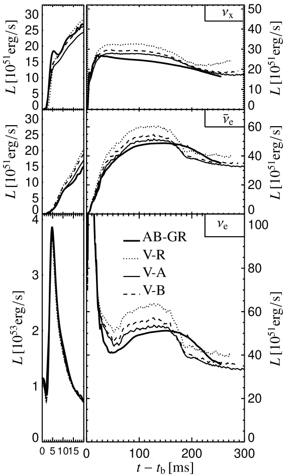
General relativistic effects are unlikely as an explanation, because they are very small around the shock (see Fig. 13 in Liebendörfer et al. 2005). A detailed analysis reveals that both codes produce internally consistent results, conserving to good precision the luminosity through the shock for an observer at rest and showing the expected and physically correct behavior in the limit of large radii. Most of the observed difference (which has no mentionable significance for supernova modeling) could be traced back to the fact that Vertex achieves only order $(v/c)$ accuracy, whereas Agile-BoltzTran produces the full relativistic result including higher orders in $(v/c)$. Corresponding effects become noticeable when $v/c\ga 0.1$. The mean neutrino energies are hardly affected by this difference (Fig. 9, bottom right panel). In case of the $\nu_{e}$ and $\bar{\nu}_{e}$ luminosities the Vertex run yields roughly 10% lower values outside of the corresponding neutrino spheres (i.e., between about $50\mathrm{\ km}$ and $90\mathrm{\ km}$), but values much closer to those from the Agile-BoltzTran calculation ahead of the shock. Since the neutrinospheric emission of $\nu_{e}$ and $\bar{\nu}_{e}$ is strongly affected by the mass accretion rate of the nascent neutron star and the corresponding accretion luminosity (which both seem to have the tendency of being slightly higher in Model AB-GR), we refrain from ascribing the different magnitude of the $\nu_{e}$ and $\bar{\nu}_{e}$ luminosities only to the treatment of relativistic effects. Although such a connection cannot be excluded, the luminosity differences might (partly) also be a consequence of the different accretion histories in Models AB-GR and V-A, which manifest themselves in the shock trajectories (Fig. 8) and are attributable to the different handling of the microphysics and computational grid in the infall layer (see above and Liebendörfer et al. 2005). This interpretation seems to be supported by the time evolution of the neutrino luminosities plotted in Fig. 10. The accretion bump in the $\nu_{e}$ and $\bar{\nu}_{e}$ luminosities which follows after the prompt $\nu_{e}$ burst is stretched in time in case of Model AB-GR, indicating the delay of mass infall at higher rates relative to all Vertex simulations. Note that the neutrino emission reacts with a time lag of some $10\mathrm{\ ms}$ (corresponding to the cooling timescale of the accretion layer on the neutron star) to variations of the mass accretion rate.

Moreover, Fig. 10 shows that our variations of the effective relativistic potential in the Vertex models have little influence on the prompt burst of $\nu_{e}$ at shock breakout. But subsequently the overestimated compactness of the proto-neutron star in Model V-R, which causes the faster contraction of the stalled shock after maximal expansion (Fig. 8), also leads to higher neutrino luminosities during the accretion phase. Consistent with the shock trajectories, Model V-A yields the closest match with the general relativistic run of Model AB-GR also for the neutrino luminosities. It is very satisfactory that the results (shock radius $r_{\mathrm{s}}$ as well as the neutrino luminosities $L$) from both simulations reveal convergence at later times when the period of massive post-bounce accretion comes to an end.

In Fig. 11 we present the radial structure at $250\mathrm{\ ms}$ after bounce for the Vertex simulations with the modifications A and B of the TOV potential, compared to the results with the TOV potential (Case R) which was already discussed in Liebendörfer et al. (2005). Note that because of the excellent agreement seen in Fig. 9, Model V-A (Case A) can also be considered as a representation of the fully relativistic run of Model AB-GR. Models V-A and V-B show results of similar quality. The little offset of the shock position (which is causally linked to the differences in all profiles) might suggest that Model V-B is slightly inferior to Model V-A in approximating relativity. This conclusion could also be drawn from the post-bounce luminosities in Fig. 10. However, caution seems to be advisable with such an interpretation, being aware of the uncertainties in the accretion phase and infall layer discussed above, and in view of the fact that the central densities (Fig. 7) and radial density profiles (Fig. 11) agree well. Moreover, the quality of the agreement at “very late” times cannot be judged, because no information is available for the behaviour of Model AB-GR after $250\mathrm{\ ms}$ post bounce, a time when the settling of the shock radius and luminosities to their post-accretion levels seems not yet over in this model (Figs. 8, 10). The TOV potential of Case R clearly produces too large infall velocities ahead of the shock (and therefore does not agree well with the kinematics of the relativistic calculation), overestimates the compactness of the forming neutron star, and thus produces too high neutrino luminosities during the simulated period of evolution (for a detailed discussion, see Liebendörfer et al. 2005). Cases A and B clearly perform better and must be considered as significant improvements for use in Newtonian simulations with an effective relativistic potential as approximations to fully relativistic calculations.

4.3 Neutron stars in equilibrium – Migration test

The supernova core collapse simulations presented in Sect. 4.1 and 4.2 are limited to a maximum core compactness $2M_{\mathrm{core}}/R_{\mathrm{core}}\sim 0.2$. In order to extend the assessment of the quality of a Newtonian simulation with an effective relativistic potential to a more strongly relativistic regime, we construct spherical equilibrium models of neutron stars using a simple polytropic EoS, $P=K\rho^{\gamma}$, with $\gamma=2$ and $K=1.455\times 10^{5}$ (in cgs units). The TOV equations are solved on a very fine grid with $10^{5}$ equidistantly spaced radial grid points using a second-order accurate Runge–Kutta integration scheme. By varying the value of the central density from $\rho_{\mathrm{c}}=1.0\times 10^{14}\mathrm{\ g\ cm}^{-3}$ to $100.0\times 10^{14}\mathrm{\ g\ cm}^{-3}$, we cover the entire range from weak to strong relativistic gravity. The density variation corresponds to compactness parameters ranging from $2M_{\mathrm{g}}/R\sim 0.02$ to $0.5$, where $M_{\mathrm{g}}$ is the total gravitational mass of the neutron star and $R$ its radius. We again point out that in spherical symmetry the assumption of CFC constitutes no approximation.

Figure 12: Mass-density diagram for spherical equilibrium neutron star models (top panel) and time evolution of the central density for the migration test from the unstable to the stable branch (bottom panel). In both graphs the behaviour of the Newtonian models computed with the modification A (dotted line) and B (long-dashed line) of the TOV potential is close to that in the relativistic case (Case GR; solid line). The Newtonian equivalent of the gravitational mass $M_{\mathrm{g}}$ (dashed line) as well as the rest mass $M_{\mathrm{r}}$ (dashed-dotted line) calculated using a regular Newtonian potential (Case N) deviate strongly from the relativistic solution (top panel). While $\rho_{\mathrm{c}}$ oscillates around its initial value $\rho_{\mathrm{c\,i}}$ for Case N (dashed line), in Case R (dashed-dotted line) the neutron star disperses to a state with $\rho_{\mathrm{c}}\ll\rho_{\mathrm{c\,f}}$ (bottom panel).

The mass-density curve of the corresponding TOV neutron star models (Fig. 12, top panel) exhibits the well-known form consisting of a stable branch at low densities and an unstable branch at high densities, where the gravitational mass $M_{\mathrm{g}}$ increases or decreases with $\rho_{\mathrm{c}}$, respectively. The two branches meet at the maximum mass. Configurations on the unstable branch are unstable to small perturbations and either collapse to a black hole or migrate to a configuration on the stable branch with the same gravitational mass but a lower central density $\rho_{\mathrm{c\,f}}<\rho_{\mathrm{c\,i}}$ (as indicated by the arrow for an exemplary configuration in the top panel of Fig. 12).

While the gravitational mass $M_{\mathrm{g}}$ and the rest mass $M_{\mathrm{r}}$ are limited in relativistic gravity (Case GR), $M_{\mathrm{g}}\simeq M_{\mathrm{r}}\simeq 1.6M_{\odot}$, regular Newtonian gravity (Case N) allows for solutions with arbitrarily high rest mass $M_{\mathrm{r}}$, which are all stable against (small) perturbations. If an (unphysical) equivalent to the relativistic gravitational mass is introduced in Newtonian gravity, $M_{\mathrm{g}}\equiv M_{\mathrm{r}}-M_{\mathrm{b}}$, where $M_{\mathrm{b}}\equiv|E_{\mathrm{b}}|$ is the mass associated with the binding energy of the self-gravitating object, we find negative values at large densities, where the binding energy becomes so large that $M_{\mathrm{b}}>M_{\mathrm{r}}$.

On the other hand, when using the modifications A and B of the TOV potential in the TOV equation for the neutron star model sequence, the corresponding curves for the TOV gravitational mass $M_{\mathrm{g}}$ in Fig. 12 agree very well with the relativistic curve (Case GR) even in the high density regime, and they show the same qualitative behaviour with an increasing and a decreasing branch. The respective mass maxima are located close to the relativistic one for both modifications of the TOV potential.

Note that for constructing equilibrium configurations using the TOV potential (Case R) is identical to solving the fully relativistic TOV equations (Case GR), and thus the results are identical. Therefore, this test is useless for predicting the quality of the TOV potential in the context of a dynamic evolution. This is different when a neutron star model from the unstable branch is allowed to evolve in time using a dynamic code. Then the (small but nonzero) finite difference discretisation errors of the numerical scheme act as perturbations of the unstable equilibrium and excite small oscillations. Depending on the numerical algorithms used in the code and the resolution of the grid, the neutron star either contracts to higher densities (and ultimately to a black hole for a simple polytropic EoS) or approaches a new equilibrium state on the stable branch after a strongly dynamical, nonlinear evolution phase. This neutron star migration scenario is a standard test of the relativistic regime with strongly dynamical evolution for numerical hydrodynamic codes with relativistic gravity (see, e.g., Font et al. 2002; Baiotti et al. 2005).

The time evolution of the central density is depicted in the bottom panel of Fig. 12 for such a migration to the stable branch, where the central density $\rho_{\mathrm{c}}$ drops from $\rho_{\mathrm{c\,i}}=49.3\times 10^{14}\mathrm{\ g\ cm}^{-3}$ to $\rho_{\mathrm{c\,f}}=8.8\times 10^{14}\mathrm{\ g\ cm}^{-3}$. Shown is the evolution for a relativistic simulation (Case GR) as well as for Newtonian simulations utilizing a regular Newtonian potential (Case N), the TOV potential (Case R), and its modifications A and B. For these simulations we again use the CoCoNuT code, whose implementation of the hybrid EoS, Eqs. (12, 13) allows one to suppress the contribution of the thermal pressure $P_{\mathrm{th}}$, in which case the hybrid EoS reduces to a polytropic one.

As expected and as observed in simulations with similar relativistic codes, in relativistic gravity (Case GR) the neutron star initially expands rapidly and its central density decreases strongly. It undershoots the stable equilibrium at $\rho_{\mathrm{c\,f}}$ and experiences several ring-down oscillations of decreasing amplitude until $\rho_{\mathrm{c}}$ approaches $\rho_{\mathrm{c\,f}}$ at late times. The modifications A and B of the TOV potential both have initial (final) states on the unstable (stable) branch of the mass-density curve which are very close to the relativistic one (Case GR). Therefore the evolution of $\rho_{\mathrm{c}}$ (starting again with the same central density $\rho_{\mathrm{c\,i}}$) is similar to the relativistic case, as shown in Fig. 12. The disagreement in oscillation amplitudes and periods can be attributed to the differences in the Newtonian and relativistic kinematics. When comparing the results of migration tests using various relativistic hydrodynamic codes (Stergioulas et al. 2003), we observe that even small variations in the numerical approach, e.g., a different coordinate choice or grid setup, or differences in the treatment of the artificial atmosphere, can have a strong impact on the detailed evolution of $\rho_{\mathrm{c}}$ from the initial to the final equilibrium state. Consequently, we consider the results obtained with the modifications A or B of the TOV potential in an otherwise Newtonian formulation to be a very good approximation of the relativistic one (Case GR).

Using regular Newtonian gravity (Case N), however, yields a totally different behaviour, because there exist no unstable configurations in that case. Thus, discretisation errors cannot trigger a migration, and the star simply oscillates around its initial equilibrium state with $\rho_{\mathrm{c}}(t)\simeq\rho_{\mathrm{c\,i}}$. On the other hand, using the TOV potential (Case R) leads to a rapid dispersion (without ring-down oscillations) of the neutron star with a final central density $\rho_{\mathrm{c}}\ll\rho_{\mathrm{c\,f}}$, which is in strong qualitative disagreement with the behaviour in relativistic gravity (Case GR). We thus conclude that in the demanding test case of a migrating spherical neutron star model, both the regular Newtonian potential (Case N) and the TOV potential (Case R) fail, while the modifications A and B of the TOV potential reproduce the relativistic result very well, both qualitatively and also quantitatively.

5 Multi-dimensional simulations with rotation

For the multi-dimensional calculations we only use the CoCoNuT code, since parameter studies with MudBath (the two-dimensional version of Vertex) are computationally too expensive when neutrino transport is included. Moreover, currently there exists no other fully relativistic two-dimensional code including neutrino transport to compare our results with. The following discussion hence focuses on purely hydrodynamic simulations using the simple matter model described in Sect. 3.1.

Figure 13: Time evolution of the central density $\rho_{\mathrm{c}}$ for the rotating core collapse models A1B3G1 (top panel), A4B1G2 (centre panel), and A2B4G1 (bottom panel), respectively. With increasing influence of rotation on the collapse dynamics, the results of the Newtonian simulations with the modifications A (dotted line) and B (long-dashed line) of the TOV potential and eventually also with the TOV potential (Case R; dashed-dotted line) move away from the relativistic result (Case GR; solid line). The central density obtained with regular Newtonian gravity (Case N; dashed line) is lowest for all three models.

Motivated by the promising results in spherical symmetry, we now apply the modified effective relativistic potentials according to Eq. (7) to simulations of rotational core collapse in axisymmetry. The initial models of the pre-collapse core are described by the same EoS parameters as the ones in Sect. 4.1 with $\rho_{\rm c\,i}=10^{10}{\rm\ g\ cm}^{-3}$, but now rotate at various rotation rates with different degrees of differential rotation. To construct these rotating equilibrium configurations, we use Hachisu’s self-consistent field method (see Komatsu et al. 1989). The initial pressure reduction to trigger the collapse and the stiffening of the EoS follows the prescription given in Sect. 4.1.

For these multi-dimensional tests we choose three rotational core collapse models as representative cases. Their evolution is influenced by the effects of rotation at various degrees (for details about the specifications of these models, see Dimmelmeier et al. 2002a). The core of Model A1B3G1 is an almost uniform rotator with a moderate rotation rate and collapses nearly spherically, forming a compact remnant immediately after core bounce. Model A4B1G2 is a very differentially rotating model, which develops considerable deviations from spherical symmetry during its evolution, but otherwise shares the qualitative bounce behavior of the previous model A1B3G1. Finally, in the multiple bounce model A2B4G1 the increase of the centrifugal forces during the contraction phase causes a series of subsequent multiple bounces at subnuclear densities. The time evolution of the central density for these three models computed relativistically (Case GR) is shown with solid lines in the top, centre, and bottom panels of Fig. 13, respectively.

In a Newtonian simulation with regular Newtonian gravity (Case N) all three models exhibit several consecutive bounces (at subnuclear densities for Models A1B3G1 and A2B4G1, and just above nuclear matter densities for Model A4B1G2), with the central density being considerably lower during the entire evolution (Fig. 13). Such a qualitative change of the collapse dynamics between a Newtonian and a general relativistic simulation of the same model was also observed in the comprehensive parameter study of rotational core collapse performed by Dimmelmeier et al. (2002b).

When applying the TOV potential (Case R) or its modifications A and B to Model A1B3G1 (top panel of Fig. 13) the outcome is similar to the situation in spherical symmetry shown in Fig. 2. Case R yields a central density noticeably higher than the one in the relativistic simulation (Case GR). For Case A the result agrees very well with the relativistic one, while for Case B the central density is too small.

As the influence of rotation increases, the ordering of the curves for Cases R, A, and B (from higher to lower $\rho_{\mathrm{c}}$) remains unaltered. However, all curves are shifted to lower densities (Fig. 13). For Model A4B1G2 the result from the Newtonian simulation with the TOV potential (Case R) matches the relativistic result (Case GR) best, which is a coincidence associated with the particular rotational state of this model. For Model A2B4G1, where the influence of rotation is stronger, the results obtained for Cases A, B, and R differ considerably from the relativistic results.

A behaviour consistent with that of these three representative models is observed for other rotational core collapse models as well. Thus, in rotational core collapse, even a Newtonian simulation with the TOV potential (Case R) yields lower central densities than the corresponding relativistic simulation (Case GR) beyond a certain rotation rate (which depends both on the initial model and on the EoS parameters).

We therefore conclude that for rotational core collapse the use of neither the modifications A and B of the TOV potential nor the (stronger) TOV potential itself (Case R) can closely reproduce the collapse behaviour of a relativistic code for all degrees of rotation. Hence, in a Newtonian code either the effective relativistic potential has to include the effect of rotation, or the collapse kinematics (and thus the hydrodynamic equations) have to be modified. However, in the latter case the advantage of a Newtonian approach over a fully relativistic formulation in terms of simplicity and computational speed may be lost.

On the other hand, we find that the qualitative dynamical behaviour of relativistic rotational core collapse models (Case GR), particularly their collapse type (regular collapse, multiple bounce collapse, or rapid collapse as introduced by Zwerger & Müller 1997) is correctly captured in a Newtonian simulation for a wide range of parameter space, if the TOV potential (Case R) or its modified versions (Cases A to D) are used. Moreover, the corresponding results agree much better with the relativistic result than that obtained from a Newtonian simulation with regular Newtonian potential (Case N). Hence, the usage of the effective relativistic potentials is an improvement of Newtonian simulations also in the case of rotational core collapse.

6 Summary and Conclusions

We investigated different modifications of the TOV potential used as effective relativistic potentials in Newtonian hydrodynamics with the aim to test their quality of approximating relativistic effects in stellar core collapse and supernova simulations. This work was motivated by a recent comparison of the neutrino radiation-hydrodynamics codes Agile-BoltzTran and Vertex used by the Oak Ridge-Basel collaboration and by the Garching group, respectively (Liebendörfer et al. 2005). While the former code is a fully relativistic implementation of neutrino transport and hydrodynamics in spherical symmetry, the latter code employs an approximative relativistic description by treating the self-gravity of the stellar fluid with an effective relativistic potential tailored from a comparison of the Newtonian and relativistic equations of motion. Otherwise Vertex solves the Newtonian equations of hydrodynamics, ignoring the effects of relativistic kinematics and space-time curvature (Rampp & Janka 2002). The comparison by Liebendörfer et al. (2005) shows very good agreement of the results from both codes for the phases of stellar core collapse, bounce and prompt shock propagation. However, it also revealed a moderate but gradually increasing overestimation of the compactness of the nascent neutron star during the subsequent accretion phase, accompanied by an overestimation of the luminosities and mean energies of the emitted neutrinos.

These systematic differences suggested that an improvement might be possible by changing the effective relativistic potential such that the strength of the gravitational field is reduced relative to the TOV potential. To this end we considered a variety of modifications (Cases A–F; see Sect. 2.2) of the TOV potential (which defines our reference Case R), and compared corresponding hydrodynamic as well as hydrostatic solutions with regular Newtonian (Case N) and fully relativistic calculations (Case GR). While some modifications did not provide any significant advantage over the TOV potential, several options for the potential were identified which allow for a much better reproduction of relativistic results with Newtonian hydrodynamics. In particular, reducing the TOV mass, Eq. (4), that appears in the expression of the TOV potential, turned out to be very successful in this respect.

For example, in Case A we introduced an additional metric factor $\Gamma<1$, Eq. (5), in the integrand of the TOV mass, and in Case B we ignored the internal energy (and all terms depending on neutrinos) in the TOV mass. In both cases not only characteristic model parameters like the central density and shock radius were in excellent agreement with relativistic simulations during all stages of the evolution including the long-term accretion phase of the collapsing core after bounce. Also the radial profiles of the hydrostatic central core as obtained in the hydrodynamic simulations were found to be very good approximations of the profiles from the fully relativistic treatment. Consequently, they are nearly consistent with solutions of the TOV equations for equal central density. Migration tests of extremely relativistic, ultradense, hydrostatic configurations from the unstable to the stable branch of the mass-density relation confirmed the good qualitative and quantitative performance of the approximation even for such a demanding test problem with a strongly dynamic transition from the initial to the final state. This suggests that the use of a modified TOV potential in an otherwise Newtonian hydrodynamics code also ensures a good reproduction of relativistic kinematics.

In addition to these purely hydrodynamic simulations with the CoCoNuT code, we performed runs including neutrino transport and compared them to relativistic calculations with the Agile-BoltzTran code of the Oak Ridge-Basel collaboration (cf. the simulations for Model G15 in Liebendörfer et al. 2005). Also in this application, the modifications A and B of the TOV potential produced a major improvement relative to the original TOV potential (Case R), for which results with the Vertex code were already presented in Liebendörfer et al. (2005). Good agreement between the relativistic and approximative treatments was seen in the transport quantities as well. The Vertex code performs well despite the fact that the approximative description takes into account only relativistic redshift in the transport but – for reasons of consistency with the Newtonian hydrodynamics code – ignores the difference between proper radius and coordinate radius. Remaining (minor) quantitative differences (below about 10% for neutrino data and even smaller for hydrodynamic quantities) are probably only partly associated with relativistic effects. We suspect that a significant contribution to these differences originates from small (but unavoidable because linked to the specifics of the employed numerical methods) discrepancies in the infall layer ahead of the shock as described by the Vertex and Agile-BoltzTran codes.

The results discussed in this paper therefore demonstrate that a very good, simple, and computationally efficient approximation to a relativistic treatment of stellar core collapse and neutron star formation in spherical symmetry can be achieved by modeling the self-gravity of the stellar plasma with an effective relativistic potential based on the TOV potential as suggested in this work. Two-dimensional axisymmetric collapse calculations (using a simple equation of state and ignoring neutrino transport) for rotating stellar cores with a wide range of conditions showed that even in this case the TOV potential and its modifications reproduce the characteristics of the relativistic collapse dynamics quantitatively well for not too rapid rotation. There is still good qualitative agreement when the rotation becomes fast, in contrast to Newtonian simulations with regular Newtonian potential (Case N), which mostly fail even qualitatively. Multi-dimensional simulations with an effective relativistic potential (which in general does not satisfy the Poisson equation), however, fulfill strict momentum conservation only for special cases of symmetry (for details, see Sect. 3.3).

Although our Cases A and B yield results of similar quality for all the test problems considered here and neither is preferred when a simple equation of state is used, the situation is more in favour of Case A when microphysics is taken into account in the equation of state. When particles can annihilate or nuclear interactions take place, rest mass energy is converted into internal energy and vice versa. In such a situation baryon number and lepton number are conserved, but not the total rest mass of the particles, and only the total (“relativistic”) energy density, $\rho+e$, is a well defined quantity, but not the individual energies. Case B therefore becomes ambiguous (see Sect. 2.2) while Case A does not suffer from such problems. We therefore are tempted to recommend using Case A as an effective relativistic potential in Newtonian hydrodynamics codes. The extra factor $\Gamma<1$ in the integrand of the TOV mass, Eq. (4), reduces the mass integral below the mass equivalent of the total (rest mass plus internal) energy. Its introduction may be justified by heuristic arguments and consistency considerations when the relativistic concept of the gravitating mass is applied in a Newtonian description of the dynamics, which does not distinguish between proper volumes and coordinate volumes (see Sect. 2.3).

Appendix A Construction of an “effective” one-parameter equation of state

The relativistic TOV solution for a spherical, self-gravitating matter distribution in equilibrium can be found by solving the following two coupled ordinary differential equations for the pressure $P$ and the mass $m$:

$$\frac{\partial P}{\partial r} = -\frac{\rho(1+\epsilon)+P}{r^{2}}\left(m+4\pi r^{3}P\right)\left(1-\frac{2m}{r}\right)^{-1}\!\!\!\!\!\!\!,$$ (14)

$$\frac{\partial m}{\partial r} = 4\pi\rho(1+\epsilon)r^{2}.$$ (15)

with appropriate boundary conditions at the inner and outer boundary at $r=0$ and $r=R$, respectively. Note that for a TOV solution the mass $m(R)$ is equivalent to the total gravitational mass $M_{\mathrm{g}}$ of the matter configuration.

The above system is closed by choosing a two-parameter EoS $P(\rho,\epsilon)$ and assuming a distribution profile for the specific internal energy $\epsilon$, which effectively transforms the EoS into a one-parameter relation, $P=P(\rho)$ [or alternatively $\rho=\rho(P)$], from which the specific internal energy can be determined as $\epsilon=\epsilon(P,\rho)$. A typical example for this is to demand a polytropic relation for $P$ and to specify the internal energy $\epsilon$ by the ideal gas EoS:

$$\begin{array}[]{l@{\quad}c@{\quad}l}P=K\rho^{\gamma},&&\displaystyle\rho=\left(\frac{P}{K}\right)^{1/\gamma}\!\!\!\!\!\!\!\!,\\[-3.00003pt] &\longrightarrow&\\[-3.00003pt] P=\rho\epsilon(\gamma-1),&&\displaystyle\epsilon=\frac{P}{\rho(\gamma-1)}.\end{array}$$ (16)

For a two-parameter EoS of the form of Eqs. (12, 13), where a priori no profile for the specific internal energy is known, the following procedure can be applied to construct an “effective” one-parameter EoS. For matter in equilibrium, e.g., at late times long after the core bounce phase, both the radial profiles of the pressure $P(r)$ and the density $\rho(r)$, as well as the specific internal energy $\epsilon(r)$ can be assumed to be stationary. If the pressure profile is monotonic, then for each value of $P$ there exists a unique location $r$. By inverting the pressure profile, $P(r)\longrightarrow r(P)$, we can thus relate a specific value $\rho(r)$ and $\epsilon(r)$ to each value of $P$. This way a one-parameter EoS $\rho=\rho(r(P))$ [and $\epsilon=\epsilon(r(P))$] can be constructed.

The excellent matching of the density profiles in the central part of a collapsed core in equilibrium obtained from a dynamic evolution with profiles from a TOV solution using equal central density and the EoS transformed as described above (see Figs. 3 to 5) demonstrates the applicability of this method.

Appendix B Radial coordinate transformation

To compare a solution of the TOV equations (14, 15), which are formulated in standard Schwarzschild-like coordinates, to results from our evolution code using relativistic gravity, which is based on radial isotropic coordinates, we must perform a coordinate transformation of the radial coordinate.

In standard Schwarzschild-like coordinates, the line element $\mathrm{d}s_{\mathrm{st}}^{2}$ reads

$$\mathrm{d}s_{\mathrm{st}}^{2}=-A\,\mathrm{d}t_{\mathrm{st}}^{2}+B\,\mathrm{d}r_{\mathrm{st}}^{2}+r_{\mathrm{st}}^{2}\,\mathrm{d}\Omega_{\mathrm{st}}^{2},$$ (17)

while the line element $\mathrm{d}s_{\mathrm{iso}}^{2}$ in radial isotropic coordinates is given by

$$\mathrm{d}s_{\mathrm{iso}}^{2}=-\alpha^{2}\,\mathrm{d}t_{\mathrm{iso}}^{2}+\phi^{4}\left(\mathrm{d}r_{\mathrm{iso}}^{2}+r_{\mathrm{iso}}^{2}\mathrm{d}\Omega_{\mathrm{iso}}^{2}\right).$$ (18)

In vacuum outside the matter distribution, the metric components become

$$A=1-\frac{2M_{\mathrm{g}}}{r_{\mathrm{st}}},\qquad B=\left(1-\frac{2M_{\mathrm{g}}}{r_{\mathrm{st}}}\right)^{-1}\!\!\!\!\!=A^{-1}$$ (19)

and

$$\alpha=\frac{1-\frac{M_{\mathrm{g}}}{2r_{\mathrm{iso}}}}{1+\frac{M_{\mathrm{g}}}{2r_{\mathrm{iso}}}},\qquad\phi=1+\frac{M_{\mathrm{g}}}{2r_{\mathrm{iso}}},$$ (20)

respectively.

As with both metrics one can describe a spherical matter distribution in equilibrium, equating the line elements, $ds_{\mathrm{st}}^{2}=ds_{\mathrm{iso}}^{2}$, yields conditions for each of the coordinates and metric components in such a case.

Setting the two coordinate times equal, we obtain a condition for $A$ and $\alpha$:

$$\left.\begin{array}[]{rcl}A\,\mathrm{d}t_{\mathrm{st}}^{2}&=&\alpha^{2}\,\mathrm{d}t_{\mathrm{iso}}^{2},\\[3.00003pt] \mathrm{d}t_{\mathrm{st}}&=&\mathrm{d}t_{\mathrm{iso}},\end{array}\right\}\quad\longrightarrow\quad\sqrt{A}=\alpha.$$ (21)

A similar condition can be obtained for the angle element:

$$\left.\begin{array}[]{rcl}r_{\mathrm{st}}^{2}\,\mathrm{d}\Omega_{\mathrm{st}}^{2}&=&\phi^{4}r_{\mathrm{iso}}^{2}\mathrm{d}\Omega_{\mathrm{iso}}^{2},\\[3.00003pt] \mathrm{d}\Omega_{\mathrm{st}}&=&\mathrm{d}\Omega_{\mathrm{iso}},\end{array}\right\}\quad\longrightarrow\quad r_{\mathrm{st}}=\phi^{2}r_{\mathrm{iso}}.$$ (22)

From the radial elements, we get a relation for the radial differentials:

$$\sqrt{B}\,\mathrm{d}r_{\mathrm{st}}=\phi^{2}\,\mathrm{d}r_{\mathrm{iso}}.$$ (23)

Knowing the solution in the isotropic radial coordinate, it is straightforward to derive a simple expression for $r_{\mathrm{st}}(r_{\mathrm{iso}})$ from Eq. (22).

On the other hand, obtaining the inverse relation $r_{\mathrm{iso}}(r_{\mathrm{st}})$ is more complicated. For this, we insert Eq. (22) into Eq. (23) and arrive at

$$\frac{\mathrm{d}r_{\mathrm{iso}}}{\mathrm{d}r_{\mathrm{st}}}=\frac{\sqrt{B}}{\phi^{2}}=\frac{r_{\mathrm{iso}}}{r_{\mathrm{st}}}\sqrt{B}.$$ (24)

This differential equation can be solved by numerical integration using, e.g., a Runge–Kutta integration scheme with the following boundary conditions:

$$r_{\mathrm{0\,iso}} = r_{\mathrm{0\,st}}=0,$$ (25)

$$R_{\mathrm{iso}} = \frac{R_{\mathrm{st}}}{2}\left(1-\frac{M_{\mathrm{g}}}{R_{\mathrm{st}}}+\sqrt{1-\frac{2M_{\mathrm{g}}}{R_{\mathrm{st}}}}\right).$$ (26)

An alternative method is to rewrite Eq. (24) in terms of $\ln r_{\mathrm{iso}}$,

$$\frac{\mathrm{d}\ln r_{\mathrm{iso}}}{\mathrm{d}r_{\mathrm{st}}}=\frac{\sqrt{B}}{r_{\mathrm{st}}},$$ (27)

which can be directly integrated numerically.

References

- Baiotti et al. (2005) Baiotti, L., Hawke, I., Montero, P. J., et al. 2005, Phys. Rev. D, 71, 024035
- Baron et al. (1989) Baron, E., Myra, E. S., Cooperstein, J., & van den Horn, L. J. 1989, ApJ, 339, 978
- Cerdá-Durán et al. (2004) Cerdá-Durán, P., Faye, G., Dimmelmeier, H., et al. 2004, A&A, in press; astro-ph/0412611
- Cook et al. (1996) Cook, G. B., Shapiro, S. L., & Teukolsky, S. A. 1996, Phys. Rev. D, 53, 5533
- Dimmelmeier et al. (2002a) Dimmelmeier, H., Font, J. A., & Müller, E. 2002a, A&A, 388, 917
- Dimmelmeier et al. (2002b) Dimmelmeier, H., Font, J. A., & Müller, E. 2002b, A&A, 393, 523
- Dimmelmeier et al. (2005) Dimmelmeier, H., Novak, J., Font, J. A., Ibáñez, J. M., & Müller, E. 2005, Phys. Rev. D, 71, 064023
- Font et al. (2002) Font, J. A., Goodale, T., Iyer, S., et al. 2002, Phys. Rev. D, 65, 084024
- Fryxell et al. (1990) Fryxell, B., Müller, E., & Arnett, D. 1990, in Proceedings of the 5th Workshop on Nuclear Astrophysics, Ringberg Castle, 30 January–4 February, 1989, ed. W. Hillebrandt & E. Müller (Garching, Germany: MPI für Astrophysik), 100
- Isenberg (1978) Isenberg, J. A. 1978, University of Maryland Preprint, unpublished
- Janka et al. (1993) Janka, H.-T., Zwerger, T., & Mönchmeyer, R. 1993, A&A, 268, 360
- Kippenhahn & Weigert (1990) Kippenhahn, R. & Weigert, A. 1990, Stellar Structure and Evolution, Astronomy and Astrophysics Library (Berlin, Germany: Springer)
- Komatsu et al. (1989) Komatsu, H., Eriguchi, Y., & Hachisu, I. 1989, MNRAS, 237, 355
- Lattimer & Swesty (1991) Lattimer, J. M. & Swesty, F. D. 1991, Nucl. Phys. A, 535, 331
- Liebendörfer et al. (2004) Liebendörfer, M., Messer, O. E. B., Mezzacappa, A., et al. 2004, ApJS, 150, 263
- Liebendörfer et al. (2001) Liebendörfer, M., Mezzacappa, A., & Thielemann, F.-K. 2001, Phys. Rev. D, 63, 104003
- Liebendörfer et al. (2005) Liebendörfer, M., Rampp, M., Janka, H.-T., & Mezzacappa, A. 2005, ApJ, in press; astro-ph/0310662
- Liebendörfer et al. (2002) Liebendörfer, M., Rosswog, S., & Thielemann, F.-K. 2002, ApJS, 141, 229
- Müller & Steinmetz (1995) Müller, E. & Steinmetz, M. 1995, Computer Phys. Commun., 89, 45
- Ott et al. (2005) Ott, C. D., Zink, B., Dimmelmeier, H., et al. 2005, in preparation
- Rampp & Janka (2002) Rampp, M. & Janka, H.-T. 2002, A&A, 396, 361
- Shapiro & Teukolsky (1983) Shapiro, S. L. & Teukolsky, S. A. 1983, Black holes, white dwarfs, and neutron stars: The physics of compact objects (New York, NY, U.S.A.: Wiley)
- Shibata & Sekiguchi (2004) Shibata, M. & Sekiguchi, Y. 2004, Phys. Rev. D, 69, 084024
- Shu (1992) Shu, F. H. 1992, The Physics of Astrophysics, Vol. II, Gas Dynamics (Mill Valley, CA, U.S.A.: University Science Books)
- Stergioulas et al. (2003) Stergioulas, N., Zink, B., & Font, J. A. 2003, private communication
- van Riper (1979) van Riper, K. A. 1979, ApJ, 232, 558
- Wilson et al. (1996) Wilson, J. R., Mathews, G. J., & Marronetti, P. 1996, Phys. Rev. D, 54, 1317
- Woosley & Weaver (1995) Woosley, S. E. & Weaver, T. A. 1995, ApJS, 101, 181
- Zwerger & Müller (1997) Zwerger, T. & Müller, E. 1997, A&A, 320, 209