A Photometric Redshift Galaxy Catalog from the Red-Sequence Cluster Survey

Abstract

The Red-Sequence Cluster Survey (RCS) provides a large and deep photometric catalog of galaxies in the $z^{\prime}$ and $R_{c}$ bands for  90 square degrees of sky, and supplemental $V$ and $B$ data have been obtained for 33.6 deg². We compile a photometric redshift catalog from these 4-band data by utilizing the empirical quadratic polynomial photometric redshift fitting technique in combination with CNOC2 and GOODS/HDF-N redshift data. The training set includes 4924 spectral redshifts. The resulting catalog contains more than one million galaxies with photometric redshifts $<1.5$ and $R_{c}<24$, giving an rms scatter $\sigma(\Delta{z})<0.06$ within the redshift range $0.2<z<0.5$ and $\sigma(\Delta{z})<0.11$ for galaxies at $0.0<z<1.5$. We describe the empirical quadratic polynomial photometric redshift fitting technique which we use to determine the relation between redshift and photometry. A kd-tree algorithm is used to divide up our sample to improve the accuracy of our catalog. We also present a method for estimating the photometric redshift error for individual galaxies. We show that the redshift distribution of our sample is in excellent agreement with smaller and much deeper photometric and spectroscopic redshift surveys.

1 Introduction

The study of the formation and evolution of large-scale structure is essential to our understanding of the universe. The typical method to measure the distances of faint galaxies is to obtain their spectroscopic redshifts. The spectroscopic method, however, is very time consuming for surveying a large area with a deep limiting magnitude, even when using a multi-object spectrograph. The less accurate photometric redshift technique has been proved to be an efficient and effective way to measure approximately the redshifts of galaxies and to study their statistical properties and evolution (e.g., Koo, 1985; Connolly, Csabai, & Szalay, 1995; Gwyn & Hartwick, 1996; Sawicki, Lin, & Yee, 1997; Hogg et al., 1998; Wang, Bahcall, & Turner, 1998; Fernández-Soto, Lanzetta, & Yahil, 1999; Benítez, 2000; Csabai, Connolly, & Szalay, 2000; Budavári et al., 2000; Rudnick et al., 2001; Csabai et al., 2003). Basically, the technique is a transformation between a set of observable parameters (e.g., magnitudes, colors) and estimates of the physical properties of galaxies (e.g., redshift, luminosity). Often the photometric redshift technique is applied to multi-color deep imaging surveys over a small area (e.g., the Hubble Deep Field, Sawicki et al. 1997 and Fernández-Soto et al. 1999; the Canada-France Deep Fields, Brodwin et al. 2003; the COMBO-17 Survey, Wolf et al. 2003; the Las Campanas Infrared Survey, Chen et al. 2003; the GOODS-S, Mobasher et al. 2004). These surveys have sufficient depth for measuring objects at high redshift ($z\gtrsim 1$), but they only probe small cosmological volumes which might not provide a representative sample of the universe due to the limited survey area. With more and more large multi-color imaging surveys, larger and statistically more complete studies of galaxies can be done. Although the application of photometric redshift techniques to the Sloan Digital Sky Survey (SDSS) covers a large sky area and provides a huge redshift sample, the photometric data are still too shallow ($r$ $<$ 21) for galaxies at $z>0.5$ (Csabai et al., 2003). The Oxford-Dartmouth Thirty Degree Survey (ODTS, MacDonald et al. 2004) has both sufficient depth and a relatively large area ($\sim$30 deg²), but it does not have a large spectroscopic training set to calibrate the photometric redshifts. A deep multicolor survey with large area and proper spectroscopic data will vastly improve on the current results.

The Red-Sequence Cluster Survey (RCS, Gladders & Yee, 2004) is a 4m-class imaging survey in the $R_{c}$ and $z^{\prime}$ bands covering $\sim 90$ deg² total in the northern and southern sky. We have obtained follow-up observations in $V$ and $B$ for a sub-area of the RCS. The four color photometry ($z^{\prime}$, $R_{c}$, $V$, and $B$) allows us to cover a relatively large sub-area (33.6 deg²) which samples a large cosmological volume for galaxies up to redshift $\sim$ 1.5. This sub-area with four-color photometry overlaps with the Canadian Network for Observational Cosmology (CNOC2) Field Galaxy Redshift Survey (Yee et al. 2000; 2005, in preparation) which provides several thousand redshifts which can be used for the empirical photometric redshift technique and provide verification of the photometric redshifts obtained. By applying an empirical quadratic polynomial photometric redshift fitting method to the RCS photometric catalogs, a photometric redshift catalog containing about one million galaxies at $z<1.5$ with relatively small redshift errors can be generated.

In this paper we describe details of the RCS follow-up $V$ and $B$ observations and the techniques used to generate the photometric redshift catalog for the RCS survey. In §2 we describe the data we used for the photometric redshift fitting and the photometric calibrations for the $V$ and $B$ data. In §3 we provide a description of the spectroscopic training sets used in the photometric redshift fits. Section 4 presents the photometric redshift technique we used. We describe the method used to estimate the photometric redshift error in §5. We then demonstrate the results and present an example of the catalog in §6. In §7 we summarize the advantage of the photometric redshift catalog from the RCS and discuss possible follow-up studies based on the catalog.

2 The Data

2.1 Observations

The RCS (Gladders & Yee, 2004) was designed to find clusters in a large volume, at high redshift, and to low masses. The primary goals are to define a large sample of galaxy clusters at $z\sim 1$, hence providing a measurement of $\Omega_{M}$ and $\sigma_{8}$, and to perform studies of the evolution of galaxy clusters using a large complete sample. Two filters ($z^{\prime}$ and $R_{c}$) were chosen to find clusters at $0.4<z<1.4$ by applying the cluster red-sequence method (Gladders & Yee, 2000). There are 19 widely separated patches in both the northern and southern sky, covering $\sim 90$ deg² in total. The northern half of the survey was observed with the CFH12K CCD camera on the 3.6m Canada-France-Hawaii Telescope (CFHT), and the southern half was obtained using the Mosaic II camera on the Cerro Tololo Inter-American Observatory (CTIO) 4m Blanco telescope. For the CFHT RCS runs, each patch consists of fifteen CFH12K pointings arranged in a slightly overlapping grid of 3 $\times$ 5 pointings. The CFH12K camera is a 12k $\times$ 8k pixel² CCD mosaic camera, consisting of twelve 2k $\times$ 4k pixel² CCDs (from MIT Lincoln Laboratories) arranged in a 6 $\times$ 2 grid. It covers a 42 $\times$ 28 arcminute² area for the whole mosaic at prime focus (f/4.18), corresponding to 0.2059 arcseconds per pixel. We note that the average East-West (X) gap between the CCDs is 7.8 arcseconds, and the average North-South (Y) gap between the CCDs is 6.8 arcseconds. The observation dates are from May 1999 to January 2001. The typical seeing is 0.62 arcsec for $z^{\prime}$ and 0.70 arcsec for $R_{c}$. The integration times are typically 1200s for $z^{\prime}$ and 900s for $R_{c}$, with average 5$\sigma$ limiting magnitudes of $z^{\prime}_{AB}=23.9$ and $R_{c}=25.0$ (Vega) for point sources, adoping an aperture of diameter 2.7 arcsec (on average). The data and the photometric techniques are described in detail in Gladders & Yee (2004).

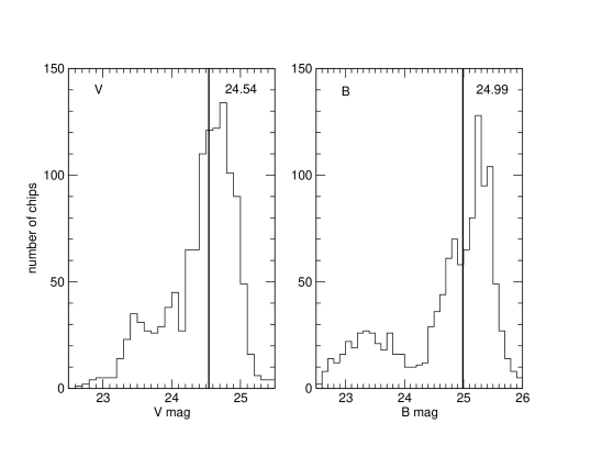
Figure 1: Histograms of $V$ and $B$ 5$\sigma$ limiting magnitudes. The distributions of 5$\sigma$ point source magnitudes from individual chips for the $V$ filter and $B$ filter are shown in the left panel and the right panel, respectively. The thick lines indicate the median value of the limiting magnitudes for $V$ and $B$, which are 24.54 and 24.99, respectively. Note that a number of pointings have very shallow $B$ limits due to observations done in poor seeing.

The follow-up observations in $V$ and $B$ were obtained using the CFH12K camera and cover 33.6 deg² ($\sim 75$% complete for the original CFHT RCS fields). The follow-up $V$ and $B$ observations contain 108 pointings spread over the ten CFHT RCS patches. The pointings of the CFHT RCS patches are shown in Table 2.1. For each pointing, a single exposure in each field was taken without dithering. The observation dates are from May 2001 to June 2002. Most data were taken in three runs in queue mode: 01AC44, 01BC25, and 02AC25. The data for another 29 pointings were taken using the observing time (run 01BC28) shared with the EXPLORE project (Yee et al., 2002). Some data were also taken during two CNOC2 photometric redshift runs using CFH12K in January 2000 and December 2000. We had 16 photometric nights out of 50 nights in which data were taken. Because some data were taken under non-photometric conditions, short exposures were obtained in photometric weather for calibration. The typical seeing is 0.65 arcsec for $V$ and 0.95 arcsec for $B$. The average exposure times for $V$ and $B$ are 480s and 840s, respectively, and the median 5$\sigma$ limiting magnitudes (Vega) for point sources are 24.5 and 25.0, respectively, with an adopted aperture of diameter 2.9 arcsec (on average). We present histograms of the $V$ and $B$ 5$\sigma$ limiting magnitudes in Figure 1.

Table 1: CFHT RCS Patches

Patch number	Patch name	RA(2000)	DEC(2000)	Area (deg2) with $R_{c}$ and $z^{\prime}$	Area with four filters	Notes
01	0226+00	02 26 07.0	+00 40 35	4.81	3.99	CNOC2 Patcha
02	0351-09	03 51 20.7	-09 57 41	4.79	4.30
03	0926+37	09 26 09.6	+37 10 12	5.59	4.85	CNOC2 Patcha
04	1122+25	11 22 22.5	+25 05 55	4.78	4.72
05	1327+29	13 27 41.9	+29 43 55	4.54	1.34	PDCS Patchb
06	1416+53	14 16 35.0	+53 02 26	4.53	3.04	Groth Strip
07	1449+09	14 49 26.7	+09 00 27	4.17	2.01	CNOC2 Patcha
08	1616+30	16 16 35.5	+30 21 02	4.26	4.16
09	2153-05	21 53 10.8	-05 41 11	3.43	2.96	CNOC2 Patcha
10	2318-00	23 18 10.7	-00 04 55	4.84	2.23

References. — ^aYee et al. (2000), ^bPostman et al. (1996)

2.2 Photometric Data Reduction

Photometric data reduction including object finding, star-galaxy classification, and aperture photometry was performed using the program PPP, described in detail in Yee (1991) and Yee, Ellingson, & Carlberg (1996).

The RCS $z^{\prime}$ and $R_{c}$ object finding and photometry were already done as part of the primary cluster finding program, and are described in detail in Gladders & Yee (2004). To simplify the photometric measurement procedure, we used the pixel positions of objects in the $R_{c}$ image to do photometry for $V$ and $B$. To achieve this, the position of each object in $V$ and $B$ must be accurately determined to within two pixels in radius relative to the $R_{c}$ image, sufficiently close for PPP to do a recentroiding of the object position before performing photometry. However, the follow-up observations in $V$ and $B$ began a semester after the observations in $z^{\prime}$ and $R_{c}$ were finished. The CFH12K CCD was taken off and re-installed on the prime focus for each run, and the camera was not at the identical position after each re-installation. Hence, the $V$ and $B$ images are rotated slightly relative to the $z^{\prime}$ and $R_{c}$ images for the same field. The telescope pointing is also not identical. To deal with these problems, we match the $V$ and $B$ images to the $R_{c}$ image before performing photometry.

Because we did not dither to make one large image per pointing, we match the images chip by chip. The transformation function between the $V$ and $B$ images and the $R_{c}$ images can be easily determined from bright reference objects. However, the new transformed coordinates for each pixel are almost always not integer numbers after applying the transformation function with non-integer shifts and rotation. Therefore re-sampling is needed. To avoid degradation of the image quality and to preserve the Poisson characteristics of the photon noise in the images, we use the nearest neighbor re-sampling algorithm, which also preserves flux. We use the closest integer coordinate of the transformed non-integer coordinate as the new coordinate for each original pixel. However, two original pixels may produce two transformed non-integer coordinates which may have the same nearest integer coordinate. In other words, one new pixel may be assigned fluxes from two original pixels because of round off in the pixel coordinates. In addition, some new coordinates may have zero flux because they are not the nearest coordinates for any original pixels. The photometry results would not be correct when either condition occurs within a photometry aperture. We try to deal with the problem by subtracting the local background from a pixel containing double fluxes because that pixel will also contain double the background counts. On the other hand, we put the counts of the local background into those pixels with zero flux. These procedures minimize the errors on the photometry. We note that on average, only approximately 500 pixels (ranging from 0 to 3,000 depending on the rotation angle) are affected for each chip. Given that the total number of objects in each chip is $\sim 5,000$ and that the average diameter of the photometry aperture is 14 pixels, we estimate that only $\sim 50$ pixels in photometry apertures are affected in each chip; i.e., only one object out of 100 is affected and the effect has been minimized by the method we described above (the magnitude difference before and after the transformation for an affected object is less than 0.02 magnitude).

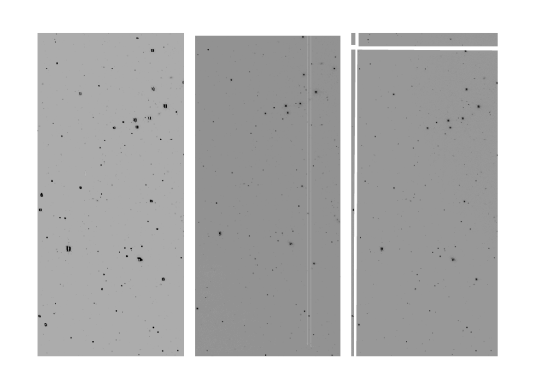
Figure 2: An example of resampled images from field 2153A1/CCD Chip07. The left image in $R_{c}$ is used as the reference image. The central image is the original (before matching) image in $V$. The right image is the shifted/rotated image in $V$ made by matching to the $R_{c}$ image. Note that the upper part and left part of the right image are copied from the nearby chips to keep the completeness of the $V$ image, and the gaps are not filled with any counts here for clarity of presentation. The bad columns in the original $V$ image are fixed for the shifted/rotated $V$ image by using a linear interpolation algorithm.

Additionally, the transformed image of each chip often overlaps with several nearby chips of the original image, and the matched regions from other chips are also cropped and included in the transformed image. We note that within each pointing, images from all the chips have been scaled to have the same zeropoint. An example of a re-sampled $V$ image is shown in Figure 2. The gaps between chips are also filled with counts of the local background. Objects falling into the gaps are lost. The final transformed $V$ and $B$ images are matched with the $R_{c}$ images for the same fields. The typical shift is between a few pixels to one hundred pixels. The typical rotation angle is about 0.03 degree and the largest angle is less than one degree.

After the matching is done, we apply the coordinate file of objects from the $R_{c}$ image to perform the aperture photometry procedure. Since the same coordinate file is used for the data in different filters, the object ID of each object in different filters of the same pointing remains the same. The multi-color photometric catalog can be generated very easily by just combining the photometric results object by object directly. The colors are measured using identical apertures for all four filters, as prescribed in Yee (1991).

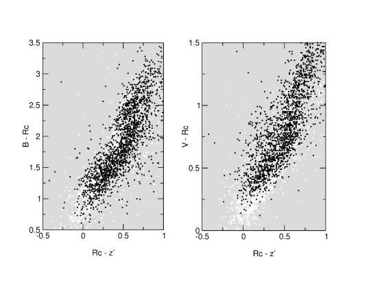
Figure 3: Color-color diagrams of 0226A3 and 0226C1. The left panel is the $B-R_{c}$ vs. $R_{c}-z^{\prime}$ diagram. The right panel is the $V-R_{c}$ vs. $R_{c}-z^{\prime}$ diagram. The white dots and black dots indicate extended sources with $R_{c}<21.5$ in 0226A3 and 0226C1, respectively. The distributions of galaxies in the two pointings in the color-color diagrams do not match, especially for $V-R_{c}$ vs. $R_{c}-z^{\prime}$. It is evident that the original photometric calibrations are not sufficiently accurate, and some additional recalibrations have to be performed.

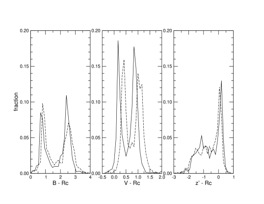
Figure 4: Color histograms of 0226A3 and 0226C1. The panels from left to right are for the colors $B-R_{c}$, $V-R_{c}$, and $z^{\prime}-R_{c}$, respectively. The solid line indicates the data from 0226A3 and the dashed line indicates the data from 0226C1. Only stars with $18<R_{c}<22$ are used. All histograms are normalized. In the three panels the color histograms for the two pointings are similar in shape but are offset from each other. By assuming that the photometric calibrations for $R_{c}$ are all correct and by choosing the pointing 0226A3 as the reference pointing, the magnitudes of $B$ and $V$ should be brighter and the $z^{\prime}$ magnitude should be a little fainter for the 0226C1 pointing. Shifts of $-0.11$, $-0.18$, and $0.09$ mag need to be applied to the $B$, $V$, and $z^{\prime}$ magnitudes, respectively, of the 0226C1 pointing in order to make the color histograms match.

The preliminary $V$ and $B$ photometric calibrations (zero-point, airmass, and color terms) were taken directly from the CFHT Elixir solutions in the image FITS file headers. The Elixir system at CFHT provides real-time data quality assessment, end-of-run detailed calibration analysis, and image pre-processing and meta-data compilation for data distribution. Data taken under bad weather conditions are calibrated by short exposures taken in photometric nights. However, we find that the color ($V-R_{c}$ or $B-R_{c}$) vs. color ($R_{c}-z^{\prime}$) diagrams have offsets from pointing to pointing, and sometimes the offsets are as large as $\sim 0.3$ magnitude, which implies that the photometric calibrations are not sufficiently accurate. An example of the differences between two pointings on the color-color diagram is shown in Figure 3. Hence, we use the following method to recalibrate the photometry. According to a recent star count study (Parker, Humphreys, & Larsen, 2003), although the densities of stars would be different for different fields, the normalized color distributions for bright stars are very similar from field to field as long as the selected fields are sufficiently large. Based on this result, we recalibrated the $z^{\prime}$, $V$, and $B$ photometry by using the $z^{\prime}-R_{c}$, $V-R_{c}$, and $B-R_{c}$ color distributions, assuming that the photometry of $R_{c}$ calibrated by standard stars is correct (Gladders & Yee, 2004). Stars with $18<R_{c}<22$ are selected to determine the magnitude offsets on a pointing-to-pointing and patch-to-patch basis. Figure 4 represents an example of the difference between the color histograms of two pointings. For the pointing-to-pointing recalibration within each patch, the pointing with the least scatter in the color-color diagrams ($V-R_{c}$ or $B-R_{c}$ vs. $R_{c}-z^{\prime}$) is chosen to be the reference pointing. (The reference pointings are 0226A3, 0351C1, 0926B4, 1122C5, 1327B2, 1416C1, 1449B2, 1616C5, 2153A1, and 2318B1 for the 10 patches.) The magnitude offsets in $z^{\prime}$, $V$, and $B$ are computed using cross-correlation of the distributions of $z^{\prime}-R_{c}$, $V-R_{c}$, and $B-R_{c}$, respectively, between the reference pointing and the test pointing. The patch-to-patch photometry recalibrations are performed after the pointing-to-pointing recalibrations are done. Patch 0926 is chosen to be the reference patch. The same recalibration procedure as the pointing-to-pointing recalibration is applied to the patch-to-patch recalibration, and all the pointings from each patch are used during the patch-to-patch recalibration procedure.

We compare the recalibrated photometry of galaxies with the overlapping published SDSS database as a check on our recalibration procedure. Patches 0226, 2318, 0926, 1416, 1449, and 1616 overlap with the SDSS Data Release 3 (DR3; Abazajian et al., 2005, http://www.sdss.org/dr3/). We match the objects between RCS and SDSS, and use the following equations to determine the relation between the two different photometry systems:

$$B=g+slope_{B}(g-r)+\Delta{B}$$

$$V=g+slope_{V}(g-r)+\Delta{V}$$

$$R_{c}=r+slope_{R_{c}}(r-i)+\Delta{R_{c}}$$

$$z^{\prime}=z+slope_{z^{\prime}}(r-i)+\Delta{z^{\prime}},$$ (1)

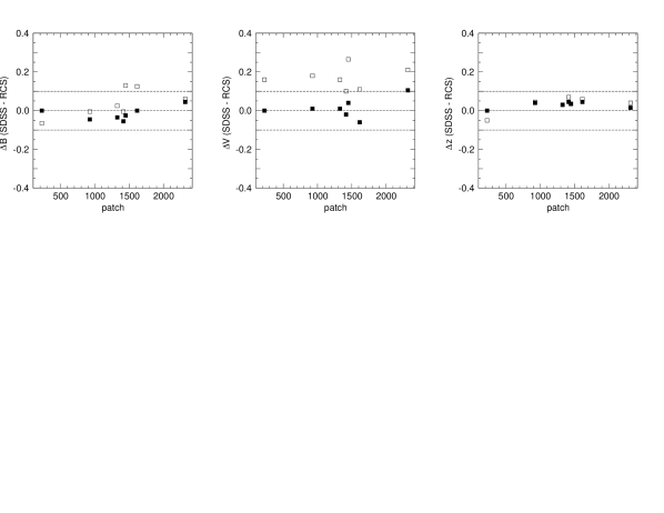
Figure 5: The zeropoint differences $\Delta$mag between RCS and SDSS in $B$, $V$, and $z^{\prime}$ (left to right) for overlapping patches; see text for details. We arbitrarily set $\Delta$mag $=0$ for patch 0226 after recalibration. Note that we do not calibrate the RCS photometry to the SDSS photometry. The open boxes and filled boxes indicate the Elixir-calibrated results and the recalibrated results, respectively. The recalibrated results show less scatter than the Elixir-calibrated ones.

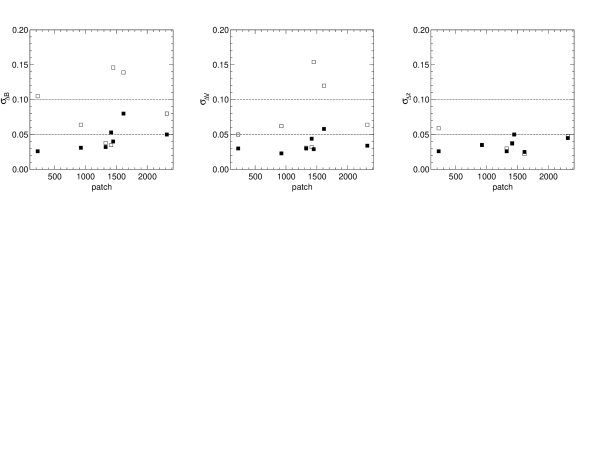
Figure 6: The standard deviations of the zeropoint difference $\Delta$mag between RCS and SDSS for the set of pointings within each RCS patch; see text for details. $B$, $V$, and $z^{\prime}$ are shown (left to right). The open boxes and filled boxes indicate the Elixir-calibrated results and the recalibrated results, respectively. The inter-pointing recalibrations for each patch reduce the standard deviations for $V$ and $B$ significantly.

where the $slope$ term is the coefficient of the color term in the transformation, and $\Delta$mag, where mag $=B,V,R_{c},z^{\prime}$, is the magnitude zeropoint difference between the RCS and SDSS photometry systems. We compare RCS magnitudes against SDSS model magnitudes. The quality of the recalibration can be verified by checking the consistency of the $\Delta$mag values between different RCS patches. In Figure 5 we plot $\Delta$mag for $B$, $V$, and $z^{\prime}$ for those RCS patches overlapping the SDSS, where we have arbitrarily set $\Delta$mag $=0$ for patch 0226 after recalibration. For these patch-to-patch comparisons we have ignored the slope terms above and simply set $\Delta$mag to the median offset between the respective RCS and SDSS magnitudes for each patch. The open boxes indicate $\Delta$mag using Elixir calibrations, and the filled boxes indicate $\Delta$mag after recalibration. The recalibrated data have less scatter between patches than the Elixir-calibrated data in all the panels, especially for $B$. Figure 6 shows the standard deviations of the $\Delta$mag values for $B$, $V$, and $z^{\prime}$ among the different pointings within each RCS patch. Here we first fit the above transformation equations to each patch as a whole, transform the SDSS magnitudes accordingly, and then compute the median offset between RCS magnitudes and transformed SDSS magnitudes for each pointing within a patch. The standard deviations of these pointing-by-pointing offsets are plotted in Figure 6. The open boxes and the filled boxes again indicate the Elixir-calibrated results and the recalibrated results, respectively. The pointing-to-pointing recalibrations reduce the standard deviations dramatically for $V$ and $B$. This RCS-SDSS comparison proves that recalibration using the color distributions of bright stars significantly improves the calibrations of the $V$ and $B$ photometry over the original Elixir-based calibrations, and that most of the original photometric calibrations (as performed by RCS, Gladders & Yee 2004) for $z^{\prime}$ are already good.

Galactic extinction has to be applied to the data before doing photometric redshift fitting. The extinction values are calculated according to prescriptions from Cardelli, Clayton, & Mathis (1989), O’Donnell (1994), and Schlegel, Finkbeiner, & Davis (1998). The galactic extinction values for the four filters for each patch are shown in Table 2. Note that our procedure will tend to result in slightly wrong galactic extinction corrections for the $B$, $V$, and $z^{\prime}$ filters, since the stars used in the recalibration procedure already suffer extinction to some extent and the recalibration procedure will have corrected for some of the extinction differences among the patches. However, the error we make is reduced because we use colors in the recalibration and because we use relative shifts among the patches. For example, if we assume that the stars we use already suffer the full amount of galactic extinction, then for patch 2318, which has the largest $E(B-V)$ value, we would have made only errors of -0.049, -0.022, and 0.024 mag for $B$, $V$, and $z^{\prime}$, respectively. Moreover, the comparison against SDSS data described above and shown in Figure 5 indicates that the extinction of stars does not cause large errors in our recalibration procedure.

Table 2: Galactic Extinction

patch name	0226	0351	0926	1122	1327	1416	1449	1616	2153	2318
E(B-V)	0.036	0.043	0.012	0.018	0.012	0.010	0.029	0.038	0.035	0.044
$A_{B}$	0.140	0.165	0.048	0.068	0.046	0.037	0.112	0.146	0.135	0.167
$A_{V}$	0.108	0.127	0.037	0.053	0.035	0.028	0.086	0.113	0.105	0.129
$A_{R_{c}}$	0.083	0.098	0.029	0.040	0.027	0.022	0.066	0.087	0.080	0.099
$A_{z^{\prime}}$	0.053	0.063	0.018	0.026	0.018	0.014	0.043	0.056	0.052	0.064

3 Spectroscopic Training Sets

Since we use an empirical quadratic polynomial fit to estimate photometric redshifts for the RCS data, we need spectroscopic data which overlap with the RCS fields to create a training set. We primarily use the spectroscopic data from the CNOC2 project, but we also include GOODS/HDF-N data to improve the limiting magnitude and redshift range of the training set. All the data included in our training set are described in detail below.

3.1 CNOC2

The Canadian Network for Observational Cosmology (CNOC2) Field Galaxy Redshift Survey (Yee et al. 2000; 2005, in preparation) is a spectroscopic/photometric survey of faint galaxies. There are four widely separated patches named 0226, 0926, 1449, and 2153. The data were obtained using the Multi-Object Spectrograph on the CFHT. The survey covers over 1.5 deg² of sky with a total sample of $\sim 6200$ redshifts with $R_{c}\lesssim 22$. The CNOC2 survey used a band-limiting filter for the spectroscopic observations to increase the number of objects observed. This produces an effective redshift range for the statistically complete sample of 0.12-0.55, and 0.0-0.68 for emission-line galaxies. The nominal statistical completeness magnitude is $R_{c}=21.5$, but there are objects as faint as $R_{c}\sim 22.5$ in the redshift sample.

Fifteen RCS pointings, distributed over four RCS patches and including four-filter photometric data, overlap the CNOC2 fields. We match the objects from the two surveys and create a training set containing the photometric data from the RCS and the spectroscopic redshifts from CNOC2. There are 3,130 objects in this training set.

3.2 GOODS/HDF-N

Compared to the spectroscopic limit of CNOC2, the photometric data of RCS are much deeper (100% completeness limit $R_{c}\simeq 24.2$ for RCS compared to the spectroscopic completeness limit $R_{c}=21.5$ for CNOC2). Furthermore, the CNOC2 spectroscopic sample has a nominal redshift limit of $\sim$ 0.55 due to the use of a band-limiting filter, and so does not provide a good training set for objects with $R_{c}\lesssim 21.5$ at $z\gtrsim 0.6$. A deeper dataset (limiting magnitude of $R_{c}\sim 24.0$) with higher redshifts ($z>0.6$) is thus needed in addition to the original training set to improve redshift estimates for high-$z$ objects in the RCS. Thus, we choose the GOODS/HDF-N data to be the additional training set for high-$z$ and fainter objects.

The Great Observatories Origins Deep Survey (GOODS; Giavalisco et al., 2004) is a survey based on multi-band imaging data obtained with the Hubble Space Telescope (HST) and the Advanced Camera for Surveys (ACS). It covers two fields (HDF-N and CDF-S) with roughly 320 arcmin² total area. For our high-redshift, faint-magnitude training set, we use publicly available $BVRz^{\prime}$ photometry and spectroscopic redshifts for the GOODS/HDF-N field. The photometry comes from the ground-based Hawaii HDF-N data set of Capak et al. (2004), which was obtained with the Subaru 8.3m telescope and has 5$\sigma$ limiting magnitudes $B_{AB}=26.9$, $V_{AB}=26.8$, $R_{AB}=26.6$, and $z^{\prime}_{AB}=25.4$ measured in 3” diameter apertures, and typical integration times of 600s, 1200s, 480s, and 180s/240s, respectively. The spectroscopic redshift data for the GOODS/HDF-N field are from the samples of Wirth et al. (2004) and Cowie et al. (2004), obtained using the Keck 10m telescope.

After combining and matching objects in the Hawaii HDF-N photometric catalog to the GOODS/HDF-N spectroscopic catalog, a training set containing 1,794 objects is generated. This additional training set is not only deeper than the RCS+CNOC2 set, but it also contains many more objects with higher redshifts ($0.5<z<1.5$). To combine the CNOC2 and GOODS training sets, we also need to offset the magnitudes of the GOODS data to match the zero-points of the RCS data. We did not use stars to derive the magnitude offsets because the field is too small to contain a statistically sufficient number of stars for the purpose. We first apply galactic extinction corrections to the GOODS/HDF-N data ($-0.018$, $-0.028$, $-0.036$, and $-0.047$ for $z^{\prime}$, $R_{c}$, $V$, and $B$), and then compute the difference in the color distributions for galaxies with $R_{c}<21.5$ between the RCS and GOODS/HDF-N samples. By assuming $R_{c}$ is always correctly calibrated, the magnitude offsets for $z^{\prime}$, $V$, and $B$ can be determined. Magnitude offsets $-0.1$, $-0.05$, and $0.0$ for $z^{\prime}$, $V$, and $B$, respectively, are applied to the GOODS/HDF-N data. The final training set created by combining the RCS+CNOC2 and the GOODS/HDF-N data includes 4924 objects. This combined training set will improve the accuracy of photometric redshifts, especially for objects at fainter magnitudes and higher redshifts.

4 Photometric Redshift Method

Photometric redshift techniques have been developed for decades (e.g., Koo, 1985), but there are two primary approaches to estimating the photometric redshift. One way is to compare the photometric data against templates generated from models or from a real spectral energy distribution database (e.g., Hogg et al. 1998; Fernández-Soto et al. 1999). The other way is to find the empirical relation between the photometric data and the redshift identified from the spectroscopic data, e.g., empirical polynomial fitting (Connolly et al. 1995). The empirical method is especially effective (e.g., see Csabai et al. 2003) when there is a large spectroscopic redshift data set available, as in the case of our RCS data set.

We use empirical quadratic polynomial fitting to estimate photometric redshifts for the RCS data. First we need to generate a subset called a “Training Set,” which includes information on object ID, spectral redshift, and photometric data for each filter (see Section 3). We then fit this subset with the following second order equation using least-squares fitting:

$$redshift=const+{a_{0}}B^{2}+{a_{1}}V^{2}+{a_{2}}{R_{c}}^{2}+{a_{3}}z^{\prime 2}$$

$$+{b_{0}}B+{b_{1}}V+{b_{2}}{R_{c}}+{b_{3}}z^{\prime}+{c_{0}}BV$$

$$+{c_{1}}B{R_{c}}+{c_{2}}Bz^{\prime}+{c_{3}}V{R_{c}}+{c_{4}}Vz^{\prime}+{c_{5}}{R_{c}}z^{\prime}.$$ (2)

Including the constant term, 15 parameters are derived from the fit. The above formula describes the empirical relation between the photometric data and the spectroscopic redshift. By applying this formula to the photometric data of an object, an estimated photometric redshift for that object is readily obtained.

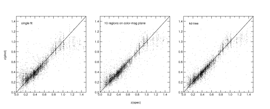
Figure 7: Photometric redshift vs. spectroscopic redshift for the RCS/CNOC2 and GOODS/HDF-N data in our training set. The panels from left to right use: (1) brute force single fit for all data, (2) cutting into 10 regions in the color-magnitude plane, and (3) the kd-tree method with 32 cells. The result using the kd-tree method has the least systematics at both the high-$z$ and low-$z$ ends, as well as the least scatter of the three methods.

One can use a brute-force single fit for all the data, but fitting all galaxies with a single quadratic formula is not optimal, since different types of galaxies may have different fitting parameters in the quadratic formula. The single fit method gives a result with large scatter and systematic deviations (see left panel, Figure 7). To improve the photometric redshift results, different types of galaxies should be fit separately. We describe below two methods of separating galaxies into different samples.

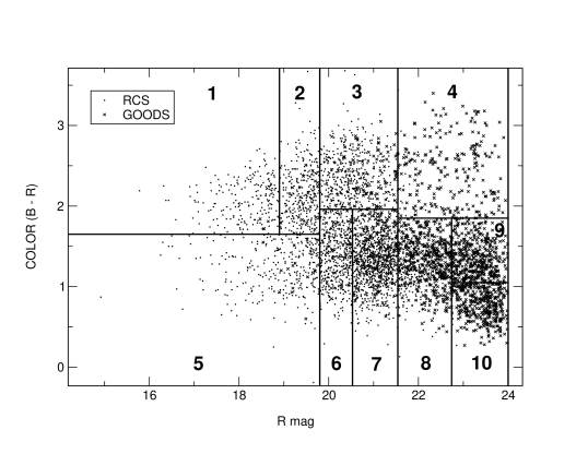
Figure 8: Color ($B-R_{c}$) vs. magnitude ($R_{c}$) diagram showing the layout of the regions used for the data separation. The dots indicate the RCS+CNOC2 data and the crosses indicate the GOODS/HDF-N data in our training set. The galaxies are roughly in two loci on the color-magnitude plane with a gap around $B-R_{c}$=1.8 to 2.0. The early-type galaxies dominate the redder (upper) locus while the late-type galaxies dominate the bluer (lower) locus. We separate the upper locus into four regions (1, 2, 3, and 4) and the lower locus into six regions (5, 6, 7, 8, 9, and 10) for the photometric redshift fits. Note that this cutting method is not used for the final catalog.

Color is one of the important signatures for identifying the galaxy type. However, it is subject to K-corrections for galaxies at different redshifts. Thus, other parameters have to be used to break the color-redshift degeneracy. Roughly speaking, more distant galaxies have fainter magnitudes, and for a reasonable range of galaxy types, they also have redder observed colors. Hence by using some appropriate boundaries to divide galaxies in the color-magnitude plane, we can mimic very roughly the effect of separating galaxies of different types at different redshifts. Figure 8 presents a color ($B-R_{c}$) vs. magnitude ($R_{c}$) diagram. The sample data consist of RCS+CNOC2 (dots) and GOODS (crosses) galaxies with $R_{c}<24$ in our training set (see §3 for a detailed description of the training set). There is a gap around $B-R_{c}$=1.8 to 2.0 which roughly separates early-type galaxies (redder) and late-type galaxies (bluer). We divide the color-magnitude plane into ten parts. Regions 1-4 are for redder galaxies, and region 5-10 are for bluer galaxies. This method produces a result with smaller scatter and systematic deviations than the single fit method (middle panel, Figure 7). However, the $B-R_{c}$ color uses filters that are too blue to make a good separation for galaxies with redshifts larger than 0.6, where the 4000Å break will be shifted to $>$ 6500Å. To solve this problem, a redder filter ($z^{\prime}$) has to be used in the separation criteria to produce a better result.

In our second method of separating the training set, we add one more color ($R_{c}-z^{\prime}$) to the original two-dimensional color-magnitude plane to form a three-dimensional color-color-magnitude space. The kd-tree algorithm, which uses median values to divide up the data points in a k-dimensional space successively (Bentley, 1979), is used to separate galaxies in our three-dimensional space. We use a kd-tree depth of five, so that the space is separated into 32 cells. Each cell contains about 150 objects. The photometric redshift fitting procedure is applied to each cell separately. We tried other numbers of cells, and they give similar results. In general, using a larger number of cells gives slightly better fits, but we choose 32 cells as a compromise so as not to be in danger of overfitting (i.e., having too few objects per cell for a 15-parameter fit). The three-dimensional kd-tree method gives a better result than the method of cutting the color-magnitude plane into 10 regions (see right panel, Figure 7).

Figure 7 compares the quality of the photometric redshifts obtained using the three different cutting methods described above. The panels from left to right are the photometric redshift vs. spectroscopic redshift diagrams obtained using: (1) brute force single fit for all data, (2) cutting into 10 regions in the color-magnitude plane, and (3) the kd-tree method with 32 cells. Both the high-$z$ and low-$z$ ends are improved with much reduced systematics as we go from method (1) to method (3). The scatter in the differences between photometric and spectroscopic redshifts is reduced as more advanced cutting algorithms are used. Hence, we choose the three-dimensional kd-tree algorithm with 32 cells for our final photometric redshift catalog.

5 Photometric Redshift Error

By examining the distribution of the differences between spectroscopic redshifts and photometric redshifts for the training set, we can estimate the uncertainty in the redshift fits. However, this does not provide a measurement of the photometric redshift error for individual galaxies in the catalog. Knowing the confidence limits on the photometric redshift measurements for individual objects is very important for subsequent science analyses. Without the confidence limits for each object, the analyses based on the photometric redshift may suffer from catastrophic errors, which happen when the photometric redshift estimates are unknowingly very different from the true spectroscopic redshifts. By considering the photometric redshift error for each object and taking it into account in estimating the errors in a subsequent science analysis, one will obtain more realistic confidence limits in the analysis results. In the following subsections, we describe the photometric redshift error determined by comparing the photometric redshifts to the spectroscopic redshifts in our training set (empirical error), and we also describe the method we use to estimate the photometric redshift error for individual objects (computed error).

5.1 Empirical Error

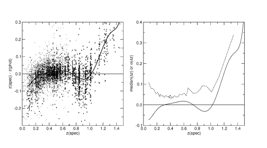
Figure 9: $\Delta{z}$ vs. spectroscopic redshift diagram (left), and median($\Delta{z}$) or $\sigma(\Delta{z})$ vs. spectroscopic redshift diagram (right) before noise is added. The fitting uses the kd-tree 32-cell cutting of the training set. The dots indicate the RCS/CNOC2 data, the crosses indicate the GOODS/HDF-N data, and the solid curve in the left panel is the median value of $\Delta{z}$. The same solid curve is also shown in the right panel for clearer presentation. The dashed curve in the right panel is the $\sigma(\Delta{z})$ which indicates the 68th percentile difference between the photometric redshift and the spectroscopic redshift, in bins of 100 objects each along the spectroscopic redshift axis. The $\sigma(\Delta{z})$ for objects at our median redshift is less than 0.05. The error becomes larger ($\sim 0.09$) for objects at $z\sim 0.9$. The extremely large error for objects at $z>1.1$ is due to the large systematic deviations at those high redshifts.

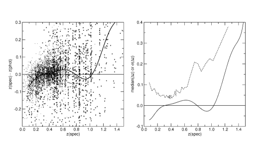
Figure 10: This figure is the same as Figure 9 but noise has been added to the GOODS/HDF-N sample (see text). The $\sigma(\Delta{z})$ for objects at our median redshift is similar compared to that in Figure 9, but the error increases to around 0.2 for objects at $z>0.8$, which is much larger than the value from Figure 9.

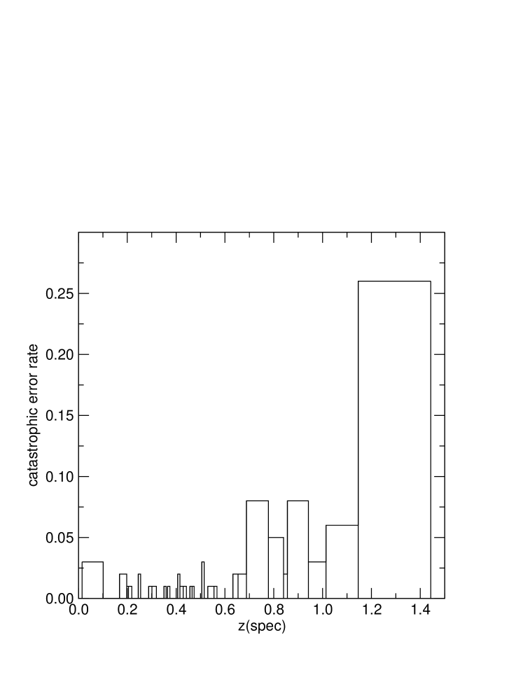
Figure 11: Histogram of catastrophic error rate vs. spectroscopic redshift. We define the catastrophic error rate as the ratio of the number of objects with $\mid\Delta{z}\mid>0.5$ to the total number of objects for each redshift bin. The result is calculated using the RCS/CNOC2 and noise added GOODS/HDF-N data. Note that the histogram has variable redshift bin widths because we choose widths that always include exactly 100 objects per bin. The catastrophic error rate is below 0.03 for $z<0.7$. It becomes around 0.05 for $0.7<z<1.2$ due to larger $\sigma(\Delta{z})$. For redshifts higher than 1.2, the catastrophic error rate is 0.25, which is primarily due to the larger systematic error.

Figure 9 presents the accuracy of the photometric redshifts by comparing the photometric redshift and the spectroscopic redshift for the objects in the training set. The $\sigma(\Delta{z})$ is the 68th percentile difference between the photometric redshift and the spectroscopic redshift in bins of 100 objects each along the spectroscopic redshift axis. This provides a general estimate of how statistically accurate our photometric redshift measurements are. For objects at $0.20<z<0.65$, the rms scatter $\sigma(\Delta{z})$ is less than 0.05. The overall rms scatter is 0.068. However, most objects at $z>0.7$ in the training set are from the GOODS/HDF-N sample, which have a much deeper limiting magnitude. The photometric redshift error for an object in the RCS at high-$z$ is thus under-estimated by the $\sigma(\Delta{z})$ of the training set. By adding additional Gaussian noise to the GOODS/HDF-N data, we simulate the photometric redshift error as if the GOODS/HDF-N data have the same depth and seeing conditions as the RCS data. The results are shown in Figure 10. For objects at $0.2<z<0.5$, the rms scatter remains roughly the same, but it becomes $\sim 0.2$ for an object at $z\sim 0.8$. The extremely large rms for objects at $z>1.1$ is caused by the large systematic deviation of the photometric redshifts from the spectroscopic redshifts. The overall average rms scatter is 0.11. This result shows the real error levels in the photometric redshift catalog. We also calculate the catastrophic error rate for different redshift ranges in bins of 100 objects each and show the result in Figure 11. We define the catastrophic error rate as the ratio of the number of objects with $\mid\Delta{z}\mid>0.5$ to the total number of objects for each redshift bin. The result is calculated using the RCS/CNOC2 and noise added GOODS/HDF-N data. Note that the histogram has variable redshift bin widths because we choose widths that always include exactly 100 objects per bin. The catastrophic error rate is below 0.03 for $z<0.7$. It becomes around 0.05 for $0.7<z<1.2$ due to larger $\sigma(\Delta{z})$. For redshifts higher than 1.2, the catastrophic error rate is 0.25, which is primarily due to the larger photometric redshift systematic error.

5.2 Computed Error

Basically the photometric redshift uncertainty for an individual object comes from two sources. One source is the error in the photometric data themselves, and the other source is the uncertainty in the empirical fitting parameters in the quadratic formula. As described below, we will use the combination of a Monte-Carlo method and a bootstrap method to estimate the effect of both these error sources and thereby compute the total photometric redshift error for each object. We refer to this error as the “estimated” or “computed” error.

The measurement error of the photometry is estimated from two sources. One is from the uncertainty of the sky measurement; the other is from the internal error of the magnitude measurement. The photometry errors are given by PPP (Yee, 1991). The Monte-Carlo method provides a way to estimate how the photometric errors statistically propagate into the error on the photometric redshift. By assuming that the distribution of the photometric uncertainties is Gaussian, we generate 500 photometric measurements, using a normal distribution with a width equal to the photometric error and centered on the original magnitude in each filter. For the estimates of the uncertainties in the photometric redshift fitting parameters (Equation 4), the training set is bootstrap-resampled 500 times to generate 500 bootstrapped training sets and corresponding solutions. By combining 500 simulated photometric data sets with 500 bootstrapped training sets, 250,000 photometric redshift estimates are produced for each galaxy. The median value of these 250,000 redshifts is chosen to be the photometric redshift of the galaxy, and the 68% width ($\sim\mbox{{1}$\sigma$}$ if the photometric redshift error distribution is Gaussian) is the estimated photometric redshift error. Note that the photometric redshift error distribution is not necessarily Gaussian. Our computed error estimate is intended to cover the 68% error range, regardless of the shape of the photometric redshift error distribution.

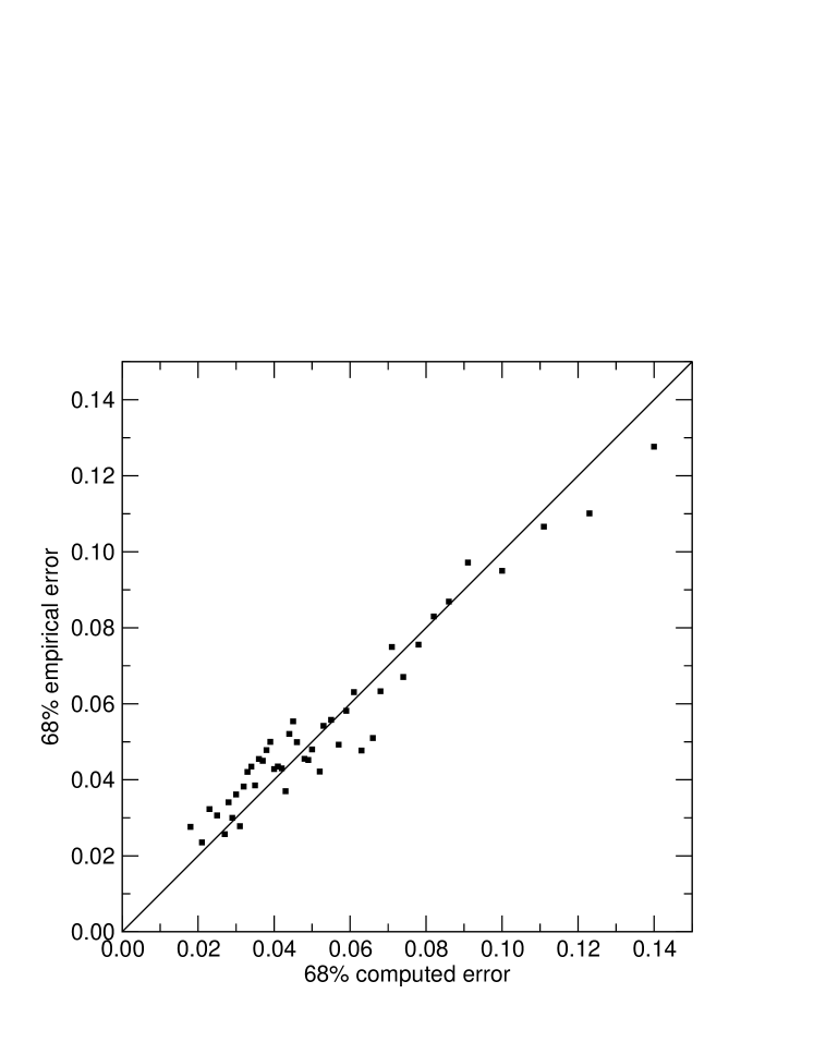
Figure 12: The empirical error vs. the computed error for RCS and GOODS/HDF-N data in our training set. The empirical error is the 68th percentile difference between the photometric redshift and the spectroscopic redshift, in bins of 100 objects each along the 68% estimated error axis. The computed error of the data point is the median value of the computed errors in the same bin of 100 objects. The computed errors agree with the empirical errors very well.

To test the quality of our photometric redshift error estimates, we compare the computed errors with the empirical errors for the galaxies in the training set. Figure 12 shows the comparison of the empirical error and the computed error for the RCS and GOODS/HDF-N data in our training set. The empirical error plotted is the 68th percentile difference between the photometric redshift and the spectroscopic redshift, in bins of 100 objects each along the 68% computed error axis. The computed error plotted is the median value of the computed errors of objects in the same bin of 100 objects. The computed errors agree very well with the empirical errors, with $\mid$empirical error - computed error$\mid\sim 0.01$. This near exact agreement of the empirical and computed error is fortuitous. When different methods of separating the training set are used, in general there is an offset and/or scaling of the computed error relative to the empirical error. However, in general, regardless of the exact fitting algorithm used, the computed errors are always well-behaved linear functions of the empirical error, showing that our method of estimating individual errors is robust.

6 Result

To produce the final photometric redshift catalog, we use the 32-cell kd-tree cutting method. From Figure 10, for objects at $0.2<z<0.5$, the rms scatter of $\Delta{z}$ is less than 0.06. For objects at $z>0.8$, the rms scatter of $\Delta{z}$ is $\sim 0.2$. The overall average rms scatter is 0.11. It can be seen that objects with lower spectroscopic redshifts are over-estimated while objects with higher spectroscopic redshifts are under-estimated (Figure 10). The bluest filter for the RCS is $B$(4500Å) and it is not blue enough for the 4000Å break at $z<0.2$. This creates a poor redshift estimate for low-z ($z<0.2$) objects, and they tend to have higher photometric redshifts than real redshifts because their SEDs and the SEDs of objects at $0.2<z<0.3$ are very similar. For those objects with redshift higher than 1.2, the 4000Å break is moving out of the reddest filter ($z^{\prime}$). A behavior opposite to the low-z objects is seen for the high-$z$ objects, i.e., they tend to have lower photometric redshifts than real redshifts.

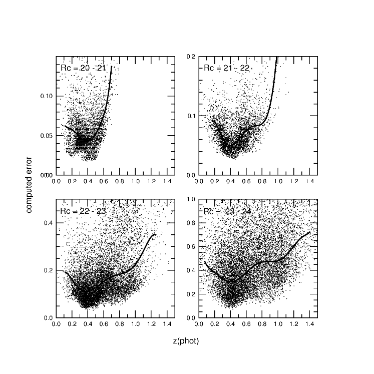
Figure 13: Computed error vs. photometric redshift in different $R_{c}$ bins. We plot a dot for every 15 and 20 objects for the $R_{c}=20-21$ and $R_{c}=21-22$ bins, respectively. For the panels with $R_{c}=22-23$ and $R_{c}=23-24$ bins, we plot a dot for every 30 and 50 objects, respectively. The curve in each panel is the median value for all data points in each $R_{c}$ bin, not just for the data shown in the figure. Note that we use different scales for the computed error axes in each panel. The error grows with fainter $R_{c}$ and higher redshift. For the objects at $z<0.25$, the errors also become larger because we do not have a sufficiently blue filter for low redshift galaxies. Generally speaking, the photometric redshift error increases with magnitude due to larger photometric uncertainty.

We present the computed error vs. photometric redshift in different $R_{c}$ bins in Figure 13. For the panels with $R_{c}=20-21$, we plot a dot for every 15 objects. For the panel with $R_{c}=21-22$, we plot a dot for every 20 objects. For the panel with $R_{c}=22-23$, we plot a dot for every 30 objects, and for the panel with $R_{C}=23-24$, every 50 objects. The curve in each panel is the median value for all the data points in each $R_{c}$ bin, not just for the data shown in the figure. Note the different scales for the computed error axes in each panel. In general, for galaxies with $R_{c}<22$ with photometric redshift less than 0.8, the errors are below 0.1. For objects with $R_{c}=22-23$, the errors become larger but there are still a significant number of galaxies with errors less than 0.1. For objects with $R_{c}=23-24$, the photometric redshift errors are greater than 0.3, which is due to larger photometric errors and also to a higher fraction of late-type galaxies. Generally speaking, the photometric redshift error increases with magnitude due to larger photometric uncertainty.

Although the galaxies are fit separately in several color and magnitude bins, the rms scatter for bluer galaxies is still much larger than the scatter for redder galaxies (shown in Figure 14). This is because early-type (redder) galaxies have some significant spectral features (e.g., the 4000Å break) and have similar SEDs, while late-type (bluer) galaxies tend to have a featureless and relatively flat continuum. Ongoing star formation, gas absorption/emission, and dust extinction will also complicate the SEDs of late-type galaxies, and different galaxies have different combinations of these effects. Because different late-type galaxies have weaker features and larger variation in their SEDs than early-type galaxies, the errors in the photometric redshift estimates will be larger for late-type galaxies.

We compare the photometric redshift technique we use to other techniques described in Csabai et al. (2003). They use nine different methods including template fits and empirical fits to estimate photometric redshifts for the SDSS Early Data Release. From their study, in general, the results using empirical fits have smaller $\sigma(\Delta{z})$ than the ones using template fits, and the best algorithm with the smallest $\sigma(\Delta{z})$ among the empirical fits is also the kd-tree method. However, the kd-tree method they use is a two-dimensional tree to cut their training set in a color-color plane, unlike what we use, which is a three-dimensional tree in a color-color-magnitude space. The addition of magnitudes provides a rough estimate of redshift which makes the separation of the training set more precise than using just colors. Combining deeper photometry, a larger training set over a wide redshift range, and a better cutting method for the training set, the limiting magnitude of our photometric redshift result is $1.5-2.0$ magnitudes deeper than the SDSS result, even with only four wide-band filters (compared to five filters for SDSS) and a much higher redshift limit. However, qualitatively, the agreement between spectroscopic and photometric redshift is similar between the SDSS and the RCS; e.g., the very low redshift galaxies tend to have over-estimated photometric redshifts.

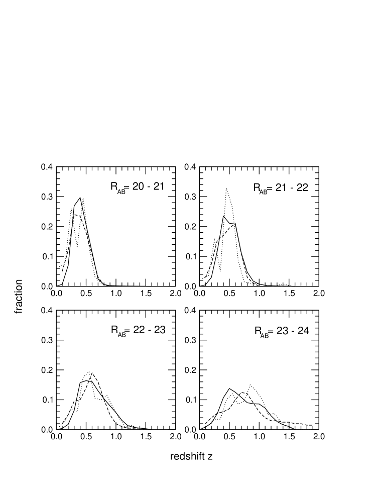
Figure 15: The redshift distribution comparison diagrams. The solid lines, dashed lines, and dotted lines indicate RCS photometric redshift, CFDF photometric redshift, and GOODS/HDF-N spectroscopic redshift data, respectively. Overall the agreement between the different samples is very good.

To test our photometric redshift results, we compare the redshift distributions of our data against the photometric redshift distributions from the Canada-France Deep Fields (CFDF)(Brodwin et al., 2003), and the spectroscopic redshift distributions for the GOODS/HDF-N field (Wirth et al., 2004; Cowie et al., 2004). Figure 15 presents the comparison results. The solid lines indicate the RCS data. The dashed lines represent the CFDF data, and the dotted lines indicate the GOODs data. The agreement between the different samples is in general very good. The scatter for the GOODS data in the $R_{AB}=20-22$ panels is due to the small area of the GOODS/HDF-N field ( $<$ 160 arcmin²). The agreement for the three data sets is good in the $R_{AB}=22-23$ bin. In the $R_{AB}=23-24$ bin, the RCS data is somewhat broader presumably due to the larger redshift uncertainty, and it also has a slightly lower average. These comparisons provide a high level of confidence that the RCS photometric redshift measurements, despite the relatively shallow photometry, are statistically robust and reliable to as faint as $R_{c}\simeq 23$, whereas for $23<R_{c}<24$, the photometric redshift catalog should be used with caution.

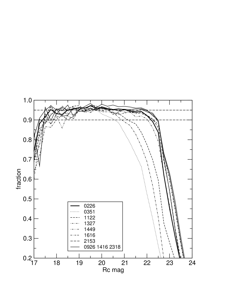
Figure 16: “Good” photometric redshift fraction vs. $R_{c}$, defined as $\sigma_{z}/(1+z)<0.15$, where $\sigma_{z}$ is the computed photometric redshift error. Each line indicates one patch. Patches 0351, 1122, and 1327 have much lower fractions at the faint end due to the poorer $V$ and $B$ data quality (see text and Figure 1). For patches 0226, 1449, 1616, and 2153, the fractions are higher than 90% for $17.5<R_{c}<22.0$. For the remaining three patches, the fractions are higher than 90% for $17.5<R_{c}<22.5$. The completeness levels increase to $R_{c}\sim 23$ mag when the criterion $\sigma_{z}/(1+z)<0.35$ is used.

All galaxies with $R_{c}<24.0$ are included in the photometric redshift catalog. The total number of galaxies is more than 1,300,000. About 168,000 objects (13% of the total) have photometric redshifts at $z<0.0$ or $z>1.5$, which are beyond the redshift range of the training set. Negative redshifts are unlikely to be physical, and because the extrapolation of the polynomial fit is very unstable, photometric redshifts $>1.5$ cannot be trusted. For these objects, we use a value of “99” to indicate this type of problematic photometric redshift in the catalog. Figure 16 presents the fraction of good photometric redshifts vs. $R_{c}$ magnitude. The definition of “good photometric redshift” is $\sigma_{z}/(1+z)<0.15$, where $\sigma_{z}$ is the computed photometric redshift error. Patches 0351, 1122, and 1327 have much poorer success rates at the faint end compared to the other patches due to poor $V$ and $B$ data quality (the limiting magnitudes for $V$ and $B$ are about 24 and 23.5, respectively, compared to the average of 24.5 and 25.0, see Figure 1). For galaxies with $17.5<R_{c}<22.0$ in patches 0226, 1449, 1616, and 2153, the fractions of good redshifts are higher than 90%. For the remaining four patches, the fractions are roughly higher than 90% for galaxies with $17.5<R_{c}<22.5$. For brighter ($R_{c}<17.5$) galaxies, the lower fractions are probably due to a lack of bright galaxies in our training set, improper star-galaxy separation due to saturated stars, saturation of bright galaxy images in one filter or more, and the lack of a sufficiently blue filter for galaxies at low redshift. For fainter galaxies, the fractions are also going down due to larger magnitude errors, especially for redder galaxies because they are even fainter in $V$ and $B$ magnitudes. According to this figure, an overall reliable completeness magnitude limit (90% to 98%) for the full catalog is $17.5<R_{c}<20.5$, while if the patches 0351, 1122, and 1327 are removed, the statistical completeness limit extends to $R_{c}\sim 22$. If we relax the photometric redshift uncertainty limit to $\sigma_{z}/(1+z)<0.35$, the completeness limit extends to $R_{c}=23$.

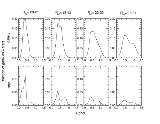
Figure 17: Redshift distributions for PPP classified galaxies and stars in different $R_{AB}$ bins. The upper four panels represent the galaxy fraction among all objects (galaxies + stars). The lower four panels show the “stars” fraction among all objects. Only for the $R_{AB}=23-24$ bin is the redshift distributions very similar between the upper and lower panels. It implies that many “stars” in this magnitude range are actually galaxies.

Because PPP star-galaxy classification begins to become less robust at $R_{c}\geq 22$ due to the low signal-to-noise ratio for faint objects (Yee, 1991), some faint galaxies are classified as stars. To test the effect and extent of misclassification, a “fake” photometric redshift catalog for point sources in each patch is also generated. If we force fit photometric redshifts to real stars, it would produce results that systematically do not have the same redshift distribution as the galaxies. Figure 17 demonstrates the photometric redshift distributions of PPP classified galaxies and stars in different $R_{AB}$ magnitude bins. The upper panels show the galaxy fraction of all objects (galaxies + stars), and the lower panels show the stellar fraction. For the $R_{AB}=20-21$, $21-22$, and $22-23$ bins, the redshift distributions for PPP classified galaxies and stars are not similar. The “fake” photometric redshifts of stars tend to be separated into two bins at $z\sim 0.4$ for the bluer disk stars, and $z\sim 0.8$ for the redder faint halo stars. The peaks for the three brighter bins do not change with magnitude, unlike those for the galaxies. But for the $R_{AB}=23-24$ bin, the shape of the redshift distributions in the upper and lower panels are very similar, which implies that a significant fraction of the “stars” are actually galaxies. Of course, we cannot rule out that high-surface brightness, concentrated galaxies (more likely to be misclassified as stars) may have a different redshift distribution compared to low-surface brightness, less concentrated galaxies.

Table 3 is an example showing the information available for each object in the photometric redshift catalog; the full photometric redshift catalog (Table 4) is available in the electronic version of the paper. Listed in the sample catalog are the following rows:

$Row(1).$—The RCS object number. The first two digits indicate the patch number, numbered 01 to 10 in the order of the patches in Table 2.1. The second two digits indicate the pointing number within a patch. The third two digits indicate the CCD chip number within the pointing. The remaining five digits represent the object number within each CCD chip.

$Rows(2)-(3).$—The R.A. in hours and Dec. in degrees (J2000).

$Rows(4)-(15).$—The total magnitudes, magnitude errors, and color errors for $z^{\prime}$, $R_{c}$, $V$, and $B$. The magnitude errors are derived from the photon noise in the optimal aperture (on total magnitude, see Yee 1991; Gladders & Yee 2004) for each object. The color errors are the sum in quadrature of the photon errors for each filter in the color aperture.

$Row(16).$—The photometric redshift.

$Row(17).$—The computed error on the photometric redshift.

Table 3: Catalog Sample

Object ID	01110800110	01110800128	01110800147	01110800158	01110800174
RA	2.435250	2.428926	2.432872	2.429133	2.432602
DEC	0.90261	0.90425	0.90534	0.90611	0.90704
$z^{\prime}$	20.81	18.70	20.04	19.27	19.43
+/- m, +/- c of $z^{\prime}$	0.05 0.04	0.01 0.01	0.03 0.02	0.02 0.01	0.01 0.01
$R_{c}$	21.00	19.36	20.58	19.98	20.04
+/- m, +/- c of $R_{c}$	0.02 0.01	0.01 0.00	0.01 0.01	0.01 0.01	0.01 0.01
$V$	21.45	20.67	21.66	21.28	21.30
+/- m, +/- c of $V$	0.04 0.02	0.01 0.01	0.03 0.03	0.03 0.02	0.02 0.02
$B$	22.23	22.06	22.79	22.58	22.67
+/- m, +/- c of $B$	0.03 0.03	0.03 0.03	0.05 0.05	0.05 0.04	0.04 0.04
Photometric Redshift	0.263	0.436	0.393	0.442	0.395
Redshift error	0.072	0.031	0.071	0.031	0.018

7 Conclusion

We present a photometric redshift catalog from the RCS data, constructed by applying an empirical polynomial fitting technique using a training set of 4924 objects with redshifts from the CNOC2 and GOODS/HDF-N samples. A 32-cell kd-tree algorithm is used to divide up our sample to improve the accuracy of the photometric redshift estimates. Our catalog includes 1.3 million galaxies in 33.6 deg² of sky (distributed over 10 patches) with redshifts less than 1.5. The rms photometric redshift scatter is $\sigma(\Delta{z})<0.06$ within the redshift range $0.2<z<0.5$, and $\sigma(\Delta{z})<0.11$ for galaxies with $0.0<z<1.5$. The computed photometric redshift errors for individual galaxies are also provided. The magnitude limit for completeness of the catalog is $17.5<R_{c}<22$ (with $\sigma_{z}/(1+z)<0.15$) if the three shallow patches (0351, 1122, and 1327) are excluded. The limit extends to $R_{c}\sim 23$ for $\sigma_{z}/(1+z)<0.35$. We also compare the redshift distribution from our catalog to the CFDF and the GOODS/HDF-N data, and the agreement between the different samples is in general very good.

We are carrying out a number of scientific studies using the photometric redshift catalog. One important example is to provide a large sample of galaxies over a large look-back time to measure the luminosity function and its evolution for field galaxies (Lin et al. 2005, in preparation). Moreover, the luminosity function for galaxies in clusters discovered by the RCS can be determined more accurately using photometric redshifts than by using two filters ($R_{c}$ and $z^{\prime}$). Furthermore, we plan to develop cluster finding algorithms using the photometric redshift catalog, creating cluster catalogs for comparison with the result from the RCS technique (Gladders & Yee, 2000, 2004). This will allow us to verify the completeness of the two-filter cluster red-sequence finding algorithm. Another topic is the search for close galaxy pairs, both in the field and in galaxy clusters, to study the evolution of the merging rate (Hsieh et al. 2005, in preparation). Such a study will provide data to test the hierarchical model of galaxy evolution. We are also using the catalog to find sub-structures (groups) in clusters, and to study the cluster population as a function of radius. Finally, the photometric redshift catalog provides accurate redshift distributions of lens galaxies and source galaxies, which are both very important for weak lensing analysis. With photometric redshift information, many weak lensing analyses, from galaxy-galaxy lensing to cosmic shear, can be improved. For example, knowing the redshifts of the lenses allows one to derive the mass-to-light ratio of galaxies as a function of galaxy luminosity (Hoekstra et al. 2005, in preparation), testing the scaling relations of bayonic and dark matter.

Figure 14: $\Delta{z}$ vs. color ($B-R_{c}$) diagram for RCS data in our training set. $\sigma(\Delta{z})$ is 0.03 for redder objects ($B-R_{c}>2$). The width of the error distribution becomes 0.043 for objects with $1.5<B-R_{c}<2$. For objects with $B-R_{c}<1.5$, this becomes larger than 0.055.

References

- Abazajian et al. (2005) Abazajian, K. et al. 2005, AJ, in press
- Benítez (2000) Benítez, N. 2000, ApJ, 536, 571
- Bentley (1979) Bentley, J. L. 1979, Commun. ACM, 19, 509
- Brodwin et al. (2003) Brodwin, M., Lilly, S. J., Porciani, C., McCracken, H. J., Le Fevre, O., Foucaud, S., Crampton, D., & Mellier, Y. 2003, astro-ph/0310038
- Bruzual & Charlot (1993) Bruzual, G., Charlot, S. 1993, ApJ, 405, 538
- Bruzual & Charlot (2003) Bruzual, G., Charlot, S. 2003, MNRAS, 344, 1000
- Budavári et al. (2000) Budavári, T., Szalay, A. S., Connolly, A. J., Csabai, I., & Dickinson, M. 2000, AJ, 120, 1588
- Capak et al. (2004) Capak, P. et al. 2004, AJ, 127, 180
- Cardelli, Clayton, & Mathis (1989) Cardelli, J. A., Clayton, G. C., & Mathis, J. S. 1989, ApJ, 345, 245
- Chen et al. (2003) Chen, H. W. et al. 2003, ApJ, 586, 745
- Coleman et al. (1980) Coleman, G. D., Wu, C. -C., & Weedman, D. W. 1980, ApJS, 43, 393
- Connolly, Csabai, & Szalay (1995) Connolly, A. J., Csabai, I., & Szalay, A. S. 1995, AJ, 110, 2655
- Cowie et al. (2004) Cowie, L. L., Barger, A. J., Hu, E. M., Capak, P., & Songaila, A. 2004, AJ, 127, 3137
- Csabai, Connolly, & Szalay (2000) Csabai, I., Connolly, A. J., & Szalay, A.S. 2000, AJ, 119, 69
- Csabai et al. (2003) Csabai, I. et al. 2003, AJ, 125, 580
- Fernández-Soto, Lanzetta, & Yahil (1999) Fernández-Soto, A., Lanzetta, K. M., & Yahil, A. 1999, ApJ, 513, 34
- Giavalisco et al. (2004) Giavalisco, M. et al. 2004, ApJ, 600, 93
- Gladders & Yee (2000) Gladders, M. D., & Yee, H. K. C. 2000, AJ, 120, 2148
- Gladders & Yee (2004) Gladders, M. D., & Yee, H. K. C. 2004, ApJS, in press; astro-ph/0411075
- Gwyn & Hartwick (1996) Gwyn, Stephen D. J., Hartwick, & F. D. A. 1996, ApJ, 468, 77
- Hogg et al. (1998) Hogg, D. W. et al. 1998, AJ, 115, 1418
- Koo (1985) Koo, D. C. 1985, AJ, 90, 418
- MacDonald et al. (2004) MacDonald et al. 2004, MNRAS, 352, 1255
- Mobasher et al. (2004) Mobasher, B. et al. 2004, ApJ, 600, 167
- O’Donnell (1994) O’Donnell, J. E. 1994, ApJ, 422, 158
- Parker, Humphreys, & Larsen (2003) Parker, J. E., Humphreys, R. M., & Larsen, J. A. 2003, AJ, 126, 1346
- Postman et al. (1996) Postman, M., Lubin, L. M., Gunn, J. E., Oke, J. B., Hoessel, J. G., Schneider, D. P., Christensen, J. A. 1996, AJ, 111, 615
- Rudnick et al. (2001) Rudnick, G. et al. 2001, AJ, 122, 2205
- Sawicki, Lin, & Yee (1997) Sawicki, M. J., Lin, H., & Yee, H. K. C. 1997, AJ, 113, 1
- Schlegel, Finkbeiner, & Davis (1998) Schlegel, D. J., Finkbeiner, D. P., & Davis, M. 1998, ApJ, 500, 525
- Wang, Bahcall, & Turner (1998) Wang, Y., Bahcall, N., & Turner, E. L. 1998, AJ, 116, 2081
- Wirth et al. (2004) Wirth, G. D. et al. 2004, AJ, 127, 3121
- Wolf et al. (2003) Wolf, C., Meisenheimer, K., Rix, H.-W., Borch, A., Dye, S., & Kleinheinrich, M. 2003, A&A, 401, 73
- Yee (1991) Yee, H. K. C. 1991, PASP, 103, 396
- Yee, Ellingson, & Carlberg (1996) Yee, H. K. C., Ellingson, E., & Carlberg, R. G. 1996, ApJS, 102, 269
- Yee et al. (2000) Yee, H. K. C. et al. 2000, ApJS, 129, 475
- Yee et al. (2002) Yee, H.K.C., Mallen-Ornelas, G., Seager, S., Gladders, M. D., Brown, T., Minniti, D., Ellison, S.L., & Mallen-Fullerton, G. 2002, Proceedings of SPIE, ed. R. Guhathakurta, Vol 4834, 150–160