Multi-epoch infrared photometric study of the star forming region G173.58+2.45

Abstract

We present a multi-epoch infrared photometric study of the intermediate-mass star forming region G173.58+2.45. Photometric observations are obtained using the near-infrared $JHKL^{\prime}M^{\prime}$ filters and narrow-band filters centered at the wavelengths of H₂ (1-0) S(1) (2.122 $\mu$m) and [FeII] (1.644 $\mu$m) lines. The H₂ image shows molecular emission from shocked gas, implying the presence of multiple star formation and associated outflow activity. We see evidence for several collimated outflows. The most extended jet is at least 0.25 pc in length and has a collimation factor of $\sim$ 10, which may be associated with a binary system within the central cluster, resolved for the first time here. This outflow is found to be episodic; probably occurring or getting enhanced during the periastron passage of the binary. We also find that the variable star in the vicinity of the outflow source, which was known as a FU Ori type star, is probably not a FU Ori object. However, it does drive a spectacular outflow and the variability is likely to be related to accretion, when large clouds of gas and dust spiral in towards the central source. Many other convincing accretion-outflow systems and YSO candidates are discovered in the field.

1 Introduction

It is now known that massive and intermediate-mass Young Stellar Objects (YSOs) drive bipolar outflows similar to their low-mass counterparts, albeit on larger scales (Shepherd and Churchwell 1996; Churchwell 1997; Cesaroni et al. 1997; Kumar, Bachiller & Davis 2002; Davis et al. 2004; Beuther, Schilke and Gueth 2004). Massive star formation occurs in clusters and is often associated with lower mass star formation. In this paper, we discuss the case of an intermediate-mass YSO G173.58+2.45, where multiple star formation is taking place within a cluster.

G173.58+2.45 (IRAS 05361+3539) is embedded in the centre of a large molecular cloud. Shepherd & Churchwell (1996) noticed that the IRAS fluxes from the embedded source meet the criteria for an Ultra Compact HII region (UCHII) (Wood & Churchwell 1989). From CO observations, they estimated a line-of-sight velocity with respect to local standard of rest, $v_{LSR}$, of -18 km s^-1, which is very close to the value of -17 km s^-1 estimated by Bronfman, Nyman & May (1996). Wouterloot et al. (1988) and Palagi et al. (1993) detected H₂O maser emission from this field. Zinchenko, Pirogov & Toriseva (1998) detected a CS($J$=2-1) core, which peaks $\sim$ 10$\arcsec$ east of the IRAS position. The kinematic distance to the source was estimated by Wouterloot & Brand (1989) to be 1.8 kpc.

This region was studied at millimeter wavelengths (in ¹²CO and ¹³CO) by Shepherd & Churchwell (1996). Their ¹²CO spectra showed high velocity line wings indicating the presence of CO outflows. They identified it as a bipolar molecular outflow candidate and estimated the mass in the outflow to be 32 M_⊙. Shepherd and Watson (2002) (SW02 hereafter) conducted detailed observations of the region at radio, mm and infrared wavelengths. CO emission line observations carried out by them detected a large scale outflow extending 3$\arcmin$.4 end-to-end, which is 1.8 pc at a distance of 1.8 kpc. At 3 mm, they also detected two continuum emission sources, which are associated with reddened infrared sources. They proposed that the outflow in this field was driven by at least two intermediate-mass YSOs.

Very few near-infrared (IR) studies of this region have been done. The H₂ image of Chakraborty et al. (2000) detected signs of nebulosity in the direction of the outflow proposed by Shepherd and Churchwell (1996). Later, more sensitive IR observations by SW02 failed to detect any signs of the jet proposed by Chakraborty et al. (2000), instead, resolved it to be a chance alignment of IR sources. However, the existing near-IR observations lack the sensitivity and spatial resolution required and hence, this study.

2 Observations

Observations were acquired with the 3.8m United Kingdom Infrared Telescope (UKIRT), Mauna Kea, Hawaii. Photometry in the $J$ and $K$ bands were obtained on 2001 Dec., 26 using UFTI (Roche et al. 2002) equipped with a Rockwell 1024$\times$1024 HgCdTe array, giving a pixel scale of 0$\arcsec$.091/pixel and a field of view of 1$\arcmin$.5$\times$1$\arcmin$.5 at the f/36 cassegrain focus of UKIRT. The region was again observed using UFTI on 2002 Oct., 22 in the $H$ and $K$ bands and in narrow-band filters at the wavelengths of the H₂ v=1-0 S(1) line (2.1218 $\mu$m) and the [FeII] $a^{4}D_{7/2}-a^{4}F_{9/2}$ line (1.6439 $\mu$m) and on 6 Nov 2002, in the $J$ band. The observations were obtained by jittering the telescope on 9 points with 20$\arcsec$ offsets from the centre resulting in a field of view of 2$\arcmin$.2$\times$2$\arcmin$.2 for the mosaics. The narrow-band H₂ and [FeII] filters have FWHM bandwidths of 0.02 $\mu$m and 0.016 $\mu$m respectively. The median seeing was $\sim$0$\arcsec$.6 on 2001 Dec. 26 and $<$ 0$\arcsec$.4 on 2002 Oct. 22 and on Nov. 6. The better seeing on the latter days enabled us to achieve excellent spatial resolution and also to detect many faint H₂ emission features. On 2003 March 19, the field was again observed in $JHK$ using UKIRT and UIST (Ramsay Howat et al. 2000), which uses a 1024$\times$1024 InSb array, at an image scale of 0$\arcsec$.12/pixel. A 9 point jitter with offsets of 30$\arcsec$ from the centre gives a field of view of 3$\arcmin$$\times$3$\arcmin$ for the UIST images. $JHK$ photometric standard stars from the list of UKIRT faint standards close to the object were always observed prior to the object in each filter. All observations were obtained under photometric sky conditions at airmass less than two. The observed magnitudes were corrected for the small difference in airmass between the object and the standard using the average extinction/airmass for Mauna Kea for each filter. Observations were again performed in the $L^{\prime}$ and $M^{\prime}$ bands using UKIRT and UIST on 2003 March 13 and Dec. 23. The observations were carried out by jittering the image on four positions on the array and taking the difference of adjacent jittered frames after flat fielding, since the background radiation is not steady at these wavelengths. On March 13, both the $L^{\prime}$ and the $M^{\prime}$ band observations were acquired using the 512$\times$512 sub-array and on Dec. 23rd, the $L^{\prime}$ band observations were carried out using the 1K$\times$1K array and $M^{\prime}$, using the 512$\times$512 sub-array. $L^{\prime}$ and $M^{\prime}$ photometric standards close to the object, from the list of Leggett et al. (2003) for the MKO-NIR system, were observed for photometric calibration. Table 1 shows the log of observations.

Table 1: Log of photometric observations

Filter	Date	Int. time	Instrument	Field of
	yyyymmdd	(sec)		view
$J$	20011226	540	UFTI	2$\arcmin$.2$\times$2$\arcmin$.2
	20021106	675	UFTI	2$\arcmin$.2$\times$2$\arcmin$.2
	20030319	90	UIST	3$\arcmin$.0$\times$3$\arcmin$.0
$H$	20021022	810	UFTI	2$\arcmin$.2$\times$2$\arcmin$.2
	20030319	270	UIST	3$\arcmin$.0$\times$3$\arcmin$.0
$K$	20011226	360	UFTI	2$\arcmin$.2$\times$2$\arcmin$.2
	20021022	1080	UFTI	2$\arcmin$.2$\times$2$\arcmin$.2
	20030319	270	UIST	3$\arcmin$.0$\times$3$\arcmin$.0
$L^{\prime}$	20030319	104	UIST∗	1$\arcmin$.3$\times$1$\arcmin$.0
	20031223	529	UIST	2$\arcmin$.7$\times$2$\arcmin$.0
$M^{\prime}$	20030319	115	UIST∗	1$\arcmin$.5$\times$1$\arcmin$.0
	20031223	553	UIST∗	1$\arcmin$.5$\times$1$\arcmin$.0
H2	20021022	900	UFTI	2$\arcmin$.2$\times$2$\arcmin$.2
$[$FeII$]$	20021022	900	UFTI	2$\arcmin$.2$\times$2$\arcmin$.2

^∗ observed using 512$\times$512 sub-array. All the rest were observed using the full 1024$\times$1024 array.

Preliminary reduction of the data was carried out using ORACDR - the pipeline data reduction facility available at UKIRT. Dark frames were obtained in each filter at the start of each set of observations. Sky flats were generated by median combining the dark- and bias-subtracted observed frames. The flat fielded individual frames were finally combined to produce mosaics using the STARLINK packages CCDPACK and KAPPA, by matching the centroids of bright stars in the overlapping fields in each pair of dithered frames. Fig. 1 shows the $JHK$ colour combined image of the field observed on 2002 Oct 22 and Nov. 6. The stars appearing red in colour are highly embedded objects and those in blue are foreground objects. Fig. 2 shows the central region of the $L^{\prime}$ image observed on 2003 Dec 23. The $M^{\prime}$ image is not shown here.

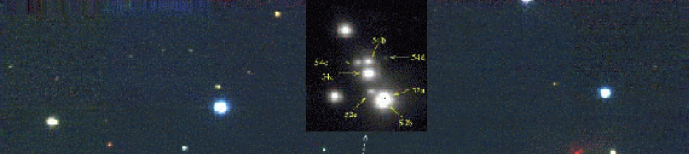
Figure 1: $JHK$ colour composite picture of the observed field constructed from the $J$ band image observed on 2002 Nov. 11 and the $H$ and $K$ band images observed on 2002 Oct. 22. Most of the objects that appear blue in colour are foreground stars and those that are yellow and red in colour are embedded in the cloud. The red sources are extremely embedded objects; many of them are YSOs with IR excess. The position of the IRAS source is marked with a ’+’. The central region is shown in the inset. The peaks of #52a and b are marked in the figure with a single contour to show the binary components. The orientation of the figure is North-up and East-left

Table 2: $L^{\prime}$ and $M^{\prime}$ photometric magnitudes. Sources outside the field of view are indicated; a dash indicates sources not detected. For #54, the $L^{\prime}$ magnitudes of the components are given only for 20031223 when the S/N was better.

No:	——- $L^{\prime}$ Band ——-		——- $M^{\prime}$ Band ——-
	20030319	20031223	20030319	20031223
14	not obs	9.92 .08	not obs
15	not obs	12.29 .15	not obs
19(a+b)	not obs	11.55 .06	not obs
25	not obs	12.35 .11	not obs
31	not obs	11.98 .09	not obs
32	not obs	12.43 .11	not obs
37	not obs	12.92 .25	not obs
38	not obs	12.31 .23	not obs
41	not obs	13.36 .35	not obs
52(a+b)	9.22 .03	9.34 .04	8.39 .06	8.49 .06
54a		10.48 .02
54b		11.98 .04
54d		12.56 .10
54(a+b+d)	10.24 .04	10.11 .03	9.50 .20	9.47 .13
58	11.27 .03	11.46 .06	–	–
59	–	12.54 .28	–	–
60	–	detected	–	–
62	–	detected	–	–
67	–	12.73 .24	–	–
68	–	12.54 .25	–	–
72	10.67 .05	10.78 .05	9.89 .14	9.76 .09
78	10.41 .10	10.66 .03	8.51 .11	8.79 .10
85	not obs	11.24 .05	not obs
90	10.24 .03	11.09 .09	9.29 .10	10.14 .20
119	not obs	11.59 .06	not obs
120	not obs	12.10 .10	not obs

The field is crowded in the $JHK$ bands. So, we estimated the magnitudes in these bands using the DAOPHOT package of IRAF, by fitting a point spread function (PSF) to the individual objects in the field. For each mosaic, the PSF is generated by fitting profiles simultaneously to several isolated stars in the field. Table 5 shows the $JHK$ magnitudes of the stars detected on all the epochs of our observations. For the $L^{\prime}$ and $M^{\prime}$ images, since fewer objects are detected, aperture photometry was done using the STARLINK display and data reduction package GAIA. Table 2 lists the $L^{\prime}$ and $M^{\prime}$ magnitudes estimated from our photometry.

SW02 carried out astrometric calibration of the field. We have, therefore, defined our coordinates to match theirs. Coordinates of the objects detected in our observations are calculated using the IRAF tasks CCMAP and CCTRAN, adopting the coordinates of some of the isolated stars from SW02 as reference. Our coordinates are West and North of the 2MASS by 0.$\arcsec$9 and 0.$\arcsec$8 respectively. In Tables 5 and 2, we have also included the identifications of SW02 and Chakraborty et al (2000), along with our new identification numbers, for ease of comparison. Many new objects are detected in our observations. Some of these objects appear to be non stellar since they shine almost equally bright in the H₂ images as in $K$. They are separately listed in Table 3. These are likely to be the molecular equivalents of ’Herbig-Haro’ (HH) objects, produced by the outflows associated with the multiple star formation activity in the region.

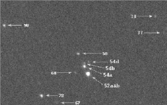
Figure 2: $L^{\prime}$ image of the central region observed on 23 Dec 2003

The narrow-band H₂ and [FeII] images were continuum subtracted using the scaled $K$ and $H$ band images respectively. For continuum subtraction, the integrated, sky subtracted counts on many isolated point sources (without any IR excess) were measured in the narrow-band filters and in the $H$ and $K$ filters using a circular aperture typically $\sim$4 times the FWHM. The ratios of the counts $K$/H₂ and $H$/[FeII] were evaluated for these stars and the average values were taken. The constant sky backgrounds were subtracted from the $H$ and $K$ band images. These images were then divided by the above ratios and were subtracted from the sky subtracted narrow-band filter images. The diffuse continuum got subtracted out well. However, stars often gave residuals due to changes in PSF between the broad- and the narrow-band observations. Continuum subtracted H₂ images (Figs. 6, 7 and 8) reveal several ’HH’ type emission features and at least six bow shocks, most of which are expected to be from shocked H₂. The continuum subtracted [FeII] image did not show any of these features except for one bow shock (B5). Therefore, it is not shown here.

3 Results and Discussion

3.1 $JHKL^{\prime}M^{\prime}$ Photometry

The coordinates of the objects detected and their magnitudes estimated for all the epochs of our observations are listed in Tables 5 and 2. The objects detected in the $L^{\prime}$ and $M^{\prime}$ band imaging are the embedded stars in Fig. 1, most of which show IR excess and a few of the brightest foreground stars. The region is studied using colour-colour and colour-magnitude diagrams.

3.1.1 Colour-colour and colour-magnitude diagrams

The near IR colour-colour and colour-magnitude diagrams are useful tools for identifying YSO candidates. Fig. 3 shows the stars plotted on the $(J-H)-(H-K)$ colour-colour diagram. Most of the data are from the UFTI observations of 2002 Oct. 22 and Nov. 6, when the seeing was best. Since the UIST mosaics cover a wider field, the stars outside the UFTI field plotted in this figure are taken from the UIST observations of 2003 Mar. 19. The continuous line shows the distribution of ($J-H$) against ($H-K$) of un-reddened main sequence stars and the dashed line, that of un-reddened giant stars, constructed from the intrinsic colours of Koornneef (1983). The lower end of the curve marks the early type stars and the upper end, the late type stars. The diagonal parallel lines are the reddening vectors up to A_V=30, at the maxima of the main-sequence and the giant stars’ colours and at the minimum of the main sequence colours. This is the direction in which reddening moves the stars in the colour-colour diagrams. We adopted a reddening law with R_V=(A_V/E($B-V$))=5, which is typical for dense clouds (Cardelli, Clayton & Mathis 1989). This gives values of extinction varying from A_J=9.82 to A${}_{L^{\prime}}$=1.66 for $J$ to $L^{\prime}$ at A_V=30. The stars in the reddening band, the region between the parallel lines, are main-sequence and giant stars at different reddening within the cloud and along the line of sight. The region below the lower line is occupied by YSOs (Lada & Adams 1992), where CTTS, WTTS, HAeBe stars and luminous YSOs occupy different regimes. The excellent spatial resolution has enabled us to resolve the multiplicity of many objects, which were perceived as singles in the previous investigations. The colours of these objects measured as singles and also of the resolved component stars measured individually are plotted in the figure.

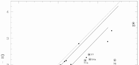
Figure 3: ($J-H$) - ($H-K$) colour-colour diagram of the field derived from our observations. The continuous line shows the locus of the un-reddened main sequence stars and the dashed line, that of giant stars. The straight lines show the reddening vectors up to A_V=30.

In Fig. 4, we have plotted the $K$ magnitudes of the objects against their ($H-K$) colours. The continuous line is the location of the un-reddened main sequence stars from Koornneef (1983) at a distance of 1.8 kpc. The location of the different spectral types are marked on this line. The dotted lines show the reddening vectors up to A_V=30. As in Fig. 3, the locations of the individual components of multiples and that of the components put together are separately shown. For reddened main sequence stars, extrapolation of the stars back along the reddening vector to the main-sequence line should give their spectral types. However, many of the reddened stars, especially the YSOs, will have infrared excess arising from circumstellar matter, which makes them brighter towards longer wavelengths and thereby, moves them up in the colour-magnitude diagram. So, great caution has to be taken when drawing conclusions about spectral types from the colour-magnitude diagram. For objects with infrared excess, it should be treated only as an upper limit to the spectral type.

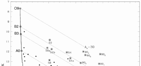
Figure 4: $K-(H-K)$ colour magnitude diagram. The continuous line shows the locus of main sequence stars at a distance of 1.8 kpc. The straight lines show the reddening vectors up to A_V=30. Stars showing IR excess are circled.

Similarly, an ($H-K$) - ($K-L^{\prime}$) colour-colour diagram (Fig. 5) is constructed using the infrared colours for main sequence and giant stars given by Bessell & Brett (1998). Most of the stars detected in the $L^{\prime}$ band are those with IR excess in the $K$ band and a few bright foreground stars. The YSO candidates are enclosed in circles and are labelled in the figure. These objects, which show IR excess in Figs. 3 and 5, are discussed in section 3.3.

3.2 The narrow-band H₂ and [FeII] imaging

Narrow band imaging at the wavelength of the H₂ (1-0) S(1) line at 2.122 $\mu$m is very useful for detecting shock excited emission from molecular hydrogen and, thereby, the ongoing star formation and outflow activity in embedded regions. Fig. 6 shows the continuum-subtracted H₂ image observed using UFTI. Many of the emission features detected are labelled in the figure and their coordinates and integrated fluxes are listed in Table 3. Arrows are drawn in the direction of three well aligned sets of emission knots; one set is probably produced by the bright source (IRS1) located near the centre of the field. Many of the H₂ emission features are seen to be associated with reddened objects in the field, which are described below. Some features, which are enclosed in circles, are not positively traced back to any specific object in the field. These features could be from some of the objects described below or from embedded objects, which are not detected at the current depth of integration.

We used an integration time of 900 seconds in both the filters, which, in [FeII], gave a 3$\sigma$ sensitivity of $\sim$ 2 $\times$ 10^-20 W m^-2 pix^-1. Interstellar extinction at 1.644 $\mu$m will be higher than at 2.122 $\mu$m (A_[FeII]/A${}_{H{{}_{2}}}$ $\sim$1.5). Also, for weak shocks, the line flux at [FeII] 1.644 $\mu$m is typically lower than that at H₂ 2.122 $\mu$m (Smith 1995). So, for most of the faint H₂ features, their non-detection in [FeII] can be attributed to the extinction and to the shocks being relatively weak. The lack of [FeII] emission may also be a sign of weak molecular shocks being more common than strong atomic shocks. H₂ and [FeII] line emission are often observed in jets and bow shocks from low mass young stars (e.g. Reipurth et al. 2000; Davis et al. 2003), although the emission usually derives from different regions in each outflow. The H₂ is usually excited in the oblique wings of bow shocks, where low shock velocities, low ion fractions and modest magnetic field strengths generate bright molecular line emission. The [FeII] is instead excited in the compact apices of bow shocks, or in jet Mach disks, where shock velocities are much higher and excitation conditions are more extreme.

So, although the sensitivity of our [FeII] observations is limited, and extinction will play a role, it is nevertheless interesting that these extreme excitation conditions (the Fe⁺ ionization fraction is predicted to peak at temperatures of $\sim$14,000 K [Hamann 1994], and the critical density for collisional excitation of the 1.644 $\mu$m [FeII] line is $3\times 10^{4}$ cm^-3) do not seem to be prevalent across the field observed except for B5, which is the only H₂ features showing [FeII] emission.

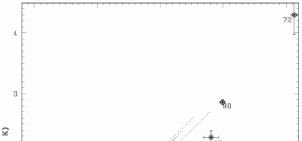
Figure 5: $(H-K)-(K-L^{\prime})$ colour-colour diagram. The continuous line show the locus of main sequence stars and the broken line, that of giants. The dotted lines show the reddening vectors up to A_V=30.

3.3 Discussion of individual sources

3.3.1 Outflow sources in the central cluster

At the current spatial resolution, the central source IRS1 (#52) itself is resolved to have three components, with 2 stars of similar brightness (#52a and b) at a separation of 0.40$\arcsec$$\pm$ 0.01, with the apparent line of centres oriented 153.5${}^{\circ}\pm$ 1^∘ east of north and a much fainter component (#52c) at a separation of 1.35$\arcsec$$\pm$ 0.01 from the apparent line of centres of the binary, at an angle 54.7${}^{\circ}\pm$ 1^∘ east of north. Contrary to what was noticed by SW02 for IRS1, #52a and b show IR excess in the $JHK$ colour-colour diagram (Fig. 3). Both these objects are well detected and are the brightest ones in the $L^{\prime}$ and $M^{\prime}$ bands. #52c appears in the main sequence reddening band in the $JHK$ colour-colour diagram. It is located at the position of a reddened O type star. Nevertheless, this star is the faintest of the three, being fainter than the binary components by 3.4 magnitudes in $K$. So, if this is a reddened O star, it would be brighter in the $L^{\prime}$ and the $M^{\prime}$ bands and would have been detected in our $L^{\prime}$ images. The fact that it is not detected at wavelengths higher than $K$ implies that #52c is not a reddened O star, but a star of much later type, with some amount of IR excess, which moves it to the region of reddened O stars in Fig. 3. The position of the star in the colour-magnitude diagram (Fig. 4) justifies this. We conclude that #52c is a reddened late type star with IR excess; the upper limit of its spectral type is $\sim$F5. The combined magnitude of the sources in #52 does not show any variability.

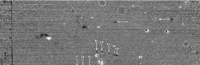
Figure 6: The continuum subtracted H₂ image of the central region. The image is shown as negative to enhance the H₂ emission features. The ’Herbig-Haro’ type features and bow shocks detected are labelled. Arrows are drawn along the aligned H₂ knots. The well aligned H₂ features strongly suggest collimated jets.

The feature towards the north-east of #52 (source #19 of Chakraborty et al. 2002 and SW02) is not a jet, as previously noticed by SW02. In our $JHK$ images, it is resolved into four stars, #54a-d, ranging from 12.67 mag. to 17.72 mag. in the $K$ band. All four stars show IR excess. #54c, the star with the least excess of the four is not detected in $L^{\prime}$ and $M^{\prime}$, whereas #54d, the faintest of the four is detected only in the $K$ and $L^{\prime}$ bands and is heavily reddened. #54a-c exhibit photometric variability. We find evidence of at least one (and possibly two) YSOs associated with sources #52 and #54. A well collimated outflow extends in the north-east(NE) - south-west(SW) direction, which can be traced along the H₂ emission features labelled B1-B3 located NE and A1-A2 located SW of the central cluster in Fig. 6. All these features appear well detected in the $K$ and H₂ images. The brightest of the three in the NE direction, B2, is marginally detected in the $H$ and $J$ bands, which are likely to be due to H₂ emission lines in these bands. B2 is much brighter in our $K$ band and H₂ images and would, if plotted in a $(J-H)-(H-K)$ colour-colour diagram, appear in the lower right region of the plot, as predicted by molecular shock models (Smith 1995). The direction of the bow shocks B1-B3 show that these are driven by one or more of the objects in the central region enclosed in the box in Fig. 1, most likely from the binary #52a and b. We do not see any bow shocks in the opposite direction, although we see sets of H₂ knots extending SW from source #52, which we label A1 and A2, both resolved into two components each, named A1_1, A1_2 and A2_1,A2_2 respectively in Fig. 6. These are probably produced by the counter jet. B1, B2 and B3 and A1 and A2 are certainly well aligned with #52 and are oriented at an angle 26^∘ east of north. An arrow is drawn connecting them in Fig. 6. The jet appears very well collimated with a collimation factor of at least 10, measured between B2 and source #52. Note, however, that the direction of this jet is different from the direction of the main outflow observed in the CO line emission by SW02, which was at 79^∘. The CO maps have poorer resolution and so, may not be resolving individual outflows.

Two other sets of H₂ emission features C1 - C4 and C5 - C7 are evident in Fig. 6. These are aligned in the opposite directions of the central cluster, though they are clearly not the two lobes of the same outflow. Two arrows are drawn in the figure in the directions of these features. They are likely to be caused by the outflows from more than one source in #54 and in the central cluster. Also obvious are the features marked A3 and A4 in the figure; A3 is resolved into two four components labelled A3_1,A3_2, A3_3,A3_4 and A4 is resolved into two, labelled A4_1,A4_2. The positions and H₂ fluxes of all these features are listed in Table 3. Together, these observations prove that the central region of G173.58+2.45 is indeed active in star formation and that there are multiple objects driving outflows.

3.3.2 Is the binary #52a,b responsible for the outflow causing the bow-shocks B1 - B3 ?

If the components of the visual binary #52a,b are dynamically related, assuming the observed separation of the binary to be a lower estimate of the major axis of the orbit and adopting the masses of the components to be $\sim$7.6 M$\odot$ each for the two stars for their upper limit of spectral types, B3, using Kepler’s equation, we get a lower estimate of 1700 years for the period of the binary orbit. Since the major axis could be longer and the binary period is more sensitive to the semi-major axis than the masses of the components, this period is only a lower estimate. B1 and A1_1, A1_2 are at an average distance of 10$\arcsec$ and B2 and A2_1, A2_2 are at an average distance of 24$\arcsec$ from #52. Assuming a jet velocity of $\sim$100 km s^-1 (Reipurth & Bally 2001) in the sky plane, we get a dynamical time of 850 years for B1 and A1_1, A1_2, if they originate from #52. The age will be higher than this, depending on the angle of inclination. Similarly, B2 and A2_1, A2_2 will have a dynamic age of $\sim$2075 years or more, for an outflow velocity of $\sim$100 km s^-1, if they originate from #52. This similarity of the orbital period with the dynamical age of the outflow estimated from the H₂ knots suggests that they might be related. All these features are probably associated with the binary #52a and b. Both the components must be having accretion disks around them. The mass accretion and outflow must be episodic, probably occurring or getting enhanced during the periastron passage of the binary stars, and thereby giving rise to the features B1, B2, B3 and A1s and A2s. The H₂ image (Fig. 6) also shows features A3_1-4 and A4_1-2, and the two features further south, which are enclosed in boxes. It is possible that these features are related to A1 and A2 and might be caused by the precession of the jet. But we cannot rule out the possibility that A3s and A4s are driven by other sources in the region, like those in #54. There are many other fainter H₂ emission features enclosed in circles in Fig. 6. Specially noticeable among those are the ones towards the left half, running almost horizontally. These features are roughly in the direction of the CO outflow (Fig. 5 of SW02).

Table 3: Observed fluxes of ’Herbig-Haro’ type objects at the wavelength of 2.122 $\mu$m H₂(1-0)S(1) line in the field

Feature	Coordinates	2.122 $\mu$m line flux
	RA,Dec(J2000)	($\times$ 10-19 W/m2)
B1	5:39:27.31 35:41:01.7	16.5
B2	5:39:27.84 35:41:15.9	75
B3	5:39:28.06 35:41:20.3	38
B4	5:39:26.45 35:41:18.5	18
B5	5:39:25.38 35:40:53.0	68
B6	5:39:24.47 35:40:32.2	9.6
A1_1	5:39:26.65 35:40:45.0	9.2
A1_2	5:39:26.61 35:40:42.8	17.8
A2_1	5:39:26.21 35:40:32.9	17.8
A2_2	5:39:26.20 35:40:31.4	13
A3_1	5:39:25.78 35:40:35.8	8.8
A3_2	5:39:25.66 35:40:34.4	12.6
A3_3	5:39:25.75 35:40:34.1	11.7
A3_4	5:39:25.98 35:40:35.3	10.7
A4_1	5:39:26.12 35:40:43.8	30.4
A4_2	5:39:26.01 35:40:42.2	29
C1	5:39:26.42 35:40:59.8	19.7
C2	5:39:26.52 35:41:00.0	15.3
C3	5:39:26.75 35:41:00.9	10.7
C4	5:39:27.06 35:41:01.7	11.5
C5	5:39:27.59 35:40:53.4	7.3
C6	5:39:27.89 35:40:53.8	13.2
C7	5:39:28.14 35:40:53.1	19
D	5:39:28.91 35:40:44.5	19
#65’s bow shock	5:39:27.71 35:40:29.0	2051
#76	5:39:28.57 35:40:35.9	1992
#76+neb		3563
E	5:39:24.01 35:41:19.5	29.5

Integrated fluxes: ¹ in a 20 pixel radius window enclosing the emission nebulosity near #65, ² in a 10 pixel radius window enclosing #76abc, ³ in a 33 pixel radius window enclosing #76abc and the emission bridge between #76 and #78

3.3.3 #37 and #19

#37 is a deeply embedded source. The $K$ magnitude is $\sim$ 16.5 and is variable. Our $K$ image shows a faint ’comet’ shaped nebulosity associated with it, which disappears in the continuum-subtracted H₂ image. The source is faint, but detected in the $L^{\prime}$ band.

Source #19 is a visual binary, both the components of which (#19a and b, separated by 0$\arcsec$.96) appear reddened. There is a nebulosity around them in the $K$ band, which disappears in the continuum-subtracted H₂ image. The component stars are not detected in the $H$ band, but a faint nebulosity is present. The source is bright in the $L^{\prime}$ band, most of the contribution appearing to come from #19a.

3.3.4 Outflow source #65

#65 is detected only in the $K$ band and is a deeply embedded. There is a strong ’cap’ like emission in H₂ towards the north-east of the source at a separation of $\sim 1\arcsec$. This feature appears split into two and the continuum subtracted H₂ image shows that it is mostly emission in H₂. It is very likely that #65 drives an outflow, which is highly inclined with respect to the sky plane. The ’cap like’ feature in H₂ is probably the bow shock of the blue-shifted lobe of the outflow, inclined in our direction. Extinction probably obscures our view of the red-shifted lobe. There are two other extremely red sources, #60 and #62, situated NW of #65, which are well detected in $K$ and are brighter than #65. The sources appear deeply embedded and are marginally detected in the $L^{\prime}$ band. There is faint H₂ emission very close to #62 and the star exhibits variability in $K$.

3.3.5 The extremely red object, #72

#72 is one of the reddest objects in in the region. This source was detected in all our $K$ band images. It was not detected in the $J$ band and was only weakly detected in $H$ on 2002, Oct. 22, when the seeing was $<$0.4 and the integration was deep. It is bright in the $L^{\prime}$ and $M^{\prime}$ bands and it stands out in both the $(H-K)-K$ colour-magnitude diagram (Fig. 4) and in the $(H-K)-(K-L^{\prime})$ colour-colour diagram (Fig. 5). The locations of the object in these diagrams give the appearance of a late O or early B star with very high extinction. Since the object was not detected in the $H$ band on 2003 March 19, we have used the $L^{\prime}$ magnitude of 2003, March 19 along with the $HK$ magnitudes of 2002 Oct. 22 to place this star on the $(H-K)-(K-L^{\prime})$ colour-colour diagram. So, the location of the star close to the reddening band in Fig. 5 cannot be considered as due to a lack of IR excess. The $H$ band magnitude has a large uncertainty of 0.32 mag and the the object exhibited variability in $K$ during the three epochs of our observations. Note that $(H-K)$ colour also will not be free from IR excess. This object is very likely to be a YSO with a considerable amount of circumstellar matter; indeed, the $K$ band image shows a well defined ’comet’ shaped nebula associated with it. We detect no H₂ emission from this nebula, which is probably dominated by reflection and/or thermal emission by dust. The source is as close to the IRAS positions as #52.

3.3.6 Outflows from the embedded binary, #78

This is a set of interesting objects, with #76 located south-west of #78. The region is shown in detail in Fig. 7. Both sources are resolved into three components each, with #78 showing a tighter association. The components of #78 are named #78a,b and c based on their decreasing brightness in the $K$ band. #78a,b appear to be point sources, but #78c is slightly extended and may be part of an outflow. The components of #76 are labelled #76a,b and c. #76c disappears in the continuum subtracted H₂ image (Fig. 7) while #76a and b appear like point sources. There is a bridge of nebulosity connecting #76 and #78, which is mostly H₂ emission. The projected separation between #76 and #78 is 3$\arcsec$, which is 0.026 pc (5400 AU) at a distance of 1.8 kpc.

Though both #76 and #78 are of comparable brightness in $K$, their $JHK$ colours (Fig. 3) show that #76 is more reddened than #78. There is no trace of #76 in the $L^{\prime}$ and $M^{\prime}$ images. #78 is well detected in both $L^{\prime}$ and $M^{\prime}$ bands and the IR colours place it in the region of the colour-colour diagrams (Figs. 3, 5) occupied by YSOs. So, #78 is probably a set of two young outflow sources, which are responsible for the H₂ emission in Fig. 7 (around #76 and between #76 and #78). Note that there is a faint emission (D) in the counter-flow

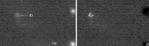
Figure 7: The left portion of the figure shows the observed H₂ image and the right portion shows the continuum subtracted H₂ image of #76, #78 and the emission in between. The contours are at flux levels 3.0, 1.5, 0.8, 0.5 and 0.25 $\times$10^-19 Wm^-2pix^-1 (1 pixel of UFTI=0.00825 arcsec²).

direction. Both #76 and #78 appeared to be continuously fading in the $JHK$ bands within the period of our observations, with #76 fading faster than #78. #78 exhibited fading in the $L^{\prime}M^{\prime}$ bands too. The coordinated fading in the $JHK$ bands implies that #78 and #76 are probably related and the emission from #76 and and the bridge between #76 and #78 depend on #78 for the source of energy. However, Table 5 shows that on 2000 Dec. 26, #76 was brighter than #78 in the $J$ and $K$ bands. This scenario is possible if the emission from #76 is mostly contributed by line emission from shocked H₂. (The fact that #76c disappears in the H₂ image upon continuum subtraction shows that there is also some amount of reflection and/or emission from dust contributing to #76). It is also likely that #76-#78 direction is inclined very much with respect to the sky plane so that #76 suffers from much less extinction compared to #78 in an inhomogeneous medium. The much fainter H₂ emission in the opposite direction strengthens this argument. Alternatively, there is a possibility that #78 and #76 are two different sets of objects, the medium around #76 emits mostly in H₂ and that the coordinated variability that we see is merely a coincidence. But, considering the fact that #76 is not detected in the $L^{\prime}$and $M^{\prime}$ bands even though it is nearly as bright as #78 in the $JHK$ bands and that it lies in the middle-right portion of the $(J-H)-(H-K)$ colour-colour diagram, close to the region occupied by reddened shocks (Smith 1995), it is more likely to be composed of reddened bow shocks of the outflow from #78.

From their spatial locations and $HKL^{\prime}M^{\prime}$ colours, it seems likely that #72 and #78 contribute significantly to the IRAS fluxes. These two sources could be two of the prominent candidates for driving the CO outflow seen in the field by SW02.

3.3.7 The variable outflow source, #90

In Fig. 8, we focus on the region around #90. Chakraborty et al. (2000) first detected the variability of source #90 (their #12). They proposed that this might be due to FU Orionis type behavior. Later NIR observations by SW02 confirmed the variable nature of this star. Our multi-epoch NIR observations also confirm the variability of this star. All the available $JHK$ magnitudes of this object are compiled in Table 4, which shows the variability of the source at these wavelengths. The $J$ and $H$ band filters used by all the investigators are similar. Chakraborty et al. (2000) observed using a $K^{\prime}$ filter and SW02 and 2MASS used $K_{s}$ filter which both have their central wavelengths shorter than 2.2 $\mu$m of the $K$ filter used by us. An inspection of the magnitudes estimated for some of the bright non-variable stars in the field shows that our estimates agree with that of 2MASS within 0.04 mag in all bands, with that of Chakraborty et al. within 0.1 magnitudes in the $J$ band and within $\sim$0.12 mag in $H$ and $K$ and with SW02 within 0.05 mag in the $J$ band and $\sim$0.1 mag in the $H$ and $K$ bands. The differences between the photometric systems is less than these and are ignored. The photometric variability that we see on this source is higher than these differences and the photoemtric errors. It can be seen from Table 2 that the object shows co-ordinated variability in the $L^{\prime}$ and $M^{\prime}$ bands also over the two epochs of our observations. In Fig. 9, we have plotted the observed $JHK$ magnitudes of this star against the Julian dates. The calendar days are also shown in this diagram. Magnitudes quoted by Chakraborty et al. (2000), SW02 and from 2MASS are included along with ours. Together, these give 6 epochs of data in $K$, from 1997 October to 2003 March. The object is detected in $J$ only on those epochs when it is brightest in $K$. It is too early to say if there is any periodicity in its variability. The nature of the variability is unlike that of a typical FU Ori type, which show longer time scales, of the order of tens of years. (A review of the properties of FU Ori objects can be seen in Hartmann & Kenyon 1996).

This star has large $JHK$ colours and large IR excess, as can be seen in Figs. 3 and 5. It also shows an extended, well collimated, nebulosity, which appears to originate from the star. The nebulosity is not seen in the $H$ band and is seen well in the $K$ band and H₂. The continuum subtracted H₂ image shows that the emission in the nebulosity is mostly at 2.122 $\mu$m. This implies that the emission is mostly from shocked molecular Hydrogen. The large infrared colours and the nature of the nebulosity tells that this object is a YSO, with an accretion disk and an outflow.

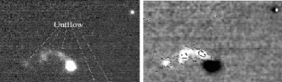
Figure 8: The left portion of the figure shows the observed H₂ image of star $\#$90 and its outflow. The right portion shows the continuum subtracted, smoothed, H₂ image on which line intensities are plotted as contours. The contours are at 2.0 and 0.5 $\times$ 10^-20 Wm^-2pix^-1 respectively.

Table 4: Observed magnitudes of Source #90

Cal. date	JD	$J$	$H$	$K$
	2400000+
97Oct181	50739.5	17.99(.04)	14.70(.01)	12.35(.01)
98Feb032	50847.5	17.15(.18)	14.29(.04)	12.01(.01)
00Jan103	51553.5		15.32(.07)	13.14(.07)
01Dec254	52270.01			14.01(.02)
02Oct224	52570.06		15.16(.02)	12.26(.01)
02Nov064	52584.98	18.73(.04)
03Mar194	52717.8		16.09(.03)	13.23(.02)

¹SW02, ²2MASS, ³Chakraborty et al. (2000), ⁴present work

Left portion of Fig. 8 shows the observed H₂ image of #90. The brighter part of the outflow points towards the NE and has a twisted appearance; careful inspection shows that there is also some H₂ emission in the SW direction of this star, though this is much fainter than the NE component. We are probably seeing a bipolar outflow, which is somewhat inclined with respect to the line-of-sight. The differential extinction due to the inclination and the inhomogeneity of the surrounding medium must be contributing to the large difference in brightness between the NE and SW outflows. The continuum subtracted H₂ image of the region is Gaussian smoothed with

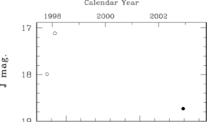
Figure 9: Variation in the $JHK$ magnitudes of star #90. The open circles show the previous observations and the filled circles show our observations.

a Gaussian of 3 pix FWHM to enhance the contrast of the faint H₂ emission, especially the SW lobe, in the presence of the background noise. The right half of Fig. 8 shows the continuum subtracted, smoothed H₂ image on which line fluxes are plotted as contours. It is interesting to note that the direction of the brighter lobe of the outflow observed in the H₂ image matches roughly with one of the blue-shifted emission lobes (in the NE direction) in the CO line emission map of SW02. The twisted nature of the NE outflow suggests that there is probably a precession of the object or jet, which results in time dependent variations in the direction of the outflow. Alternatively, we are looking at a partially shocked shell at the edges of a parabolic outflow. High resolution spectroscopy of the outflow at 2.122 $\mu$m would shed further light on the geometry of this system.

The $JHK$ light curves (Fig. 9) show that the flux variations are coordinated in all three bands. The first pair of points (97Oct18, 98Feb03) show the variations increasing towards shorter wavelengths. This type of colour dependence of the variability in the $JHK$ bands can be caused by obscuration by dust clouds passing in front of the star, which spiral in towards the star when accreted. However, if the variations are purely due to variable extinction, then we should see a shift in the position of the star parallel to the reddening vectors in the $(H-K)-K$ colour-magnitude diagram in Fig. 4 when we plot the data from the different epochs. We have plotted all the available simultaneous $HK$ observations of the source from Table 4 in the figure. 90₁ and 90₂ show the location of our observations; 90₃ shows the observation of Chakraborty et al. (2000); 90₄, the 2MASS observations and 90₅, that of SW02. We can see from the figure that, though 90₁, 90₄ and 90₅ are located close to a reddening line, 90₂ and 90₃ deviate very much. Accordingly, the pairs (98Feb03, 00Jan10) and (02Oct22, 03Mar19) do not show any colour dependence in the $H$ and $K$ magnitude variations in Fig. 9, though though they vary simultaneously. Thus, the shift in the location of the object in the colour-magnitude diagram is not caused by reddening alone. Instead, the variability is likely to be due to a combination of mechanisms, like changes in the accretion luminosity due to variable accretion and variable reddening caused by large clumps of dusty material crossing the line of sight when they spiral in towards the central star. At this stage, we cannot say if there is any binarity involved. The large reddening and the observed bipolar H₂ emission imply that the object is in an actively accreting phase. In these type of objects, it is natural that the accretion luminosity may be comparable to the stellar luminosity (Herbst & Shevchenko 1999). In the $(J-H)-(H-K)$ colour-colour diagram, the object is located towards the region occupied by luminous YSOs (Lada & Adams 1992). Observations at longer wavelengths are required for a proper estimate of the luminosity of this object. More observations of this star are being planned.

3.4 Observations at longer wavelengths

The region was imaged in the IRAS mission. The IRAS positions (IRAS 05361+3539, $\alpha$=05:39:27.7, $\delta$=+35:40:43, J2000) are east of #52 by 10$\arcsec$.5 and south by 10$\arcsec$.3. Source #72 (with the cometary nebula) is the object closest to the IRAS positions; #72 also has strong colours in the $JHKL^{\prime}M^{\prime}$ bands. It is well detected only in $K$ or above; in $H$, it is only marginally detected. The IRAS position is marked by a ’+’ sign in Fig. 1. The error ellipse of the IRAS positions is (32, 7, 86), ie., the source can be said to be located within an ellipse of semi-major axis 32$\arcsec$ and semi-minor axis 7$\arcsec$ with the semi-major axis inclined at an angle of 86^o E of North, with 95% confidence. Looking at the $L^{\prime}$ and $M^{\prime}$ images observed by us and their location with respect to the IRAS coordinates, it is highly likely that the flux measured by IRAS is the combined emission by a number of stars, particularly #72, #78, #52 and #54.

SW02 detected two mm wavelength continuum emission sources, MM1 and MM2, using interferometric observations at 2.7 mm within a field of 5$\arcmin$.3 $\times$ 3$\arcmin$, which were interpreted as due to thermal dust emission associated with embedded protostars. The location of MM1 ($\alpha$=05:39:28.67, $\delta$=+35:40:37.8) matches closely with #78 in our near IR images, located between #78 and #76. From the fact that #76 is not detected in the $L^{\prime}$ and $M^{\prime}$ bands, #78 is the most likely counterpart of MM1. The location of MM2 ($\alpha$=05:39:27.08, $\delta$=+35:40:56.1) matches well with #54, being located between #54 a,b & d. All four objects in #54 come within their beam. We cannot say for sure if there is no contribution to MM2 from #52. Assuming optically thin dust emission, they determined a mass of 12 M_⊙ for the gas and dust associated with MM1 and 7M_⊙ for MM2. This is consistent with the larger $JHK$ colours observed for #78 compared to the colours of the components of #54. Also the larger amount of nebulosity and the indications of outflow from H₂ emission implies that #78 is younger than #54 and has more gas and dust associated with it.

Methyl Cyanide (CH₃CN) emission is observed from warm, dense molecular cloud cores, which are believed to be heated by embedded massive protostars during the pre-UCHII phase of massive star formation. The 220 GHz CH₃CN survey of Pankonin et al. (2001) failed to detect any emission from the vicinity of IRAS 05361+3539, showing that either the emission is too faint or the IRAS source or the objects near it have evolved past the very early stages. In a CH₃OH maser survey conducted by Blaszkiewicz & Kus (2004), 12.2 GHz maser emission was found from this region with a peak flux density of 12.5 Jy at a position slightly different from the position of the 6.7 GHz emission observed by Menten (1991). They did not detect any 6.7 GHz emission, though Menten (1991) detected a weak 6.7 GHz maser source (peak 5Jy) in this region. The central coordinates of Blaszkiewicz & Kus (2004) match closely with the centre of our IR images, whereas that given by Menten (1991) are south of this position by $\sim$ 10$\arcmin$ and may not coincide with that of Blaszkiewicz & Kus (2004). Note that Menten’s observations used a beam size of 5$\arcmin$ whereas the observations by Blaszkiewicz & Kus have a beam size of 3$\arcmin$ at 12.2 GHz and 5$\arcmin$.5 at 6.7 GHz. Also the line-of-sight radial velocities of both detections are different. 12.2 GHz maser emission is associated with class II 6.7 GHz masers, which are usually observed towards UCHIIs, whereas class I 6.7 GHz masers are associated with outflow shocks (Blaszkiewicz & Kus 2004, Plambeck & Menten 1990). This implies that there is a UCHII region present towards the centre of the field, though we do not identify this object specifically in our IR images.

4 Conclusions

Detailed multi-epoch photometry of the intermediate-mass YSO, G173.58+2.45, and its surrounding cluster is performed at high spatial resolution in the infrared $JHKL^{\prime}M^{\prime}$ photometric bands and at the wavelengths of 2.122 $\mu$m H₂(1-0) S(1) and 1.644 $\mu$m [FeII] using narrow band filters. Through the infrared colours and the presence of bow shocks and other outflow features seen in the H₂ images, we identify many of the outflow sources. It is shown that the outflow seen in this region in low-resolution CO maps is due to multiple collimated outflows.

The source detected by IRAS (IRAS 05361+3539) is probably the combined emission from a number of YSOs near the central part of the field; the prominent ones appear to be the sources #72, #78ab, #52ab and #54abd.

From the apparent separation of the binary components #52ab and an assumption about their masses, an estimate of the lower limit of the orbital period is made. If we assume a typical flow velocity of 100 km s^-1, there is a reasonably good agreement between the binary period and the difference in the dynamical times of the individual sets of aligned H₂ emission features. This shows that the mass accretion and the associated outflow are episodic and must be occurring or getting enhanced during the periastron passage of the binary system. However, this source doesn’t appear to be the the main contributer to the outflow discovered in the CO emission lines.

Source #90 is associated with a well defined outflow, both the lobes of which are detected in H₂ emission. The presence of these outflow lobes indicate that there is ongoing accretion. This object shows large photometric variability. We do not have a sufficient number of observations of this star to look for periodicity. However, the very twisted appearance of the outflow may be an indication of the precession of the object or the jet or of the presence of a partially shocked shell at the edges of a parabolic outflow. The large photometric variability could be due to varying amount of accretion. An obscuration mechanism alone is not sufficient to explain the nature of the photometric variability. Instead, the variability could be due to a combination of phenomena, like variations in the accretion luminosity and variable obscuration from accreting circumstellar matter. From the present data, we cannot establish whether this object has a companion. The object definitely needs follow-up photometric observations at shorter time intervals and at high angular resolution for a more complete understanding.

Two objects (#72 and #90) exhibit IR colours similar to that of massive YSOs. Observations at longer wavelengths at high spatial resolution are required to estimate their luminosities.

Several other YSOs are detected in the field from the H₂ images and the IR colours. Many of these YSOs show photometric variability. The YSO candidates detected appear to be in different stages of their protostellar evolution. These observations show that this is a region very active in star formation and that the star formation is not coeval.

Appendix A $JHK$ Photometric observations

Table 5: $JHK$ Photometric magnitudes of sources within 3$\arcmin$$\times$3$\arcmin$ of IRS1. The error estimates are shown against the estimated magnitudes.

No:	SW02	RA	Dec	—————- $J$ Band —————-			——– $H$ Band ——–		—————- $K$ Band —————-
	ID	J2000	J2000	20011226	20021106	20030319	20021022	20030319	20011226	20021022	20030319
1		5:39:20.73	35:41:27.8					16.33 .06			15.50 .08
2		5:39:20.85	35:41:04.3			17.39 .14		16.87 .07			16.32 .12
3	26	5:39:21.60	35:40:21.9					16.15 .06			15.41 .08
4		5:39:21.98	35:41:13.4				19.49 .15			18.09 .05
5		5:39:22.09	35:41:47.3							17.68 .05
6	16	5:39:22.36	35:40:57.4		16.70 .05	17.00 .12	16.22 .03	16.42 .06		15.84 .02	16.05 .10
7	24	5:39:22.39	35:40:34.8		16.52 .04	16.57 .10	15.30 .02	15.28 .02		14.60 .01	14.60 .02
8		5:39:22.54	35:41:10.7		17.97 .12		17.52 .06			17.13 .03
9		5:39:22.56	35:40:06.3							18.67 .12
10		5:39:22.60	35:40:56.6				18.55 .05			16.90 .05	16.95 .12
11		5:39:22.68	35:40:20.8				19.72 .20			18.76 .11
12	1	5:39:22.82	35:41:28.6		16.36 .05	16.07 .05	15.12 .02	15.13 .02		14.47 .01	14.46 .04
13		5:39:22.92	35:39:53.8			17.67 .15					16.86 .12
14	2	5:39:22.92	35:40:23.9			10.37 .02		10.11 .02			10.01 .01
15	3	5:39:22.93	35:41:41.8		12.89 .00	12.85 .02	12.63 .01	12.61 .02		12.52 .01	12.52 .02
16a		5:39:22.99	35:41:27.9				19.08 .10			17.59 .04
16b		5:39:23.01	35:41:27.4							17.91 .05
16		16(a+b)+nebula					17.98 .10			16.46 .15	17.03 .11
17		5:39:23.09	35:40:04.0							19.60 .25
18	17	5:39:23.11	35:41:18.3	16.67 .07	16.50 .04	16.64 .05	15.88 .04	15.96 .03	15.64 .01	15.50 .01	15.65 .04
19a		5:39:23.39	35:41:28.6						16.16 .05	16.20 .04
19b		5:39:23.33	35:41:29.2						16.62 .05	16.56 .10
19		19(a+b)+nebula							14.55 .10	14.61 .10	14.65 .10
20		5:39:23.37	35:41:14.1						17.37 .06	17.51 .03
21		5:39:23.54	35:40:27.0				20.00 .17			18.80 .09
22		5:39:23.55	35:41:10.2							18.17 .10
23		5:39:23.57	35:41:16.7	18.97 .15	18.89 .12		16.09 .01	16.14 .03	14.58 .01	14.57 .01	14.57 .02
24		5:39:23.59	35:40:50.6							18.57 .09
25		5:39:23.64	35:41:26.0				17.44 .11	17.52 .11	15.17 .03	15.16 .02	15.14 .05
26		5:39:23.73	35:41:43.9		19.65 .12		18.04 .04			17.02 .03	16.96 .10
27		5:39:23.83	35:40:00.3		19.30 .12		18.20 .04		17.17 .15	17.30 .04
28	46	5:39:23.97	35:39:29.3			17.50 .10		16.41 .06			15.89 .06
29		5:39:23.98	35:40:54.6							19.10 .09
30		5:39:24.01	35:41:25.2				20.37 .25			18.74 .08
31	5	5:39:24.17	35:42:02.9			13.02 .02		12.52 .02			12.28 .01
32	4	5:39:24.24	35:41:12.4	16.39 .05	16.44 .04	16.40 .05	14.28 .01	14.22 .03	13.06 .01	13.08 .01	13.10 .02
33		5:39:24.34	35:42:09.0					17.11 .09			15.41 .04
34		5:39:24.47	35:41:27.3							19.11 .20
35		5:39:24.57	35:40:39.8	19.14 .15	19.05 .12		18.32 .03		18.10 .08	18.08 .06
36		5:39:24.83	35:40:01.2		19.55 .20			detected
37		5:39:24.87	35:41:07.2						16.93 .10	16.55 .01	16.72 .06
38	6	5:39:25.09	35:41:13.2	12.54 .02	12.55 .02	12.56 .02	12.32 .01	12.32 .02	12.25 .02	12.25 .01	12.23 .02
39		5:39:25.16	35:41:23.2				17.95 .06		16.17 .08	16.09 .06	16.22 .07
40	13	5:39:25.39	35:40:16.8	14.97 .02	14.96 .02	15.08 .04	14.49 .03	14.50 .02	14.30 .03	14.38 .01	14.35 .03
41	7	5:39:25.53	35:40:42.3	14.11 .02	14.12 .02	14.20 .02	13.76 .02	13.78 .02	13.64 .02	13.67 .01	13.66 .02
42		5:39:25.61	35:39:49.8				19.57 .13			18.87 .10
43		5:39:25.63	35:40:08.3							19.77 .17
44	14	5:39:25.69	35:40:26.6	17.44 .07	17.38 .05	17.75 .10	15.63 .02	15.75 .03	14.58 .02	14.60 .01	14.70 .05
45	18	5:39:25.69	35:41:27.2	16.61 .04	16.67 .04	16.75 .06	15.45 .02	15.52 .03	14.50 .02	14.54 .01	14.59 .04
46		5:39:25.79	35:40:30.4				19.95 .11			18.51 .06
47		5:39:25.73	35:42:06.9								16.51 .08
48		5:39:25.73	35:42:07.0					detected			16.86 .14
49		5:39:25.94	35:39:13.0								16.51 .14
50	15	5:39:26.77	35:40:43.8	15.64 .03	15.63 .02	15.68 .06	15.04 .01	15.08 .02	14.91 .03	14.90 .01	14.84 .02
51		5:39:26.52	35:41:31.8				19.63 .09			18.74 .07
52a	8	5:39:26.98	35:40:52.8		13.80 .01		12.58 .01		11.53 .02	11.63 .01
52b	8	5:39:26.99	35:40:52.5		14.16 .02		12.87 .01		11.75 .02	11.76 .01
52c	8	5:39:27.08	35:40:53.5		17.21 .02		15.95 .02		14.89 .08	15.10 .02
52	8	(a+b+c)		13.18 .03	13.18 .03	13.16 .03	11.88 .04	11.85 .04	10.82 .05	10.84 .03	10.85 .05
53	36	5:39:27.08	35:39:27.4					17.23 .12			16.16 .10
54a	19	5:39:27.09	35:40:55.4	16.78 .04	16.68 .03	16.72 .08	14.47 .02	14.44 .03	12.80 .02	12.67 .01	12.73 .02
54b	19	5:39:27.09	35:40:56.6	17.24 .04	16.89 .03	16.80 .08	15.24 .03	14.78 .03	13.89 .02	13.93 .02	13.46 .03
54c	19	5:39:27.17	35:40:56.5	17.84 .05	17.87 .04	18.10 .20	16.28 .05	15.97 .04	14.97 .03	15.04 .03	14.81 .05
54d	19	5:39:26.97	35:40:56.9							17.72 .05
54	19	(a+b+c+d)+nebula		15.66 .04	15.66 .03	15.64 .03	13.75 .04	13.60 .04	12.17 .05	12.08 .04	12.06 .05

Table 6: continued

No:	SW02	RA	Dec	—————- $J$ Band —————-			——– $H$ Band ——–		—————- $K$ Band —————-
	ID			20011226	20021106	20030319	20021022	20030319	20011226	20021022	20030319
55		5:39:27.13	35:41:28.8	18.69 .08	18.78 .08		18.08 .10		17.80 .06	17.84 .03
56		5:39:27.16	35:42:07.8			17.15 .10		16.64 .06			16.21 .08
57		5:39:27.18	35:40:40.6	18.50 .08	18.47 .02		17.80 .02		17.53 .04	17.46 .02
58	9	5:39:27.27	35:40:59.8	15.35 .03	15.38 .02	15.34 .05	13.89 .01	13.90 .03	12.81 .01	12.86 .01	12.80 .02
59	20	5:39:27.36	35:40:53.1	16.18 .03	16.20 .01	16.37 .08	14.50 .01	14.52 .03	13.52 .03	13.41 .01	13.50 .03
60		5:39:27.38	35:40:32.4						17.00 .20	17.10 .10
61		5:39:27.52	35:41:30.2	18.30 .08	18.35 .03		17.54 .02		17.23 .08	17.21 .02
62		5:39:27.53	35:40:34.6						17.34 .10	17.76 .06	17.41 .15
63		5:39:27.58	35:41:10.0							18.76 .06
64		5:39:27.64	35:40:06.3							18.16 .07
65		5:39:27.68	35:40:28.0							18.01 .07
66		5:39:27.69	35:40:09.1							19.25 .12
67	10	5:39:27.88	35:40:42.3	13.43 .03	13.42 .01	13.46 .03	13.06 .02	13.04 .03	12.91 .02	12.94 .01	12.86 .02
68		5:39:27.89	35:40:53.7						16.97 .10	17.13 .04	16.74 .06
69	21	5:39:28.00	35:40:51.9	15.37 .01	15.37 .01	15.39 .04	14.75 .03	14.77 .04	14.46 .03	14.44 .02	14.43 .04
70	45	5:39:28.22	35:42:00.1		17.85 .08		16.08 .04	16.12 .06		15.17 .02	15.17 .06
71a		5:39:28.30	35:40:40.0	16.93 .05	16.94 .03	16.97 .10	15.76 .03	15.80 .04	14.91 .05	14.77 .01	14.78 .04
71b		5:39:28.29	35:40:38.8		19.62 .07		17.45 .02	17.41 .07	15.78 .05	15.77 .02	15.68 .05
71		(a+b)		16.80 .05	16.81 .04	16.88 .06	15.45 .05	15.45 .06	14.38 .05	14.31 .03	14.24 .04
72		5:39:28.29	35:40:44.9				19.10 .32		14.70 .05	14.80 .01	14.56 .04
73		5:39:28.31	35:41:04.7						17.56 .10	17.37 .02
74		5:39:28.35	35:40:49.4							18.06 .04
75		5:39:28.52	35:41:06.8				19.40 .07		17.45 .10	17.15 .02
76a	23	5:39:28.50	35:40:36.3				18.45 .07			16.15 .08
76b	23	5:39:28.54	35:40:36.1				18.57 .07			16.17 .07
76c	23	5:39:28.57	35:40:35.7				18.72 .07			16.22 .07
76	23	(a+b+c)+nebula		17.30 .10	18.65 .15		16.47 .15	detected	13.59 .05	14.04 .10	14.71 .04
77		5:39:28.61	35:41:17.8	detected	19.90 .15		17.51 .10	17.61 .08	15.72 .03	15.73 .02	15.73 .03
78a	22	5:39:28.61	35:40:38.7		detected		17.75 .10			15.00 .03
78b	22	5:39:28.58	35:40:39.0		18.41 .20		17.04 .10			15.55 .03
78c	22	5:39:28.64	35:40:39.2		detected		17.72 .10			16.57 .08
78	22	(a+b+c)+nebula		17.50 .10	17.72 .15	detected	15.80 .05	15.90 .06	13.77 .04	14.06 .10	14.29 .10
79		5:39:28.70	35:41:47.3				18.71 .06		17.89 .10	17.94 .06
80		5:39:28.87	35:40:55.2				19.58 .08			18.46 .06
81		5:39:28.91	35:40:03.7				19.69 .14		17.92 .10	18.05 .05
82		5:39:29.01	35:41:19.6				20.04 .15			18.70 .07
83		5:39:29.05	35:40:05.2							19.17 .17
84		5:39:29.13	35:40:31.4						17.74 .10	17.53 .05
85	11	5:39:29.17	35:41:39.9	11.86 .02	11.94 .01	11.91 .02	11.71 .01	11.71 .02	11.61 .00	11.62 .01	11.61 .02
86		5:39:29.20	35:41:44.4		18.53 .04		17.04 .04	17.02 .12	16.44 .08	16.36 .02	16.33 .08
87		5:39:29.28	35:40:46.8							18.33 .05
88		5:39:29.30	35:39:56.0	19.29 .12	19.25 .11		17.90 .03		16.99 .10	17.06 .10	17.01 .10
89		5:39:29.30	35:40:02.7	19.36 .12	19.31 .09		17.58 .04	17.72 .12	16.70 .04	16.75 .08	16.67 .08
90	12	5:39:29.33	35:41:10.0	detected	18.73 .04		15.16 .02	16.09 .03	14.01 .02	12.26 .01	13.23 .02
91		5:39:29.52	35:40:12.8				18.25 .03	18.36 .12	16.34 .05	16.30 .01	16.41 .05
92		5:39:29.52	35:40:40.3							19.01 .11
93		5:39:29.64	35:41:52.4		20.31 .20		18.74 .07			18.01 .06
94	25	5:39:29.78	35:41:31.1	17.17 .01	17.20 .05	17.34 .12	16.39 .01	16.66 .05	16.10 .04	16.05 .05	16.11 .05
95	35	5:39:29.79	35:39:24.2			16.69 .20		16.09 .07			15.84 .06
96	34	5:39:29.89	35:40:15.9	17.35 .06	17.28 .05	17.52 .15	16.38 .03	16.58 .06	15.93 .03	15.90 .02	15.94 .06
97		5:39:30.10	35:41:52.7		19.80 .14		18.33 .04			17.70 .04
98	33	5:39:30.36	35:40:15.1	16.82 .05	16.78 .02	17.06 .15	15.81 .01	15.93 .02	15.27 .03	15.33 .02	15.28 .04
99		5:39:30.43	35:39:24.3					17.46 .10			15.54 .10
100		5:39:30.61	35:41:51.4				18.62 .13			18.22 .06
101	32	5:39:30.87	35:40:16.7	15.82 .03	15.79 .01	15.94 .09	15.24 .02	15.40 .03	15.02 .02	15.05 .02	15.06 .05
102		5:39:30.99	35:41:32.0				17.82 .03		16.01 .04	15.97 .02	16.09 .08
103		5:39:31.04	35:40:04.6		19.71 .14		19.35 .10			18.81 .13
104		5:39:31.04	35:41:37.3				18.86 .06			17.81 .04
105		5:39:31.06	35:40:40.1	19.07 .10	19.08 .06		18.59 .05		18.19 .08	18.20 .05
106		5:39:31.09	35:40:42.5		19.81 .12		19.02 .08			18.06 .05
107		5:39:31.15	35:41:29.8				19.40 .12			18.71 .09
108		5:39:31.33	35:41:12.6							19.15 .12
109		5:39:31.38	35:41:11.8						18.04 .07	18.02 .05
110	30	5:39:31.50	35:40:54.9	16.51 .04	16.51 .04	16.55 .10	15.85 .04	15.99 .05	15.63 .03	15.57 .01	15.60 .04
111		5:39:31.60	35:41:44.5							18.12 .08
112	31	5:39:31.63	35:40:11.2	17.46 .08	17.43 .04	17.52 .10	15.73 .03	15.86 .05	14.87 .02	14.84 .01	14.86 .02
113		5:39:31.65	35:40:11.8		19.43 .10		18.79 .06		18.46 .11	18.60 .08

Table 7: continued

No:	SW02	RA	Dec	—————- $J$ Band —————-			——– $H$ Band ——–		—————- $K$ Band —————-
	ID			20011226	20021106	20030319	20021022	20030319	20011226	20021022	20030319
114	29	5:39:31.80	35:41:02.4	17.91 .03	17.87 .02		16.22 .01	16.41 .05	15.40 .03	15.33 .01	15.52 .04
115		5:39:31.83	35:41:46.7				19.14 .11			18.55 .12
116		5:39:31.89	35:40:08.3		19.19 .10		17.92 .04		17.05 .05	17.06 .03	17.46 .20
117		5:39:31.89	35:41:15.3		19.18 .07		17.66 .03	17.87 .10	16.92 .03	16.79 .02	17.02 .10
118		5:39:31.91	35:40:30.3		19.29 .09		17.89 .03	18.09 .10	17.05 .05	17.01 .03	17.13 .13
119	27	5:39:31.93	35:41:37.3	14.30 .00	14.30 .00	14.31 .03	13.01 .00	13.08 .02	12.49 .02	12.48 .01	12.49 .01
120	28	5:39:32.13	35:41:19.3	15.00 .03	15.02 .02	15.04 .04	14.01 .02	14.00 .03	13.39 .03	13.35 .02	13.35 .03
121		5:39:32.27	35:40:43.8	19.18 .10	19.22 .08		18.11 .10		17.57 .06	17.53 .04
122	43	5:39:32.31	35:40:57.5	17.85 .02	17.83 .03		16.88 .03	17.07 .06	16.31 .04	16.25 .02	16.57 .10
123		5:39:32.45	35:40:14.4		19.05 .08		17.76 .08		17.08 .08	16.93 .03	17.17 .14
124		5:39:32.58	35:41:49.5		19.13 .10		17.79 .08				17.02 .11
125	37	5:39:32.93	35:40:01.7			17.99 .17		16.25 .07			15.52 .05
126		5:39:33.60	35:41:15.3					16.95 .12			16.59 .07
127	38	5:39:33.63	35:39:25.0			16.72 .08		15.33 .06			14.87 .05
128		5:39:33.77	35:40:55.8								17.08 .10
129	40	5:39:34.19	35:40:13.1			16.56 .07		16.04 .03			15.82 .06
130	39	5:39:34.20	35:39:30.3			16.93 .07		16.09 .04			15.71 .06
131	41	5:39:34.23	35:40:28.3			17.35 .10		16.91 .04			16.72 .08
132	42	5:39:34.25	35:40:40.0			16.81 .07		16.31 .03			16.13 .07
133		5:39:34.61	35:41:10.2					17.57 .11			detected
134		5:39:35.00	35:42:00.9			16.16 .06		15.60 .06			15.46 .06

References

- Bessell & Brett (1988) Bessell M. S., Brett J. M., 1998, PASP, 100, 1134
- (2) Beuther H., Schilke P., Gueth F., 2004, ApJ, 608, 330
- (3) Blaszkiewicz L., Kus A. J., 2004, A&A, 413, 233
- bronfman (1989) Bronfman L., Nyman L.-A., May J., 1996, A&AS, 115, 81
- ccm (1989) Cardelli J. A., Clayton G. C. & Mathis J. S., 1989, ApJ, 345, 245
- (6) Cesaroni R., Felli M., Testi L., Walmsley C. M., Olmi L., 1997, A&A, 325, 725
- Chakraborty et al. (2000) Chakraborty A., Ojha D. K., Anandarao B. G. A., Rengrajan T. N., 2000, A&A 364, 683
- churchwell (1997) Churchwell E., 1997, ApJ 479, L59
- Davis et al. (2003) Davis C.J., Whelan E., Ray T.P., Chrysostomou A., 2003, A&A, 397, 693
- davis (2004) Davis C. J., Varricatt W. P., Todd S. P., Ramsay Howat S. K., 2004, A&A, 425, 981
- Gilman (1972) Gilman R.C., 1972, ApJ, 178, 423
- Hamann (1994) Hamann F., 1994, ApJS, 93, 485
- (13) Hartmann L., Kenyon S. J., 1996, ARA&A, 34, 207
- Herbst & Shevchenko (1999) Herbst W., Shevchenko V. S., 1999, AJ, 118, 1043
- Koornneef (1983) Koornneef J., 1983, A&A, 128, 84
- Kumar (2002) Kumar M.S.N., Bachiller R., Davis C. J., 2002, ApJ, 576, 313
- ladaadams (1992) Lada C. J. & Adams F. C., 1992, ApJ, 393, 278
- leggett (2003) Leggett S. K., Hawarden T. G., Currie M. J.; Adamson A. J., Carroll T. C., Kerr T. H., Kuhn O. P., Seigar M. S., Varricatt W. P. & Wold, T., 2003, MNRAS, 345, 144
- (19) Menten K. M., 1991, ApJ, 380, L75
- (20) Palagi F., Cesaroni R., Comoretto G., Felli M, Natale V., 1993, A&As, 101, 153
- (21) Pankonin V., Churchwell E., Watson C., Bieging J. H., 2001, ApJ, 558, 194
- (22) Plambeck R. L., Menten K. M., 1990, ApJ, 364, 555
- Howat (2000) Ramsay Howat S.K., Ellis M.A., Gostick D.C., Hastings P.R., Strachan M., Wells M., 2000, in Iye M. and Moorwood A. F., eds, Proc. SPIE, Vol. 4008, Optical and IR Telescope Instrumentation and Detectors, p. 1067
- Reipurth (2001) Reipurth, B., Bally, J., 2001, ARA&A, 39, 403
- Reipurth etal (2000) Reipurth B., Yu K.C., Heathcote S., Bally J., Rodríguez L.F., 2000, AJ, 120, 1149
- Roche (2002) Roche P. F., Lucas P. W., Mackay C. D., Ettedgui-Atad E., Hastings P. R., Bridger A., Rees N. P., Leggett S. K., Davis C., Holmes A. R., Handford T., 2003, in Iye M. and Moorwood A. F., eds, Proc. SPIE, Vol. 4841, Instrument Design and Perfrmance for Optical/IR Ground-Based Telescopes, p. 901
- Shepherd (1996) Shepherd D. S., Churchwell E., 1996, ApJ 472, 225
- Shepherd (2002) Shepherd D. S., Watson A. M., 2002, ApJ, 566, 966
- Smith (1995) Smith M. D., 1995, A&A, 296, 789
- Wood (1989) Wood D. O. S., Churchwell E., 1989, ApJS, 69, 831
- Wouterloot (1989) Wouterloot J. G. A., Brand J., 1989, A&AS, 80, 149
- Wouterloot (1988) Wouterloot J. G. A., Henkel C., Brand J. et al., 1988, A&A 191, 323
- (33) Zinchenko I., Pirogov L., Toriseva M., 1998, A&AS,133, 337