The near-infrared excitation of the HH 211 protostellar outflow

The protostellar outflow HH 211 is of considerable interest since it is extremely young and highly collimated. Here, we explore the outflow through imaging and spectroscopy in the near-infrared to determine if there are further diagnostic signatures of youth. We confirm the detection of a near-infrared continuum of unknown origin. We propose that it is emitted by the driving millimeter source, escapes the core through tunnels, and illuminates features aligning the outflow. Narrow-band flux measurements of these features contain an unusually large amount of continuum emission. [FeII] emission at 1.644 $\mu$m has been detected and is restricted to isolated condensations. However, the characteristics of vibrational excitation of molecular hydrogen resemble those of older molecular outflows. We attempt to model the ordered structure of the western outflow as a series of shocks, finding that bow shocks with J-type dissociative apices and C-type flanks are consistent. Moreover, essentially the same conditions are predicted for all three bows except for a systematic reduction in speed and density with distance from the driving source. We find increased K-band extinctions in the bright regions as high as 2.9 magnitudes and suggest that the bow shocks become visible where the outflow impacts on dense clumps of cloud material. We propose that the outflow is carved out by episodes of pulsating jets. The jets, driven by central explosive events, are responsible for excavating a central tunnel through which radiation temporarily penetrates.

1 Introduction

The processes controlling the birth of individual stars evade direct analysis in the optical because they operate within highly obscuring cores within dense molecular clouds. Nevertheless, the end of the period of gestation is heralded by often spectacular ejections of material (Bachiller 1996). We may thus deduce information concerning the accretion process by indirect means. Bipolar jets from protostars appear to be ubiquitous and their characteristics suggest a close relationship to the accretion process from a disc into a forming star (Froebrich et al. 2003b). In addition, they have drastic dynamical and chemical effects on their environment. They excavate cavities by sweeping up the molecular material which then forms an outflow visible in emission from CO molecules. As well as a leading bow wave which ploughs through the ambient medium, irregularities in the outflow give rise to shocks which propagate away from the protostar into the ambient molecular gas (Froebrich et al. 2003a). These bow shocks excite atoms and molecules, inducing line emission which is often visible at optical wavelengths as Herbig-Haro (HH) objects (Reipurth & Bally 2001; Bally & Reipurth 2002). However, the near-infrared emission is particularly important for the youngest protostars since even the protruding outflows may still be obscured in the optical regime (Eisloffel et al. 2000). In fact, near-infrared observations reveal remarkable molecular hydrogen flows which hold valuable information concerning the environment through which they propagate as well as the mechanism which launches the driving jets (Davis 2002).

HH 211 is a bipolar molecular outflow which was discovered by McCaughrean et al. (1994). It lies near the young stellar cluster IC 348 IR in the Perseus dark cloud complex at an estimated distance of 315 pc (Herbig 1998). The outflow is bilaterally symmetric and highly collimated with an aspect ratio of $\sim$ 15:1. The total extent of the outflow is 106″which is 0.16 pc at the adopted distance. A H₂ (1,0) S(1) wide-field survey of the IC 348 cluster was carried out by Eislöffel et al. (2003) covering a 6′.8 $\times$ 6′.8 region; no HH 211 outflow remnants were detected beyond the outer knots. This makes it one of the smaller outflows, which suggests that it may also be one of the youngest since the average length within an unbiased sample of Class O/I jets was found to be 0.6–0.8 pc (Stanke 2003).

The conclusion that HH 211 is a jet driven outflow with a timescale of order 1000 years was derived from interferometric CO observations (Gueth & Guilloteau 1999), which confirms it as one of the youngest infrared outflows to be discovered. Although the outflow lobes are visible in both blue-shifted and red-shifted CO emission, a small inclination angle to the plane of the sky is suggested by (i) the lack of strong differential extinction in the H₂ brightness distribution, (ii) the high degree of separation of the blue and red CO lobes and (iii) the relatively small radial components of the SiO and H₂ flow speeds (Chandler & Richer 2001; Salas et al. 2003).

The central engine driving the outflow is HH 211-mm, a low-mass protostar with a bolometric luminosity of 3.6 L_☉ and bolometric temperature of 33 K. It is surrounded by a $\sim$ 0.8 M_☉ dust condensation (Froebrich 2005). Since 4.6 per cent of the bolometric luminosity is attributed to the submillimeter luminosity, L_smm, HH 211-mm is classified as a Class O type protostar.

A compact and collimated SiO jet extends in both flow directions out to a projected distance of 20″  from the central source (Chandler & Richer 1997, 2001). This is also another indication of the Class O nature of the source (Gibb et al. 2004). The clumpy nature of the observed SiO emission suggests a shock origin resulting from a time dependent jet velocity. Nisini et al. (2002) observed HH 211 in SiO lines originating from high rotational energy levels and deduced a high jet density of n_H2 $\sim$ 2–5 $\times$ 10⁶ cm^-3 and gas temperature $\geq$ 250 K. However, no SiO emission is detected beyond 20″where the H₂ (1,0) S(1) emission is found suggesting that the conditions, such as shock velocity and pre-shock density, vary considerably along the flow direction.

Imaging of [FeII] emission in the H-band at 1.644$\mu$m has recently played a major role in our understanding of shocked outflows (see Reipurth et al. (2000) for a summary). Where [FeII] emission is observed it traces the fast ($>$ 50 km s^-1) and dissociative shocks. Combined with K-band imaging of H₂ rotational-vibrational lines, which trace less extreme shock conditions, important information about outflow excitation may be gathered (Khanzadyan et al. 2004).

Previous studies employing bow-shock models have focused on larger, more evolved systems (Eislöffel et al. 2000; Smith et al. 2003; O’Connell et al. 2004). HH 211 provides us with the unique opportunity of studying what has been deemed as an exceptionally young outflow covering a small spacial extent. We present here new high resolution images of H₂ and [FeII] lines and K-band spectroscopy of the outflow (§ 3). We analyse the impact regions visible in the near-infrared. We then present in § 4 C-type bow-shock models in order to interpret the remarkable set of bows propagating through a changing environment along the western outflow. In § 5 we discuss the issues which have arisen from this set of data before pooling our findings together in conjunction with previous studies to suggest a global outflow mechanism for HH 211 in § 6.

2 Observations and data reduction

2.1 KSPEC observations

Our near-infrared (NIR) spectra cover the 1-2.5 $\mu$m region in medium resolution. They were obtained in the period 26-29 August 1996 with the KSPEC spectrograph on the University of Hawaii 2.2 meter telescope. This cross dispersed Echelle spectrograph is equipped with a HAWAII 1024 $\times$ 1024 detector array and optimised for 2.2 $\mu$m. Observations were performed at two bright H₂ emission locations. The 0.″96 width slits ran in an east-west direction passing through knots f and d in the west and through knots i and j in the east (positions are indicated in Fig. 1). Data reduction (flatfielding, sky-subtraction, extraction of the spectra) was performed using our own MIDAS routines. An absolute calibration of the fluxes was not possible due to non-photometric weather conditions. Wavelength calibration was performed using OH-night-sky emission lines and tables of Rousselot et al. (2000). The results are presented in Table 1. Note that fainter emission lines are detected in knots i and j due to the stronger emission here compared to knot d (see Table 2.)

Table 1: KSPEC relative fluxes. For both slit positions, the measured fluxes lie above the continuum and are presented relative to the H₂ (1,0) S(1) line flux. Three observations were carried out at each slit location. The relative fluxes have been averaged and the spread in values is quoted in brackets as an error estimate.

Line	$\lambda$($\mu$m)	east	west
(1,0) S(9)	1.687	0.02 (0.01)	–
(1,0) S(7)	1.748	0.12 (0.01)	–
(1,0) S(6)	1.788	0.07 (0.01)	–
(1,0) S(5)	1.835	0.62 (0.04)	–
(1,0) S(4)	1.891	0.20 (0.01)	–
(1,0) S(2)	2.033	0.36 (0.01)	0.30 (0.05)
(3,2) S(5)	2.065	0.03 (0.01)	–
(2,1) S(3)	2.073	0.10 (0.01)	0.18 (0.07)
(1,0) S(1)	2.121	1.00 (0.05)	1.00 (0.05)
(3,2) S(4)	2.127	0.02 (0.01)	–
(2,1) S(2)	2.154	0.05 (0.01)	–
(3,2) S(3)	2.201	0.03 (0.01)	–
(1,0) S(0)	2.223	0.25 (0.01)	0.31 (0.02)
(2,1) S(1)	2.247	0.13 (0.01)	0.17 (0.06)
(2,1) S(0)	2.355	0.03 (0.01)	–
(3,2) S(1)	2.386	0.03 (0.01)	–
(1,0) Q(1)	2.406	0.96 (0.05)	1.25 (0.17)
(1,0) Q(2)	2.413	0.38 (0.05)	0.54 (0.11)
(1,0) Q(3)	2.423	0.95 (0.05)	1.13 (0.05)
(1,0) Q(4)	2.437	0.33 (0.04)	0.41 (0.15)
(1,0) Q(6)	2.475	0.19 (0.06)	–
(1,0) Q(7)	2.499	0.43 (0.03)	–

2.2 MAGIC observations

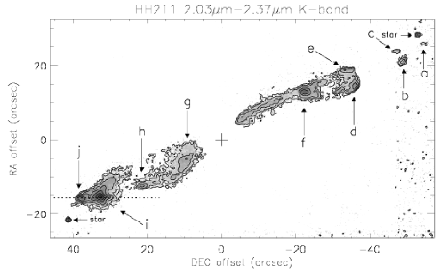
Figure 1: Broad-band K image of HH 211 which covers wavelengths between 2.03$\mu$m and 2.37$\mu$m. Features are labeled according to the nomenclature of McCaughrean et al. (1994). The exciting source HH 211-mm at position R.A.(2000) = 03^h 43^m 56.7^s, Dec(2000) = +32$\degr$ 00$\arcmin$ 50.3$\arcsec$ (Avila et al. 2001) is indicated by the cross. KSPEC spectroscopic slit positions are indicated by the dotted lines. Note that the star in the south-west of this image (and following images) has been masked for display purposes.

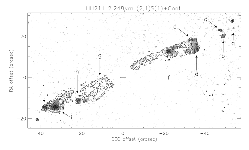
Figure 2: HH 211 at 2.248 $\mu$m. The grey-scale is the continuum subtracted image showing only the (2,1) S(1) line emission. Overlaid are contours representing the non continuum subtracted image. Thus the contours nearer the source trace predominantly scattered light while the contours further out mostly trace compact, line-emission features. The contour levels, which are scaled logarithmically, are at 0.22, 0.44, 0.87, 1.74, 3.47 $\times$ 10^-18 W m^-2 arcsec^-2.

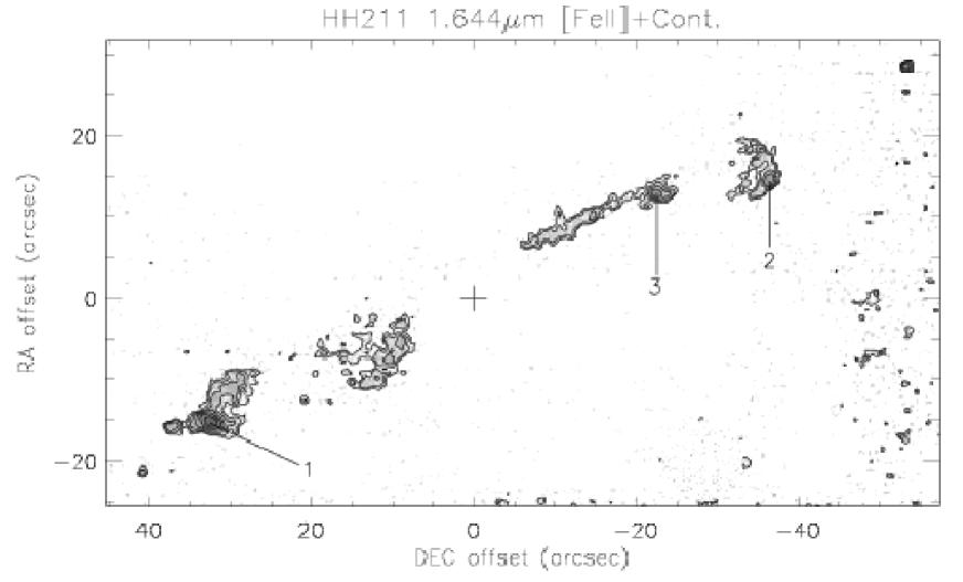
Figure 3: HH 211 at 1.644 $\mu$m. The greyscale and contours both trace the [FeII] line plus continuum emission. Consequently, most of the distributed flux can be attributed to continuum emission, although some concentrated condensations of [FeII] line emission are observed. These are labelled 1 –3. The logarithmic contours measure the flux at 0.63, 1.0, 1.58, 2.51, 3.98, 6.31 $\times$ 10^-19 W m^-2 arcsec^-2.

The NIR images were taken in November 1995 at the 3.5 meter telescope on Calar Alto using the MAGIC infrared camera (Herbst et al. 1993) in its high resolution mode (0.32″  per pixel). Images were obtained using narrow band filters centered on the H₂ (1,0) S(1) emission line at 2.122 $\mu$m, the (2,1) S(1) line at 2.248 $\mu$m, the (3,2) S(3) line at 2.201 $\mu$m and on the nearby continuum at 2.140 $\mu$m. The per pixel integration time was 1740s. Seeing throughout the observations was $\sim$0.9″except for the 2.14 $\mu$m image where it is $\sim$1″.8. The narrow-band image containing the (1,0) S(1) line has been previously published in Eislöffel et al. (2003).

The data could not be accurately flux calibrated due to non-photometric conditions. The total H₂ (1,0) S(1) flux from the entire outflow was previously measured to be 1.0 $\times$ 10^-15 W m^-2 by McCaughrean et al. (1994) which agrees with our flux calibration. We have deduced a calibration for all our narrow band images according to this measurement assuming that the average integrated flux from several bright unsaturated field of view stars should be similar for each filter. This should be the case because each filter FWHM is equal to 0.02 $\mu$m and the spectral energy distribution (SED) is likely to be relatively flat on average between 2.122 $\mu$m and 2.248 $\mu$m. We assume the accuracy of this method to be $\sim$15%.

2.3 UFTI observations

Further NIR observations of HH 211 were carried out on December 12, 2000 (UT) at the U.K. Infrared Telescope (UKIRT) using the near-infrared Fast Track Imager UFTI (Roche et al. 2003). The camera is equipped with a Rockwell Hawaii 1024 $\times$ 1024 HgCdTe array which has a plate scale of 0″.091 per pixel and provides a total field of view of 92″.9 $\times$ 92″.9.

Images in the [FeII] ⁴D_7/2 – ⁴F_9/2 transition were obtained using a narrow-band filter centered on $\lambda$ = 1.644 $\mu$m with $\Delta\lambda$(FWHM) = 0.016 $\mu$m). The outflow was also imaged using the broad-band K[98] filter centered on $\lambda$ = 2.20 $\mu$m with $\Delta\lambda$(FWHM) = 0.34$\mu$m. Seeing throughout the observations was $\sim$0″.8.  Nine-point ‘jittered’ mosaics were obtained in each filter.

Standard reduction techniques were employed (using the Starlink packages CCDPACK and KAPPA) including bad-pixel masking, sky subtraction and flat-field creation (from the jittered source frames themselves). The images were registered using common stars in overlapping regions and mosaicked. The observations were conducted under photometric conditions, so the faint standard FS11 (spectral type A3; H = 11.267 mag) (Hawarden et al. 2001) was also observed and used to flux calibrate the [FeII] image. The final images were smoothed using a circular Gaussian filter of FWHM = 0″.25.  in order to increase the signal to noise without compromising the resolution.

3 Results

Table 2: Photometric results for HH 211. The flux in units of 10^-18 W m^-2 is measured over the indicated circular apertures. Note that the measurements were made from images which are not continuum subtracted because of the low S/N of the continuum image. To infer the line emission fluxes the continuum values^∗ need to be subtracted. The (2,1) S(1)/(1,0) S(1) (labeled 2/1) ratios have been determined after subtracting the 2.14 $\mu$m continuum emission. In the case of knot g the (2,1) S(1) flux is equal to the continuum flux so no ratio was derived.

Knot	aperture	(1,0) S(1)†	(2,1) S(1)†	(3,2) S(3)†	2.14$\mu$m Cont.†∗	Broad-band K‡	[FeII] 1.644$\mu$m†	2/1 ratio
HH 211-west	57″	413	61	34	42	1285	28	0.05 (0.04)
HH 211-east	42″	575	98	63	55	2197	41	0.08 (0.03)
bow-a	5.3″	7.2	0.6	no det.	no det.	9	no det.	0.08 (0.04)
bow-bc	7.7″	32.0	2.3	no det.	no det.	65	no det.	0.07 (0.02)
bow-de	10.1″	155.5	18.1	7.3	3.1	335	11.8	0.09 (0.02)
b	4.9″	19.3	1.5	no det.	no det.	41	no det.	0.08 (0.02)
c	4.9″	11.2	0.9	no det.	no det.	21	no det.	0.08 (0.03)
d	6.0″	89.6	10.2	4.0	1.9	192	6.1	0.09 (0.03)
e	6.0″	57.5	7.9	3.3	1.3	131	4.8	0.12 (0.03)
f	10.1″	157.2	19.3	9.1	8.9	395	9.0	0.07 (0.04)
g	10.1″	41.9	20.6	20.6	19.6	380	14.3	–
h	10.1″	60.3	9.8	5.1	4.7	190	4.6	0.09 (0.08)
ij	17.9″	458.3	54.3	27.9	24.6	1364	25.0	0.07 (0.03)

^† The background 1$\sigma$ noise estimates over an 8″aperture are: 2.8 for H₂ (1,0) S(1); 0.2 for H₂ (2,1) S(1); 0.7 for H₂ (3,2) S(3); 1.1 for the 2.14$\mu$m continuum; and 3.4 for the [FeII] at 1.644$\mu$m, also in units of 10^-18 W m^-2.
^‡ As a standard star was not observed in the K[98] filter the broad-band fluxes are rough estimates. The flux calibration factor which we used was derived from the (1,0) S(1) calibration and a comparison of the broad-band and narrow-band filters.

Fig. 1 displays the HH 211 outflow in the K-band between 2.03$\mu$m and 2.37$\mu$m which contains all the K-band line emission as well as a large proportion of continuum emission. The principle knots have been labeled as in McCaughrean et al. (1994).

The H₂ (2,1) S(1) image is displayed in Fig. 2. The continuum at 2.14 $\mu$m has been subtracted in order to indicate locations of pure (2,1) S(1) emission (greyscale). Contours of the non continuum subtracted image are also displayed in order to indicate the extent of the continuum emission at 2.248 $\mu$m. The line emission is produced from an excitation level which is 12,553 K above the ground state whereas the (1,0) S(1) arises from 6,953 K. Therefore, we expect it to highlight the hotter parts of molecular shocks.

The western outflow shows particularly interesting structures which can be described as a series of bow shocks propagating along the outflow away from the source. Bows de and bc display a common asymmetric structure: the lower bow wing is approximately 1.5 times brighter than the upper wing. We will interpret this asymmetry in § 4 as due to a misalignment of the magnetic field with the flow through which the bow shock configurations with C-type flanks are propagating.

Emission detected at 1.644 $\mu$m is displayed in Fig. 3. Most of the emission detected here is attributed to the high level of continuum flux, as is seen in the K-band (Fig. 1). Steeply rising above this continuum level are several concentrated [FeII] emission condensations, labeled 1 – 3, one of which forms part of a well defined bow-shock, bow-de.

We confirm the existence of a band of continuum emission which extends along the western outflow. It becomes visible 5″  from the driving source and maintains a relatively constant flux out to 17″  from the source. Eislöffel et al. (2003) suggest that this continuum is scattered radiation from HH 211-mm which opens the possibility of indirectly obtaining a spectrum of the outflow source. The band of continuum is prominent in the K-band as well as at 1.644$\mu$m.

The photometric results for knots a – j are listed in Table 2. Knots d,e and b,c are interpreted as bow-shock components and are labeled as bow-de and bow-bc. We will briefly discuss the implications of these fluxes. The eastern outflow is $\sim$1.5 times brighter than the western outflow. However, the cause of this difference is not necessarily due to an unequal jet power output as Giannini et al. (2001) detected similar levels of OI 63 $\mu$m in both lobes (1.02 L_☉ in east; 0.94 L_☉ in west). This line is relatively unaffected by extinction and represents the main cooling channel in the post-shocked gas. The non photometric conditions during the observations are reflected in the relatively large 1$\sigma$ noise levels which have been estimated from the background flux variation using an 8″aperture. Most of the emission in the (3,2) S(3) image is actually continuum emission except possibly for bow-de. Interestingly, the fluxes at 1.644 $\mu$m are also comparable to the continuum fluxes. This implies that the dereddened continuum fluxes are 2 – 5 times brighter at 1.644 $\mu$m than at 2.14$\mu$m taking into consideration the higher extinction (A_H = 1.6 A_K), the range of extinctions explored (see below and § 5), and that the 1.644$\mu$m filter width is 25% narrower than the 2.14$\mu$m filter. The (2,1) S(1)/(1,0) S(1) ratios are calculated with the continuum subtracted. The error propagation results in very large errors at locations where the continuum forms a large fraction of the H₂ emission.

From the KSPEC data, we can extract several pieces of information. We calculate the differential extinction between two transition lines (in magnitudes) using

$$\Delta=2.512\,\log\left(\frac{F_{1}\lambda_{1}g_{2}A_{2}}{F_{2}\lambda_{2}g_{1}A_{1}}\right)$$ (1)

where $\lambda_{1}$ and $\lambda_{2}$ are the transition wavelengths, F₁ and F₂ are the relative fluxes, g₁ and g₂ are the upper level degeneracies, and A₁ and A₂ are the spontaneous electric quadrupole transition probabilities taken from Wolniewicz et al. (1998).

When both lines originate from the same upper level and a K-band spectral index of 1.7 is adopted, the absolute extinction is given by

$$A_{K}=\frac{\Delta}{\left[\left(\frac{2.2\mu m}{\lambda_{2}}\right)^{1.7}-\left(\frac{2.2\mu m}{\lambda_{1}}\right)^{1.7}\right]}.$$ (2)

Three pairs of H₂ $v$=(1,0) lines from the KSPEC data were used in order to determine A_K: Q(2)/S(0), Q(3)/S(1) and Q(4)/S(2). The results are presented in Table 3.

Table 3: A_K values (in magnitudes) which have been determined from the KSPEC relative fluxes in Table 1. The flux errors have been propagated and yield a realistic A_K error estimate.

	Q(2)/S(0)	Q(3)/S(1)	Q(4)/S(2)
AK east	2.7 $\pm$ 1.5	1.5 $\pm$ 0.5	1.8 $\pm$ 0.5
AK west	3.9 $\pm$ 2.3	2.4 $\pm$ 0.5	3.2 $\pm$ 2.0

Immediately evident is that the extinction is higher in the western knots although the extinction determination in the west is rather tentative due to the observing conditions. A higher extinction than in the east is plausible since the western lobe is redshifted and the embedded cloud (observed in H¹³CO⁺ by Gueth & Guilloteau (1999)) extends predominantly in this direction. In order to determine the average value of A_K each line pair was assigned with the relative line strength as a statistical weight. The statistically weighted average A_K values for the eastern and western components are 1.8 and 2.9 magnitudes respectively. These values fall within the error limits and are used to deredden luminosities in § 4.

In order to interpret the data, we employ the Column Density Ratio (CDR) method. We determine the column of gas, $N_{j}$, in the upper energy level, $k\,T_{j}$, necessary to produce each line. We then divide these values by the columns predicted from a gas at 2,000 K in local thermodynamic equilibrium with an ortho to para ratio of 3. Normalising to the (1,0) S(1) line, we then plot this as the CDR, as displayed in Fig. 4. We immediately see that the CDR is not constant but a function of excitation temperature, and thus is not consistent with emission from a uniform temperature region or from a single planar shock. Furthermore, no significant deviations from a single curve are identified (apart from that derived from the (1,0) S(5) which is not confirmed by the (1,0) Q(7) from the same $T_{j}$). Hence, the ortho to para ratio is consistent with the value of three, usually associated with H₂ shocks.

Figure 4: Column density ratio diagrams for HH 211, produced from vertical slits running through locations of peak emission. The extinction has been adjusted to minimise the differences in 1–0 S-branch and Q-branch lines originating from the same upper energy level. H₂ (1,0) transitions are represented by squares, (2,1) transitions by crosses, and (3,2), (3,1) and (3,0) transitions by triangles. The faint squares represent (1,0) Q branch measurements.

The extinction determined in the east location also constrains the H-band lines. A significantly lower extinction would raise the CDRs for these (1,0) H₂ above that of the (2,1) K-band lines which would have implied non-LTE low density conditions. As it stands, the fact that a single curve is predicted suggests a density sufficiently high to ensure LTE. Given a high fraction of hydrogen atoms, the lower vibrational levels of hydrogen molecules reach LTE at densities above $\sim$ 10⁴ cm^-3.

4 Analysis

4.1 Modeling the bow shocks

Figure 5: The HH 211 western outflow is shown here in H₂ (1,0) S(1), H₂ (2,1) S(1) and [FeII] emission lines. The images are not continuum subtracted as the bow shocks are relatively pure. Greyscale bars represent flux levels per arcsec^-2  in units of 10^-18 W m^-2.

The structure of the western outflow, shown in detail in Fig. 5, raises an ideal interpretation scenario. The excited H₂ can be found in several distinct knots along an outflow axis. McCaughrean et al. (1994) suggested that this well organised appearance might prove particularly amenable to modeling. A series of bow-shocks is propagating along the outflow. They gradually exhaust their momentum and slow down as they plough through either ambient gas or the material in the wakes of upstream bow shocks. They encounter less dense gas towards the edge of the cloud. The submillimeter observations of Chandler & Richer (2000) show that the HH 211-mm envelope density decreases with distance from the source. The azimuthally averaged density structure is well fitted by a single power-law,   $\rho\propto r^{-1.5}$, out to 0.1 pc (the projected distance of the outer knots of the outflow from the source). However, the density profile is extended in a direction perpendicular to the outflow and the outer western knots are located outside this dense core region.

The bow-shock models described by Smith et al. (2003) have been successfully employed to interpret the sequence of bow shaped features along the HH 240 outflow (O’Connell et al. 2004). Here we apply the same model which serves as a useful interpretive device. We wish to determine if a systematic change of one or more parameters results in a close match with the observed bow structures and thus to analyse the outflow’s changing environment. We have applied the bow-shock model to the three leading structures: de, bc and a.

Jump-type (J-type) bow shocks can explain many of the features associated with high excitation emission regions. They cause rapid heating and dissociate H₂ molecules for shock speeds greater than 24 km s^-1 (Kwan 1977). However, Continuous-type (C-type) bow shocks have proved extremely successful at interpreting most of the observed structures. The measured low fraction of ions in molecular clouds is consistent with their application. The magnetic field cushioning means that less energy goes into molecule dissociation; they can explain the high infrared fluxes which are observed in bow shocks. However, their observed velocities often exceed the H₂ dissociation speed of $\sim$ 40–50 km s^-1 (Smith et al. 1991) giving rise to a double-zone bow shock composed of (1) a curved J-type dissociative cap (responsible for atomic emission) and (2) C-type wings (where H₂ emission is radiated).

Our C-type bow shock model consists of a three dimensional curved surface described by

$$Z/L_{bow}=(1/s)(R/L_{bow})^{s},$$ (3)

where $Z$ and $R$ are cylindrical coordinates, $L_{bow}$ characterises the bow size and $s$ defines the shape or sharpness of the bow. The curved shock surface is then divided into a very large number of steady-state planar shocks for which the detailed physics and chemistry are computed (Draine 1980; Smith et al. 1991). Each mini-shock propagates at a different velocity depending on the angle between the shock surface normal and the direction of motion of the bow. The temperature reached, and hence the excitation conditions, depends on the shock velocity, density, magnetic field strength, etc., as well as the magnetic field direction (see Table 4).

Table 4: Model parameters derived to fit the bow images with C-type shocks.

Parameter	bow-de	bow-bc	bow-a
Size, $L_{bow}$ (cm)	1.0 $\times$ 1016	1.0 $\times$ 1016	1.0 $\times$ 1016
H Density, n (cm-3)	8.0 $\times$ 103	4.0 $\times$ 103	3.0 $\times$ 103
Molecular Fraction	0.2	0.2	0.2
Alfvén Speed, $v_{A}$ (km s-1)	4	4	4
Magnetic Field ($\mu$G)	193	137	118
Ion Fraction, $\chi$	1.0 $\times$ 10-5	3.0 $\times$ 10-5	5.5 $\times$ 10-5
Bow Velocity, $v_{bow}$ (km s-1)	55	40	29
Angle to l.o.s.	100∘	100∘	100∘
s Parameter	2.10	1.90	1.75
Field angle, $\mu$	60∘	60∘	60∘

Table 5: Observed and predicted bow shock luminosities and (2,1) S(1) / (1,0) S(1) flux ratios. Luminosities are expressed in units of L_☉ and a distance of 315 pc is adopted. Luminosities have been dereddened using K-band and H-band extinctions of 2.9 and 4.5 magnitudes (using A_H = 1.56 $\times$ A_K from Rieke & Lebofsky (1985)) although the errors in these values are relatively large, see table 3. respectively. Note that the [FeII] luminosities have been predicted using a J-type shock model.

Line	Observed∗	Dereddened	C-type
			Model
bow-de
H2 (1,0) S(1)	4.6 $\times$ 10-4	6.5 $\times$ 10-3	6.8 $\times$ 10-3
H2 (2,1) S(1)	4.3 $\times$ 10-5	6.1 $\times$ 10-4	7.3 $\times$ 10-4
H2 (3,2) S(3)	9.8 $\times$ 10-6	1.4 $\times$ 10-4	1.6 $\times$ 10-4
$[FeII]$   4D7/2 – 4F9/2	3.6 $\times$ 10-5	2.2 $\times$ 10-3	2.3 $\times$ 10-3
$\mathsf{2/1\leavevmode\nobreak\ \leavevmode\nobreak\ ratio}$	$\mathsf{0.09\,(0.02)}$	$\mathsf{0.09\,(0.02)}$	$\mathsf{0.11}$
bow-bc
H2 (1,0) S(1)	9.7 $\times$ 10-5	1.4 $\times$ 10-3	1.4 $\times$ 10-3
H2 (2,1) S(1)	6.85 $\times$ 10-6	9.7 $\times$ 10-5	1.5 $\times$ 10-4
H2 (3,2) S(3)	no det.∗	–	2.7 $\times$ 10-5
$[FeII]$ 4D7/2 – 4F9/2	no det.∗	–	1.2 $\times$ 10-4
$\mathsf{2/1\leavevmode\nobreak\ \leavevmode\nobreak\ ratio}$	$\mathsf{0.07\,(0.02)}$	$\mathsf{0.07\,(0.02)}$	$\mathsf{0.12}$
bow-a
H2 (1,0) S(1)	2.2 $\times$ 10-5	3.1 $\times$ 10-4	3.2 $\times$ 10-4
H2 (2,1) S(1)	1.7 $\times$ 10-6	2.4 $\times$ 10-5	2.5 $\times$ 10-5
H2 (3,2) S(3)	no det.∗	–	2.6 $\times$ 10-6
$[FeII]$ 4D7/2 – 4F9/2	no det.∗	–	1.2 $\times$ 10-6
$\mathsf{2/1\leavevmode\nobreak\ \leavevmode\nobreak\ ratio}$	$\mathsf{0.08\,(0.04)}$	$\mathsf{0.08\,(0.02)}$	$\mathsf{0.08}$

^∗The 3$\sigma$ detection limits for the observed knots over an 8″circular aperture are: 2.6 $\times$ 10^-5 for (1,0) S(1); 1.8 $\times$ 10^-6 for (2,1) S(1); 6.4 $\times$ 10^-6 for (3,2) S(3); and 3.1 $\times$ 10^-5 for the [FeII] image.

The systematic method of exploration of parameter space is given in O’Connell et al. (2004). In summary, the bow luminosities provide constraints on the density and bow speed. The location of the emission in the flanks or apex also constrains the bow speed. In addition, the ion fraction constrains the transverse bow thickness as well as the bow speed. The magnetic field strength strongly influences the extent of the wing emission and the atomic fraction affects the line ratios. As demonstrated by previous modelling, the bow speed is limited to within $\sim$ 15%, the orientation to within 10^∘ and the density, magnetic field, atomic fraction and ion fraction to within a factor of two.

The observed H₂ (1,0) S(1) luminosity for each bow provides us with the strongest density and velocity constraint. For a given bow size, L_bow, the line emission is directly proportional to the mass density (= 2.32 $\times$ 10^-24n_c) and ($v_{bow}$)³. The observed bow luminosities have been dereddened using a K-band extinction of A_K = 2.9 mag (see § 3). Table 5 lists the observed dereddened luminosities for each knot along with the predicted model luminosities.

The parameters selected in order to model each bow are given in Table 4. A constant Alfvén speed is maintained so that the magnetic field varies with density (B=$v_{A}$(4$\pi\rho$)^0.5). From the H₂ radial velocity structure described in Salas et al. (2003) and that the outflow H₂ knots have an average velocity projected onto the plane of the sky of $\sim$ 50 km s^-1 (such a velocity is consistent with our modelling results) we have estimated an inclination angle to the plane of the sky of between 5^∘ and 10^∘. The bows have been modelled propagating at this angle, i.e. 100^∘ to the line of sight as the western outflow is redshifted. At this angle the model images closely resemble the observations suggesting that the bow speed is similar to the shock speed, i.e the bows are propagationg in a medium which is relatively at rest.

The field angle, $\mu$, is the angle between the bow direction of motion and the magnetic field (see O’Connell et al. (2004) for a detailed description of the geometry). A misalignment of these directions results in asymmetric bow wings such as are observed for HH 211. In our case the best results were found for $\mu$ $\sim$60^∘$\pm$10^∘.

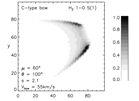
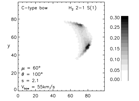
Figure 6: A C-type bow shock model for bow-de shown in H₂ (1,0) S(1) and (2,1) S(1) excitation lines. Adopting a source distance of 315 pc gives a pixel scale along the x and y axes of 1 pixel = 0″.18. The bow direction of motion is inclined to the plane of the sky by an angle of 10^∘, away from the observer, i.e. 100^∘ to the angle of sight. The bow is moving at 55 km s^-1 relative to the ambient medium of H density,n, = 8 $\times$ 10³ cm^-3. All flux levels are indicated normalised to the maximum H₂ (1,0) S(1) line flux. Hot dissociative shocks are necessary to induce emission from [FeII]. Here we have employed a J-shock model (same parameters) to simulate the flux distribution at 1.644 $\mu$m.

Fig. 6 displays the simulated bow image to compare to bow-de in (1,0) S(1) and (2,1) S(1) ro-vibrational transition lines of H₂, as well as the [FeII] ⁴D_7/2 – ⁴F_9/2 transition line. The shock speed is 55 km s^-1 and the pre-shock density is 8 $\times$ 10³ cm^-3. The bow size, L_bow, has been chosen in order to match the distance between the upper and lower wings, in this case $\sim$5″.

The [FeII] emission is generated by a J-type dissociative bow and is restricted to a compact but elongated zone towards the bow apex where the highest temperatures are reached. However, the observed [FeII] emission is restricted to a single compact condensation, unlike the model distribution. According to this model the total cooling in the (1,0) S(1) line is 6.8$\times$10^-3 L_☉, 1.4$\times$10^-1 L_☉ in all H₂ rotational and vibrational lines and 2.4$\times$10^-1 L_☉ in all atomic and molecular lines.

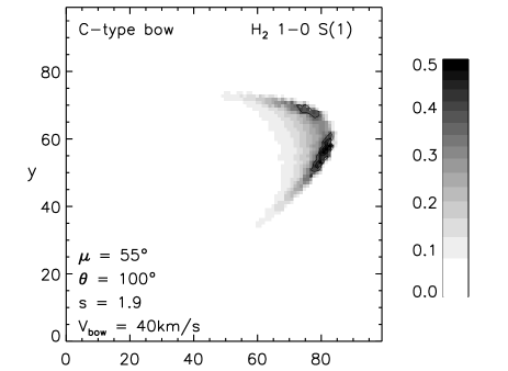
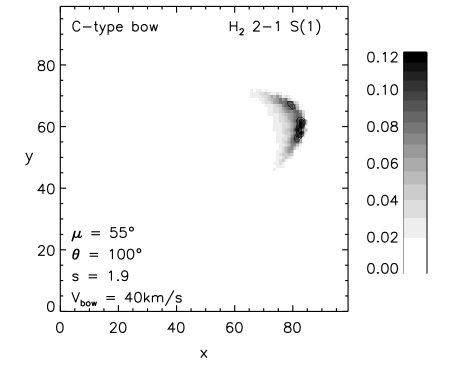
Figure 7: C-type bow shock model for bow-bc which reproduces the observed H₂ (1,0) S(1) and (2,1) S(1) flux distribution. Adopting a source distance of 315 pc gives a pixel scale of 1 pixel = 0″.18. Here we take a lower bow speed of 40 km s^-1 and a pre-shock H density of 4 $\times$ 10³ cm^-3 to match the observed luminosity. Other parameters are given in table 4. The grey scale flux indications are normalised to the maximum (1,0) S(1) level for bow-de in Fig. 6.

Bow-bc is observed in both the (1,0) S(1) and (2,1) S(1) lines. Fig. 7 displays the model generated images which closely resemble the observations. The distance between the upper and lower wings is $\sim$3″. This knot is modeled with a reduced bow speed of 40 km s^-1 which is propagating into a lower density medium (n = 4.0 $\times$ 10³ cm^-3. No [FeII] emission is observed, consistent with the fact that its predicted luminosity lies below the detection threshold. According to this model the total cooling in the (1,0) S(1) line is 1.4$\times$10^-3 L_☉, 3.6$\times$10^-2 L_☉ in all H₂ rotational and vibrational lines and 5.4$\times$10^-2 L_☉ in all atomic and molecular lines.

Bow-a appears in the (1,0) S(1) line as a compact knot of emission with a (2,1) S(1) / (1,0) S(1) ratio of 0.08 $\pm$ 0.02. A bow speed of 29 km s^-1 results in emission restricted to the bow apex. The calculated line cooling is 3.2 $\times$ 10^-4 L_☉ in the (1,0) S(1) line, 8.8 $\times$ 10^-3 L_☉ in all H₂ lines and 1.3 $\times$ 10^-2 L_☉ total line cooling.

Figure 8: Faint (1,0) S(1) emission is detected at bow-a. A bow propagating at 29 km s^-1 generates the correct (1,0) S(1) luminosity with luminosities from the other lines below the level of detectability, see table 5. Adopting a source distance of 315 pc gives a pixel scale of 1 pixel = 0″.18. The grey scale flux indications are normalised to the maximum (1,0) S(1) level for bow-de in Fig. 6.

We conclude that the observed structures are recreated in the model by solely altering the density, bow speed and ion fraction while all other parameters remain fixed. The extent of the bow is influenced principally by the bow speed as it determines the location of the H₂ emission. A slower bow is characterised by emission concentrated closer to the bow front. For this reason we have maintained a constant L_bow for all the models. The bow speed systematically decreases as an otherwise similar bow ploughs into a material of decreasing density. An increase in the ion fraction is expected in less dense regions where cosmic rays and UV photons can more easily penetrate the gas.

The driving power of a bow is converted into heat at a theoretical rate $P=\zeta\rho v_{bow}^{3}L_{bow}^{2}\pi/2$ or

$$P=0.13\zeta\biggl{(}\frac{n}{8.0\times 10^{3}\leavevmode\nobreak\ {\rm cm}^{-3}}\biggr{)}\biggl{(}\frac{v_{bow}}{55\leavevmode\nobreak\ {\rm km\leavevmode\nobreak\ s}^{-1}}\biggr{)}^{3}\biggl{(}\frac{L_{bow}}{1.0\times 10^{16}\leavevmode\nobreak\ {\rm cm}}\biggr{)}^{2}{\rm L}_{\sun},$$ (4)

where $\zeta$ is a non-dimensional factor related to the aerodynamical drag and is of order unity. $\rho$ is the mass density equal to $2.32\times 10^{-24}n$ ($n$ is the hydrogen nucleon density). The derived numbers are thus consistent with expectations.

4.2 The outflow continuum emission and excitation

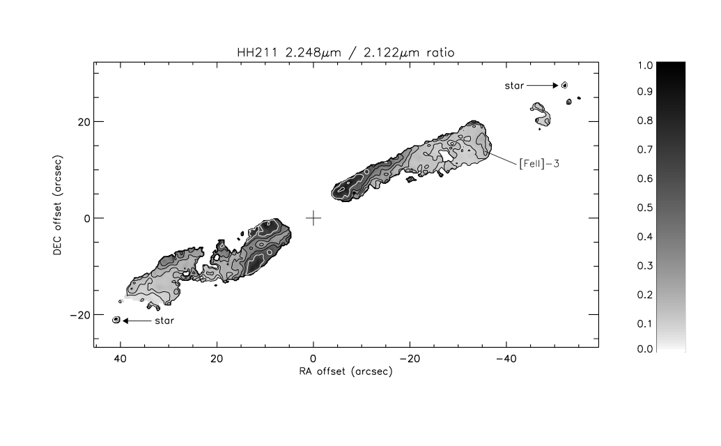
Figure 9: A map showing the ratio of our 2.122$\mu$m and 2.248$\mu$m images. The two images have not been continuum-subtracted (due to the very low S/N of the continuum image), so the map only reveals the H₂ (2,1) S(1)  / (1,0) S(1) line ratio towards the ends of the outflow, where the continuum is weak; the darker regions near the center of the image are where the emission is dominated by the continuum. Logarithmically increasing contour levels are at 0.08, 0.11, 0.16, 0.22, 0.32, 0.45 (black) and 0.63, 0.89 (white).

We have also divided the fluxes in the narrow-band images containing the (1,0) S(1) flux and the (2,1) S(1) flux to produce the ratio image displayed in Fig. 9. In order to produce this map both images were first smoothed with a Gaussian FWHM = 0″.6 and values lying below the noise level were excluded before dividing. Note that the images were not continuum subtracted, due to the poor quality of the continuum image at 2.14$\mu$m, so Fig. 9 reveals two distinct outflow regions: (1) areas where the continuum emission is relatively strong possess a ratio above 0.3 and approach 1.0 where only continuum emission is present and (2) parts of the outflow not effected by continuum emission where the H₂ excitation ($\sim$ 0.1) can be studied.

The outflow regions dominated by continuum emission are located along the edges of the SiO jet imaged by Chandler & Richer (2001). This supports the idea that the continuum arises through scattered light from the protostar. The light escapes along a jet excavated cavity but not along the high density jet itself. It is cut off at 17″(8.0 $\times$ 10¹⁶ cm) along the western outflow where it possibly encounters a high density 1 M_☉ filament (Gueth & Guilloteau 1999). It is also possible that the filament lies in front of the flow. This projection effect would explain the higher extinction measured in the western outflow, contrary to the submillimeter dust emission maps of (Chandler & Richer 2000) which do not reveal a strong asymmetrical density distribution between the eastern and western outflows. Continuum light encounters less hindrance along the eastern outflow where it terminates alongside shock excited H₂ emission at knots i and j, 45″(2.1 $\times$ 10¹⁷ cm) from its protostellar origin. Here continuum emission is seen at 2.14$\mu$m (Eislöffel et al. 2003) but not in our ratio image as the H₂ emission is relatively strong here. The origin and implications of the continuum emission will be discussed in § 5.

The excitation ratio along the western outflow,$\sim$ 0.1, is typical of outflows seen in collisionally excited emission (Black & Dalgarno 1976; Shull & Beckwith 1982). There is an increase in the excitation ratio towards the leading edge of bow-de where higher shock velocities and temperatures are reached and the H₂ line emission reaches its maximum value. Similar conditions were found for the HH 240 bow shocks (O’Connell et al. 2004) and they are well explained through the bow shock interpretation. However, a strong deviation from this picture is found in the [Fe II] image: The localised [FeII] emission is coincident with a region of higher ratio, (labelled [FeII]–3) and, puzzlingly, not at the expected H₂ dissociated bow apex as seen in the model generated image, Fig. 6.

5 Discussion

Which mechanisms give rise to the series of near-infrared bow shocks? Our analysis suggests a combination of two processes:

(1) The bow shocks are generated by a series of similar outflow accretion/ejection events. Using the model velocities the time lapses between the bows (and therefore between outflow events) are $\sim$ 425 and $\sim$ 290 years. These numbers are consistent with the detection of three bows given the dynamical age of $\sim$ 1000 years. Fluctuations in jet activity probably manifest themselves as bow shocks at the jet cloud impact region which is Knot-f where the high speed CO jet terminates and H₂ shock heating is initialised. At Knot-f two H₂ (1,0) S(1) velocity components have been observed by Salas et al. (2003). This reverse/transmitted shock pair seems to indicate the critical zone of jet impact where H₂ bow shocks are born. After formation, the bows propagate away from the protostar towards the cloud edge and through a changing environment; they become less luminous as the density decreases and they loose their momentum. Bow-a represents the final stages in the detectable life of one of these bow shocks. In support of this process, we note that the molecular jet demonstrates an apparent acceleration along its length of value $\sim$ 5 $\times$ 10^-3 km s^-1 AU^-1 (Chandler & Richer 2001). Given ballistic motions, this implies that the entire jet now observed was ejected within a relatively short period of time just 100–150 years ago.

(2) The bow shocks become illuminated within regions where the outflow impacts on denser clumps of gas. This idea is supported by the implied high K-band extinctions of 2.9 and 1.8 magnitudes for knots de and i. These values do not represent the entire outflow and cannot be used to infer the dereddened luminosity for the whole outflow. Additionally, strong continuum emission is detected in the eastern outflow at knots i and j where the extinction is high (A_K $\sim$ 1.8). If this is indeed scattered light from the protostar then it has channeled through to where the enhanced density has resulted in scattering. The passage of a C-shock will increase the post-shock density with a compression ratio of $\sqrt{2}$ times the magnetic Mach number (shock speed divided by the Alfvén speed) (Spitzer 1978). Therefore, the continuum emission is likely to be seen alongside the shock excited H₂ emission as is the case for HH 211.

McCaughrean et al. (1994) suggested an average A_K of 1.2 magnitudes which is lower than the values that we derived in § 3 but is consistent to within our error limits. Adopting this as the average extinction over the entire outflow we find that the total H₂ (1,0) S(1) luminosity of the entire outflow is 0.009 L_☉. According to the predictions of our bow shock models, $\sim$ 4% of the total H₂ line emission (2.7% of total line cooling) is emitted in the (1,0) S(1) which gives an intrinsic H₂ luminosity for HH 211 of $\sim$ 0.23 L_☉ and a total luminosity, L_rad, resulting from all line emission of $\sim$ 0.34 L_☉. If all the mechanical energy is converted into radiation then L_mech is equivalent to L_rad and L_mech / L_bol $\sim$ 10%.

Provided that the velocity of the swept up gas, which coincides with the CO outflow, roughly equals the shock velocity (i.e. a radiative shock), Davis & Eisloeffel (1996) have shown that L_rad should be roughly equal to the kinetic luminosity L_kin of the outflowing material as measured through the CO luminosity. These criteria are indeed met for HH 211 as L_kin $\sim$ 0.24 L_☉ and the CO and H₂ are coincident suggesting that the shock is essentially radiative (Gueth & Guilloteau 1999; Giannini et al. 2001). Note that the average extinction is restricted to about 1 magnitude in the K-band in order to meet these criteria.

The driving source HH 211–mm has a bolometric temperature of 33K which implies a youthful outflow system. However, the HH 211 outflow itself does not reveal any characteristic signs of its assumed youthfulness besides the small spacial extent which implies a dynamical timescale of order 1000 years. This outflow age is limited by the density structure of the environment, as older bow shocks may simply have disappeared into sparse material. For this reason the outflow extent itself cannot be used to infer the full duration of outflow activity.

The high density jet (2–5 $\times$ 10⁶ cm^-3) observable in SiO J = 5$\rightarrow$4 emission implies a pre-shock density of about 2 $\times$ 10⁵ cm^-3 (Gibb et al. 2004) and thus a maximum jet-to-ambient density ratio of $\sim$20. The CO J = 2$\rightarrow$1 maximum radial velocity is $\sim$ 40 km s^-1 (Gueth & Guilloteau 1999) implying a jet velocity of 230 – 460 km s^-1 given an inclination angle to the plane of the sky of between 5^∘ and 10^∘. Hydrodynamic numerical simulations find that a low density envelope generally develops around jets of density $\sim$ 10⁵cm^-3 and a jet-to-ambient density ratio of 10 (Suttner et al. 1997; Völker et al. 1999; Rosen & Smith 2004). Could (pulsed) C-type jets which are heavier, denser and more ballistic than those simulated excavate low density cocoons through which continuum emission might escape along the outflow? To date, such high density and high velocity jets involving C-type physics have not been simulated. The new challenge for theorists is to simulate such MHD jets.

HH 211 is of particular interest due to its unusually strong continuum emission. The original radiation may have escaped from the source along a cavity of low optical depth which must have been excavated by powerful jet events. This radiation is then scattered when it encounters dense walls or clumps where the NIR optical depth along the direction facing the source is of order unity. Some of the scattered radiation then exits along the line of sight through a foreground of moderate NIR extinction. This interpretation thus requires the original radiation to penetrate a distance of order 10¹⁷ cm with a mean density of less than 10⁵ cm^-3 before encountering walls of thickness of order 10¹⁶ cm and density 10⁶ cm^-3. A moderate fraction of the scattered radiation then escapes without encountering further dense features along the line of sight. The high density and clumpiness of the jet as revealed through SiO observations (Chandler & Richer 2001; Nisini et al. 2002) are important factors to consider in this interpretation.

The [FeII] emission at 1.644 $\mu$m originates from an upper energy level of 11,300 K (compare to 6,953 K for H₂ (1,0) S(1)) therefore we expect it to highlight the hotter, high excitation regions of an outflow. As shown in § 4, the [FeII] emission from a typical bow shock should be located towards the front of the bow, where H₂ is dissociated. Clearly, this is not the case for HH 211 (bow–de). The most likely explanation is that the front of the bow shock is traversing a low density region. Material has been swept out by outflow activity and the bow shocks become luminous only where they interact with the wall of this hollowed out cavity. In this way it is possible see [Fe II] emission coincident with bright H₂ emission in the ‘shoulders’ of the bow shock. Such an explanation is also supported by the distinct possibility that continuum emission from the source is escaping along an outflow excavated cavity.

6 Conclusions

We have studied the HH 211 protostellar outflow in the near-infrared regime through high resolution imaging and spectroscopy. Images in the (1,0) S(1) and (2,1) S(1) ro-vibrational transitions of H₂ have been analysed in order to study the excitation throughout the outflow. A narrow-band image at 1.644$\mu$m was presented where the outflow is clearly seen and several confined condensations of emission are identified. In addition, we have presented K-band spectroscopic fluxes for two separate prominent locations from which the extinction and excitation conditions have been investigated. We have successfully modeled the series of bow-shocks in the western outflow as curved 3–dimensional shock fronts with steady state C–type physics.

Our findings have lead to several conclusions about the nature of the outflow:

• C-type bow shocks propagate along the western flow. Model fitting has constrained several parameters including the density, bow velocity, ion fraction, intrinsic bow shape and magnetic field strength and direction.

• The bow shocks are passing through dense clumps where their luminosity is accentuated. High values of extinction are measured in these regions.

• Bows de, bc and a are plausibly modeled as a series of initially identical bow shocks propagating through a medium of decreasing density. The bows slow down and disappear as they approach the cloud edge.

• A misalignment of the magnetic field and outflow directions can account for the observed bow shock asymmetries.

• The most likely source of the protracted continuum emission is light from the protostar which evades dense core obscuration by escaping through a low density cavity excavated by the jet, as discussed in § 5. The continuum light is scattered when it encounters the denser material aligning the jet tunnel and the dense clumps along the outflow.

• The excitation along the outflow is typical of outflows in general. The ortho to para ratio of 3 for molecular hydrogen implies shock heating as the source of the near-infrared line emission.

• The [FeII] emission is predicted and detected in isolated condensations. These condensations are coincident with strong H₂ emission. However, the location of the [FeII] emission is puzzling; it is not found in the expected bow apex region as predicted. This may also be due to the low density tunnel through which the bow apex is propagating.

These findings together with the large volume of previously published material is suggesting a global outflow model, as follows. Episodic fluctuations in accretion/ejection (of order a few hundred years) give rise to a variable jet velocity. The resulting shocks manifest themselves as C-type bow shocks at the principle jet/ambient medium impact region where they are detected outside the dense core where the extinction is lower. The bows propagate towards the cloud edge through a changing environment. The model suggests that the mean density decreases with distance from the core but that the bow shocks brighten where they encounter dense clumps. It is feasible that these clumps consist of gas swept up by passage of previous bows driven by the alternating outflow power.

It is clear that in-depth studies of a wide range of protostellar outflows will yield valuable insight into how the cloud environment sculpts the outflow and how much the environment itself has been influenced by the star forming process.