Design of the Gaia photometric systems for stellar parametrization using a population-based optimizer

Abstract

Large, deep surveys must typically rely on multiband photometry rather than spectroscopy for determining the astrophysical properties (APs) of stars. Yet designing an optimal photometric system for a wide range of objects is complex, because it must trade off conflicting scientific requirements. I present a new method for designing photometric systems and apply it to the Gaia Galactic survey satellite, which will observe one billion stars brighter than V=20. The principle is to optimally sample stellar spectra in order to best determine the APs (e.g. ${\rm T}_{\rm eff}$, [Fe/H], interstellar extinction). By considering a filter system as a set of free parameters (central wavelengths, FWHM etc.), it may be designed by optimizing a figure-of-merit (FoM) with respect to these parameters. The FoM is a measure of how well the filter system can vectorially ‘separate’ stars in the data space to avoid AP degeneracies. The resulting systems show some interesting features, in particular broad, overlapping filters, which may be desirable from a multivariate classification perspective. These systems are competitive with others proposed for Gaia.

1 Introduction

Surveys of large numbers of objects will often be forced to employ photometry rather than spectroscopy due to confusion and SNR considerations. Given well defined scientific goals, the designer must decide how many filters to use, with what kind of profiles, where to locate them in the spectrum and how much integration time to assign to each. This is usually achieved via a manual inspection of typical target spectra. But if the survey is intended to establish multiple astrophysical parameters (APs) across a large and varied population of objects, then this method is unlikely to be very efficient or even successful. Even if a reasonable filter system could be constructed in this way, we would not know whether a better filter system exists subject to the same constraints. In this contribution I outline a more systematic approach to designing filter systems by optimizing a figure-of-merit (FoM) with respect to a parametrization of the filter system. The FoM is a measure of how well the filter system can ‘separate’ stars with different APs. This separation is vectorial in nature, in the sense that the local directions of AP variance are preferably mutually orthogonal to avoid AP degeneracy. I apply this model, HFD (Heuristic Filter Design), to the design of the photometric system for the Gaia mission. HFD and results of its application are described in more detail in Bailer-Jones (2004a,b).

2 Evolutionary Algorithms

Evolutionary Algorithms (EAs) are stochastic population-based optimizers which use principles of evolutionary biology to perform a directed search (e.g. Goldberg 1989). A population of individuals (candidate solutions) is evolved over many generations (iterations) making use of specific genetic operators to modify the genes (parameters) of the individuals. The goal is to locate the maximum of some fitness function (figure-of-merit). As a population-based method, it takes advantage of evolutionary behaviour (breeding, natural selection, maintenance of diversity etc.) to perform more efficient searches than single solution methods. The algorithm works iteratively: starting from some initial population, the fitness of each individual is calculated. A selection operator is then applied, in which individuals reproduce with a probability proportional to their fitness, i.e. fitter individuals produce more offspring. These offspring are produced by applying small random changes to the parents (mutation). This forms the next population and the procedure is iterated, as shown in Fig. 1.

Figure 1: The iterative loop (one iteration) of HFD.

3 Method

A filter system consists of $I$ filters. Each filter is parametrized with three parameters: the central wavelength, $c$, the half-width at half maximum (HWHM), $b$, and the fractional integration time, $t$, per star allocated to this filter. (The total integration time per star over the whole mission is fixed.) The profile shape of the filter is fixed. The optimization is performed with respect to these $3I$ free parameters.

The purpose of a filter system is to enable us to determine multiple stellar astrophysical parameters (APs), such as ${\rm T}_{\rm eff}$, [Fe/H] etc. To achieve this, the filter system must maximally separate stars with different APs. A suitable measure of this is defined as follows.

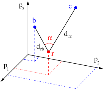
Figure 2: The fitness measures the separation between different types of stars as well as the angle between the directions in which the astrophysical parameters vary.

Given a fixed grid of stellar spectra, we synthesize the photometry for each of these stars in a given filter system and thus determine where they lie in the $I$-dimensional data space. At any point in this space, each AP will vary in a certain direction (the principal direction), and at a certain rate, the (scalar) AP-gradient. Fig. 2 shows an example for $I=3$. A good filter system will have large AP-gradients, i.e. a given pair of stars will be separated by a large amount (in proportion to their AP difference). This is necessary but not sufficient: We must also ensure that the angles between the principal directions are as near to 90^∘ as possible, to minimize the degeneracy between APs. The fitness of a filter system is a function which reflects these (for details see the box Fitness: the maths).

It is important to realise that the fitness is calculated using a specified grid of spectra. This grid (and the APs which vary in it) represents the types of objects we want the filter system to parametrize. In the example which follows, the grid shows variance in ${\rm T}_{\rm eff}$, $\log g$, [Fe/H] and A_V over relatively large ranges.

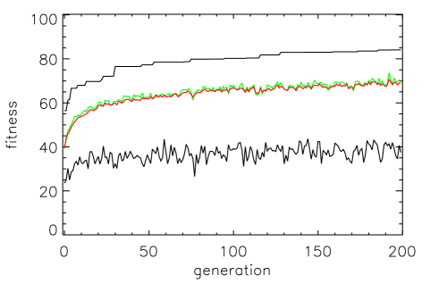
Figure 3: Fitness evolution of a population, showing (from top to bottom) the maximum, mean, median and minimum fitnesses.

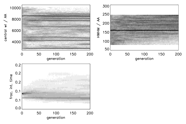
Figure 4: Evolution of the filter system parameters for systems with 12 filters, shown for all 200 filter systems (‘individuals’) in the population. At each generation all $12\times 200$ corresponding parameters are plotted (as a density grey scale, i.e. darker is a higher density).

Fitness: the maths The spectral grid shows variance in $J$ astrophysical parameters (APs). For each star, $r$, in the grid, we find its $J$ nearest neighbours, each of which differs from $r$ in only one of the $J$ APs. The relevant ‘distance’ between $r$ and that neighbour differing in AP $j$ (call it $n_{j}$), is the AP-gradient and is defined as $$h_{r,n_{j}}=\frac{d_{r,n_{j}}}{|\Delta\phi_{r,n_{j}}|}$$ where $d_{r,n_{j}}$ is the Euclidean distance between $r$ and $n_{j}$ in SNR units and $\Delta\phi_{r,n_{j}}$ is their difference in AP $j$. Clearly, the larger $h$ the better we have separated $r$ and $n_{j}$. To minimise the degeneracy between the principal directions to these $J$ neighbours we want angle $\alpha$ in Fig. 2 to be as close to 90∘ as possible for all neighbour pairs. Combining these measures, we see that a useful figure-of-merit of separation is $$x_{r,j,j^{\prime}}=h_{r,n_{j}}\,h_{r,n_{j^{\prime}}}\,{\sin\alpha_{r,j,j^{\prime}}}$$ where $j$ and $j^{\prime}$ label those neighbours which differ from $r$ in APs $j$ and $j^{\prime}$ respectively. (This is the magnitude of the cross product between the two vectors.) For $J$ APs we have $J(J-1)/2$ pairs of neighbours and thus $J(J-1)/2$ terms like that above, Summing these over all stars in the grid gives the final fitness, which is to be maximized $$F=\sum_{j,j^{\prime}\neq j}\sum_{r}x_{r,j,j^{\prime}}\ \ \ .$$ (The actual fitness function is a slight modification of this. See Bailer-Jones (2004) for details.)

4 Results

HFD is applied to design the Gaia photometric system. The optimization is performed within specified limits on the wavelength coverage of any filter plus maximum and minimum values of the HWHM of the filters As an example, an optimization is performed with 12 filters. A population size of 200 is used and is evolved for 200 generations. Multiple runs are performed with different initial (random) populations. An example of the evolution of the fitnesses in the population is shown in Fig. 3; the corresponding evolution of the filter system parameters is shown in Fig. 4. From each of many runs such as these, the best filter system is selected. Examples are shown in Fig. 5.

Figure 5: Five HFD-optimized filter systems. HFD also optimizes the integration time allocated to each filter. To show this the filter transmission curves have been multiplied by their fractional integration times (with the result that the intercepts of the profiles are not accurately depicted). The true filters all have a peak transmission of 0.9.

5 Conclusions

Various filter systems have been produced with HFD for Gaia. The best have a performance competitive with or better than conventionally-designed systems. One proposed for Gaia is shown in Fig. 6. Many optimization with different parameter settings have been carried out. General conclusions from this work are as follows:

• HFD often shows a preference for broad, overlapping filters. These may have advantages over traditional systems as they may make a better use of a high dimensional data space. (AP signatures are coherent over a wide wavelength range so broad filters can in principle still be sensitive to AP variations – see Fig. 7.)

• There is a trade-off between broad and narrow filters: narrower filters degrade the ‘scalar’ separation (as they achieve lower SNR) but improve the ‘vector’ separation (better at isolating the effects of APs).

• Some filters are placed very consistently, especially at the very blue and red ends. The wavelength space is not uniformly populated with filters, e.g. there is often a crowding around 7500–9000 Å.

• HFD shows a good ability to converge on a common filter system, but as the number of filters increases, there is less convergence. Although the different optimal filter systems show quite different properties, they achieve similar performance. In other words there are many different ‘good’ filter systems (roughly equal local optima).

HFD is a systematic and powerful approach to designing filter systems for surveys. Its principles are generic and it may be applied to many other survey projects.

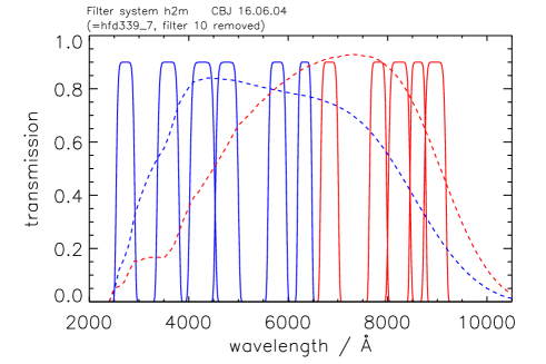
Figure 6: An 11-band system designed by HFD for stellar parametrization, and proposed for Gaia.

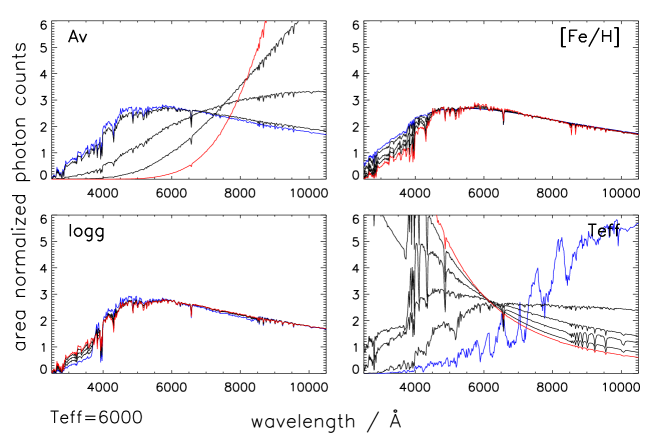
Figure 7: Examples of the effects that varying the four astrophysical parameters (APs) have on the spectra. (Each panel shows the effect of varying just the AP labelled.) The effect of APs is often coherent over over a wide wavelength range, meaning that broad (and overlapping) filters can be used for stellar parametrization, as found by HFD.

References

- (1) Bailer-Jones, C.A.L., 2004a, A&A 419, 385
- (2) Bailer-Jones, C.A.L., Gaia working group report, GAIA-CBJ-016
- (3) Goldberg, D.E., 1989, Genetic algorithms in search, optimization, and machine learning, Addison-Wesley, Reading, MA