Object classification and the determination of stellar parameters

Abstract

Gaia will observe more than one billion objects brighter than $G=20$, including stars, asteroids, galaxies and quasars. As Gaia performs real time detection (i.e. without an input catalogue) the intrinsic properties of most of these objects will not be known a priori. An integral part of the Gaia data processing is therefore to classify everything observed. This will be based primarily on multiband photometry provided by Gaia, but should also make optimal use of the high resolution spectroscopy (for brighter stars) and the parallaxes. In addition to a broad classification, we can also determine fundamental stellar parameters, in particular effective temperature, metallicity and the line-of-sight interstellar extinction. Such information will be essential for fully exploiting the astrometric part of the Gaia catalogue for stellar population studies. However, extracting this information is a significant challenge, and will need to make use of appropriate multidimensional data analysis techniques. I outline some of the problems and the strategies being developed to tackle them.

1 Introduction

The general astrometric principle of Gaia is similar to that of Hipparcos. It scans the sky with a pre-defined scanning law measuring the relative positions of objects. However, the two missions are fundamentally different in various ways, one of the most relevant being that Gaia goes much deeper, namely to about $G$ = 20 rather than $H_{p}$ = 12.4 as with Hipparcos. Thus whereas Hipparcos had an input catalogue, Gaia performs real-time onboard detection. Consequently, we generally have very little prior information about the targets which Gaia observes.

For this reason, Gaia is equipped with multiband CCD photometry in order to characterize its targets. As described elsewhere in these proceedings, this consists of 4–6 broad band filters in the Astrometric instrument, and around 12 medium band filters in the Spectroscopic instrument.

The main scientific goal of Gaia is to study the composition, origin and evolution of our Galaxy. Its main contribution to this topic is establishing very accurate stellar distances and 2D (or 3D) space motions, enabling us to study the 3D spatial structure and 3D kinematic phase space of different types of stars in the Galaxy. However, such information is of limited use if it cannot be associated with the intrinsic physical properties of these stars, in particular their abundances, masses and ages (or evolutionary state). Hence Gaia is not “just” about producing a catalogue of highly accurate astrometry and multiband photometry on hundreds of millions of stars. An integral part of the mission and data processing is to add essential scientific value to these by providing fundamental physical information on the targets. The challenge is to design a classification system – and develop appropriate algorithms – which can take the heterogeneous Gaia data and extract reliable estimations of the classes of objects and their physical parameters. This article gives a brief outline of the goals, requirements and issues facing this work.

2 Overall requirements and
available data

The main objectives of the classification are as follows

Discrete Source Classification

Determination of whether an object is a star, galaxy, quasar or asteroid etc. This could also include the use of morphological information.

Estimation of Astrophysical Parameters (APs)

For those objects identified as stars, determine their intrinsic physical properties. The relevant (and obtainable) ones are effective temperature, ${\rm T}_{\rm eff}$, surface gravity, $\log g$, metallicity, [Fe/H], and line-of-sight interstellar extinction, A_V. Although this last one is of course not intrinsic to the star, we would ideally determine it on a star-by-star basis, so we can consider it as such. Other APs of interest (and which could be determined for bright stars with the spectroscopy from the RVS instrument) include: alpha-process elements, [$\alpha$/Fe], CNO abundance anomalies, the microturbulence velocity, rotational velocity and activity.

Identification of unresolved binaries

Most stars are in multiple systems. Some of these can be recognised from the astrometry, and a few will be visual binaries, but most will go undetected in this way. Nonetheless, with favourable brightness ratios, a binary could be detected from the shape of its composite spectral energy distribution. This is important for determining the stellar mass function (as opposed to the system mass function) and for investigating the evolution of stellar clusters.

Identification of new types of objects

The history of astronomical discovery shows that new instruments, surveys and data analysis techniques lead to new, unexpected discoveries. Thus with Gaia we must be open to the prospect of detecting new types of objects (summarized by the cliche “expect the unexpected”.) This includes new types of variable stars, rare stars (e.g. brief phases of stellar evolution), abnormal abundance patterns or multiple systems. Those supervised classification methods which are commonly used for determining stellar parameters from spectra are generally forced to classify new types of objects into pre-existing classes. New objects would therefore go undetected (and samples of known types of objects would be contaminated). Thus special attention, including the use of unsupervised methods, is required to deal with this.

These classification tasks must rely mostly on the photometric data, as only these extend to the magnitude limit of Gaia’s onboard detection and thus astrometry. But recall that the photometry is obtained in two separate instruments, BBP and MBP. Only the former is obtained at the same spatial resolution as the astrometric data. Thus in sufficiently crowded fields we will only have BBP data, that is between 4 and 6 broad photometric bands. For bright stars, say brighter than $V=15$, we will also have reasonable quality RVS spectra, which will add considerable information, in particular on detailed abundances, peculiarities, rapid rotation and so forth. Finally, the parallaxes will of course also be valuable, as discussed in the next section.

3 Stellar astrophysical parameter estimation

The most fundamental properties of a star are its mass, age and chemical composition. Of course, age is not directly observable and masses can only be determined directly (i.e. dynamically) in select binary systems. Thus we must rely on indirect atmospheric indicators which can be obtained from the spectral energy distribution (SED). In particular, we are interested in the effective temperature, ${\rm T}_{\rm eff}$, surface gravity, $\log g$ and the iron-peak metallicity, [Fe/H]. Combined with the parallax and interstellar extinction, the luminosity, radius and mass can be determined.

non-astrometric parametrizer:
nSED, (RVS)	$\Rightarrow$	${\rm T}_{\rm eff}$, $\log g$, [Fe/H],
		A($\lambda)$, BC, [$\alpha$/Fe]?	atmospheric model
additional use of astrometry gives:
SED, BC, $\pi$, A($\lambda)$	$\Rightarrow$	L	$2.5\log L-f(\rm{SED,BC})$
			$=A-5\log{\pi}$
L, ${\rm T}_{\rm eff}$	$\Rightarrow$	R	$L=4\pi R^{2}\sigma T_{\rm eff}^{4}$
$\log g$, R	$\Rightarrow$	M	$g=GM/R^{2}$
SED, RVS, v(t), r(t)	$\Rightarrow$	detect unresolved binaries	orbital model
SED(t), RVS(t)	$\Rightarrow$	detect variables	variability model

Table 1: Stellar parameters derivable from the Gaia data. SED=spectral energy distribution (ca. 15 photometric measures in medium and broad band filters); nSED=normalized SED (absolute flux information removed); RVS=radial velocity spectrum; BC=bolometric correction; $\pi$=parallax; A($\lambda)$=interstellar extinction function; v(t) & r(t)=point source velocity and position as a function of time (from c. 85 observations over five years).

Most work on stellar parametrization has relied on relatively high resolution spectra from which ${\rm T}_{\rm eff}$, $\log g$ and [Fe/H] have been determined. Gaia is rather different in that it observes at lower spectral resolution but measures absolute fluxes as well as parallaxes. Table 1 shows how stellar parameters can in principle be derived from these data. The distance measurement accuracy for V = 15 is 1% at 1 kpc and 5% at 5 kpc. At V = 18 these are about 4% and 20% respectively. (These improve by a factor of two or more for late-type or very reddened stars.) Thus some 20 million stars will have their distances determined to better than 1% and have high precision SEDs. If ${\rm T}_{\rm eff}$ can be established to 1% then the radii of many of these stars is determinable to within 2%. If $\log g$ can be measured to 0.2 dex, then provided R (radius) can be established to within 10%, a mass determination to within 50% is possible without calibration from binary systems. Although poor for an individual star, it becomes statistically meaningful for a large sample of similar stars, which is where Gaia’s strength lies. Better individual masses will be possible from calibration using the tens of thousands of visual binaries observed by Gaia for which masses should be obtained to within 10% (and many thousands within 1%). Individual ages (possibly with large uncertainties) can be quantified from evolutionary models.

A proper treatment of interstellar extinction is very important. Without accurate line-of-sight extinction measurements, the accurate parallaxes and apparent magnitude measurements cannot be converted into absolute magnitudes and thus intrinsic luminosities and radii. For example, to determine the radius to 2%, the extinction must be measured to within 0.03 mags.

When trying to determine several astrometric parameters from a dataset there exists the problem of parameter degeneracy, i.e. two different astrophysical parameters manifesting themselves in the same way in the SED in certain parts of the astrophysical parameter space. An example is ${\rm T}_{\rm eff}$ and extinction in late-type stars, where lowering ${\rm T}_{\rm eff}$ has a similar effect on the SED (at low resolution) as increasing the extinction. Clearly, for degenerate cases, a parametrization algorithm is required which can give a range of possible parameters, and not just a single set.

Most stellar systems consist of more than one component. Undetected binaries bias the parameter determinations when the brightness ratio is small (e.g. a higher luminosity for a given ${\rm T}_{\rm eff}$ leads to an erroneous [Fe/H] determination). Many long period and/or distant binaries will go undetected with the astrometry. In these cases, parametrization techniques are required which can identify binary stars from their composite SEDs and ideally parametrize both components.

4 The approach to classification and regression

Classification and parameter estimation is the problem of assigning object classes or APs and generally involves determining some kind of mapping from the data space to the parameter space (Fig. 1). A frequently used approach is the supervised or pattern matching approach, in which pre-classified data (templates) are used to infer the desired mapping. This mapping is then applied to new data to establish their classes or APs. Perhaps the most familiar such technique is the minimum distance method (MDM), shown schematically in Fig. 2. This is a local template matching method, in which only the properties of the local neighbours in the data space influence the APs of the new object. Here, we make a local fit of the mapping function, or even just assign the APs of the nearest template to the new object.

Figure 1: Classification or parametrization is the process of determining the mapping from a data domain to a class or astrophysical parameter (AP) domain. The opposite mapping is equivalent to the simulation of the data, e.g. the emergent stellar spectral energy distribution (SED).

Figure 2: Schematic illustration of the generic minimum distance method (MDM). Top: a two-dimensional data space populated with pre-classified templates. Assigning parameters to a new object involves looking at the APs of the nearest neighbours (with the data dimensions suitably scaled). APs are assigned either by interpolating in the data space (i.e. solving the function APs = f (data) locally at the new object – in the simplest case this is just an average of one or more neighbours) or in the parameter space (i.e. minimising the function D = g (APs), shown for one AP in the bottom panel).

However, such local approaches quickly run into the well-known ‘curse of dimensionality’. As the dimensionality, $p$, of the data space increases, the density of the templates decreases (for a fixed number of templates). For example, with MDM we may assign APs by averaging the APs of those nearest neighbours selected such that they fill a fraction $x$ of the entire data space around the new object. To do this in $p$ dimensions, and if the templates were uniformly spaced, we would have to include neighbours out to a fractional distance of order $d=x^{(1/p)}$ in each data dimension. With $x=0.01$ and $p=2$ this gives $d=0.1$, i.e. templates out to 10% of the full range of each data dimension are included. But if we increase the number of data dimensions (i.e. if we have more filters or more spectral bins), to, say $p=10$, then we see that $d=0.63$. That is, the “nearest” neighbours now extend to 63% of the entire range of each data dimension. Such distant neighbours are likely to be completely unrelated to the new object. The result is that we get a very large bias in our AP estimation using local methods. The only way to avoid this is if we increase the number of templates exponentially with $p$, but this quickly becomes inhibitive. If we simply shrink our neighbourhood volume we may not have any neighbours at all, or, if we have only one or two neighbours then we will get a large variance in the AP estimate.

A more sensible way of overcoming this problem is to either use structured regression or a global regression approach. In the former we compensate for the lack of data at a local scale by making assumptions about the shape or properties of the mapping function. With global regression we also do this, but we furthermore use all of the available data to form a single regression over the entire data. Examples of this include neural networks and support vector machines.

Figure 3: Schematic diagram of the functional relationship between a one-dimensional data and a one-dimensional AP space showing degeneracies. We see degeneracies, i.e. several AP solutions for a single given data measurement (shown by the horizontal line). The dashed lines show the noise level, so that any of the four templates in the top diagram consistent with this (shown with vertical lines) are consistent with this measurement. We cannot choose between them. If we had a lower density template grid, we would even miss entire parts of the AP space as solutions.

There are, however, additional issues. Classification and AP estimation is the process of mapping from the data space to the AP or class space. By contrast, simulation of source SEDs is the opposite mapping, i.e. from the AP space to the data space. The fomer mapping which we are interested in determining is therefore an inverse mapping. This is generally non-unique. In other words, whereas a given set of APs provides a unique SED, two sets of APs could produce the same SED. This is compounded by the effects of noise. The larger the photometric noise on a SED or set of flux measurements, the greater the number of different possible sets of APs this could correspond to.

This is illustrated schematically in Fig. 3. In the top panel we see that there are four templates (those lying within the noise bounds) which give rise to data consistent with the new observation. Confronted with this degeneracy we must decide what to do. Do we quote all results? Do we average the APs? There are in fact whole ranges of the AP which are consistent with the data, so an unweighted average will be biased by the distribution of the nearest templates. Moreover, at large AP, there is actually another solution which we have completely failed to recognise due to the low density of templates in that region. The problem is worse with a lower density template grid (bottom panel), or, equivalently, lower noise data. Clearly, a local method which just assigns the APs using the nearest neighbours will give biased results.

But even with a global regression we have problems, as the function we are trying to approximate may not be single valued, so the regression could go very wrong where we have these degeneracies. (Think of rotating the top panel of Fig. 3 by 90^∘ and trying to fit a single-valued function through the templates.)

We may assess this by training a global model (in this case a neural network) on simulated Gaia photometric data and then examining the mapping it has learned. This is shown in Figs. 4 and 5. Projections of the true relationship between the filter fluxes and the APs are shown as stars. Projections of the mapping learned by the network are shown as triangles. Of course, the network is learning the mapping in the inverse sense from the way it is plotted (that is, given the fluxes in all filters, it predicts the APs). Both plots are derived from the same network which had 15 inputs (one per filter) and 3 inputs (one per AP). The training data grid consisted of many thousands of spectra over a wide range of ${\rm T}_{\rm eff}$, $\log g$ and [Fe/H] combinations for stars of $G=15$ with simulated end-of-mission photometry.

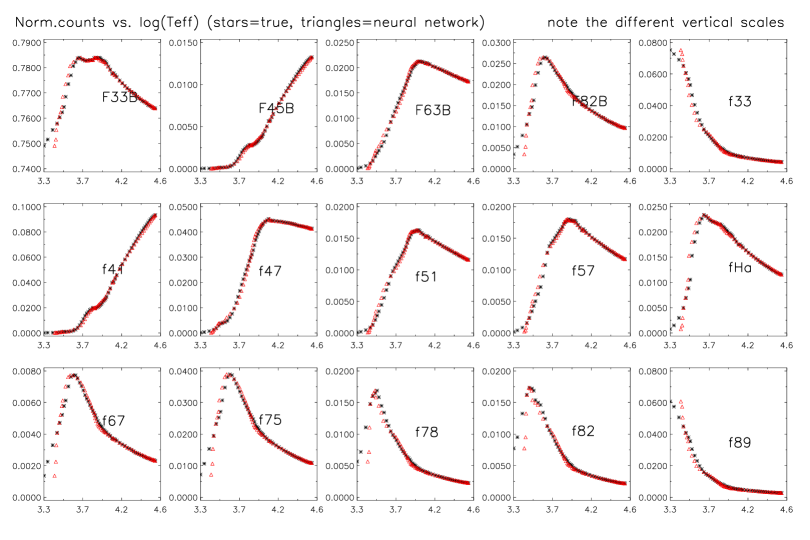
Figure 4: Each panel shows show the photon counts in a filter varies as a function of log ${\rm T}_{\rm eff}$ for stars with $\log g$ = 4.0 and [Fe/H] = 0.0 and zero extinction. The filter system is the 1X BBP+MBP system, with each filter named according to the first two digit of its central wavelength in nm. The trailing ‘B’ denotes a broad band (BBP) filter. The photon counts are normalized, that is their sum across all filters for a star is the same for all stars. The stars show the simulated data (stellar spectra passed through the Gaia instrument model) and the triangles the neural network predictions.

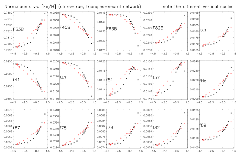
Figure 5: Same as Fig. 4, but now showing photon counts as a function of [Fe/H] for fixed ${\rm T}_{\rm eff}$ = 6000.

Examining Fig. 4 we see that the network has done very well in determining the ${\rm T}_{\rm eff}$ mapping. It manages to reproduce most of the small scale feature of the mappings. Only at the lowest temperatures does it have problems. This is due at least in part to the difficulty most regression models have at the boundaries of data sets, which arises because the regression is essentially only constrained on one side. In many of these one-dimensional cuts, the data to AP mapping is not single valued. The fact that the neural network can nonetheless produce the correct mapping shows that in this 15 dimensional data space the stellar data must lie on a lower dimensional manifold which does not show any serious degeneracies (for [Fe/H] and $\log g$ fixed). Fig. 5 shows the mapping as a function of metallicity keeping ${\rm T}_{\rm eff}$ and $\log g$ fixed. We straight away see that even though the true mapping is simpler, the neural network has more problems reproducing it. The reason for this can be seen when we compare the vertical (photon count) scale of the two plots: the variance in counts across the full range of [Fe/H] is much smaller than the count variance across the full range of ${\rm T}_{\rm eff}$. Putting it another way, [Fe/H] is a ‘weak’ AP compared to ${\rm T}_{\rm eff}$, in that varying [Fe/H] by X percent of its full range has a much smaller effect on the data (SED) than does varying ${\rm T}_{\rm eff}$ by the same amount. The effects of [Fe/H] are subtler and therefore harder to extract from the dominant effect of ${\rm T}_{\rm eff}$. This is compounded further by noise (which is small here) and the effects of the other parameters.

5 Areas currently under
investigation

The task of designing the classification system for Gaia, and for developing, testing and implementing the required algorithms, is the task of the Gaia Classification Working Group. A number of different tasks have been completed or have made some progress. These can be found in detail on the working group web site. Here I just provide a brief summary of the main tasks and provide the reference of the relevant working group document (things like ICAP-CBJ-013). These can be obtained from the ICAP web site or from Livelink.

• Design and implementation of the overall classification system. ICAP-CBJ-002/Bailer-Jones (2002), ICAP-CBJ-007, ICAP-CBJ-011.

• A ‘blind testing’ procedure to assess the performance of various photometric systems and classification algorithms for performing discrete classification and for estimating stellar parameters. ICAP-AB-003 (collation of results), ICAP-PW-001 (detailed analysis of MDM and neural network results for AP estimation), ICAP-CH-001 (analysis of various statistical algorithms for discrete classification and outlier detection).

• Minimum distance and perturbation methods. ICAP-VM-001.

• Identification and parametrization of unresolved binaries. ICAP-PW-003.

• Design of the Gaia photometric systems by direct optimization using evolutionary algorithms. ICAP-CBJ-013/Bailer-Jones (2004), GAIA-CBJ-016.

• The effect of CNO and $\alpha$ elements on the Gaia photometry. ICAP-GT-002.

• Stellar parameter uncertainty estimates using bootstrapping neural networks. ICAP-PW-004.

• Classification of QSOs and determination of their intrinsic parameters, including photometric redshift. Claeskens et al. (these proceedings).

Several articles in the present proceedings describe some of these and other classification issues in more detail. In particular see the contributions by Bailer-Jones, Carrasco et al., Claeskens et al., Girard & Soubiran, Maiz-Apellaniz, Malyuto, Picaud et al., Recio-Blanco et al., Willemsen et al. and Zwitter et al.

6 Issues and future work

Work on the classification system for Gaia is still in its early days. Given the heterogeneity of the Gaia data, plus the enormous range of objects and APs which it must deal with, classifying the Gaia data is not a simple task of applying some black box classifier to the entire data set. Some of the key issues which need to be addressed are as follows.

1. A proper handling of AP degeneracies. If degeneracies cannot be avoided in the photometric system (and they almost certainly cannot be), then we must at least identify where they occur. Because we know the forward mapping (data $\rightarrow$ APs) from stellar models, we can in principle determine this. This information could be used to perform a partition of the data space such that each partition is handled by a separate regression model, free of degeneracies.

2. Coping with ‘weak’ APs. Methods exist for boosting the sensitivity of a regression model to weak APs, e.g. increasing their contribution in the error minimization used to train the model (this is already used in our neural network models). However, other approaches need to be considered, such as iterative or hierarchical approaches in which first the strong APs are determined and then the weaker ones given our knowledge of the strong APs.

3. Dealing with systematic and correlated errors. This is related to the issue of ‘strong’ and ‘weak’ APs.

4. Training and regularization of models. While global models have some advantages over local ones, they are sensitive to the distribution (across APs) of the training data. This can introduce biases in the sense that it implicitly sets a prior probability on the APs of new objects.

5. Combining heterogeneous data. For sufficiently bright objects we have available two sets of photometric data (at different spatial resolutions), spectroscopic data and a parallax. It needs to be carefully considered how, from an algorithmic perspective, these data should best be combined to yield a self-consistent set of APs for a object. On the other hand, discrepancies could be important as they could indicate peculiar objects. Not all objects can be treated the same way. For example, the quality of the RVS data will vary enormously, and the good estimates of the data uncertainties which we can get from our instrument models should also be utilized.

6. Calibration. So far we have trained models and assessed performance mostly using synthetic data, as this is the only source of data at the required resolution and wavelength coverage (for simulating the Gaia photometry) covering the required wide range of APs. Determining physical parameters is the ultimate goal, so at some level stellar models and synthetic spectra must be used. But there will be limitations if we rely only on synthetic data for training models. One idea is to use a limited set of actual Gaia data of well-known stars to calibrate the classification models, for example by adjusting the training data. If insufficient well-known stars (with well determined APs) exist in Gaia’s catalogue, additional ground-based observations will be necessary to better characterize them in a homogeneous way. Such observing programs could and should start before the Gaia mission.

7. So far no attention has been paid to using morphological information, for example to perform star/galaxy discrimination. This will be partly the role of the onboard detection algorithms.

8. A number of issues have not yet been addressed, although work is starting on them. These include: galaxy classification; asteroid classification; classification of special types of stars (i.e. those for which we do not have reliable synthetic spectra); dealing with anomalous extinction. Finally, some kind of unsupervised classification, or internal classification scheme, should be investigated. Such approaches are independent of any physical models or pre-defined classification scheme and allow us to look for natural groupings within the data. This type of exploratory data analysis is an important complement for discovering new types of objects.

References

- (1) Bailer-Jones, C.A.L., 2002, Ap&SS, 280, 21
- (2) Bailer-Jones, C.A.L., 2004, A&A 419, 385
- (3) Hastie, T., Tibshirani, R., Friedman, J.H., 2001, The elements of statistical learning, Springer-Verlag