Cosmic microwave background polarization analysis

Abstract

With polarization of the cosmic microwave background (CMB) now detected, and confirmed by several independent experiments, the next goal is to characterise accurately its statistical properties. In these lecture notes we review the physical motivation for pursuing CMB polarization, and the basic statistical properties of the polarization fields. We then discuss some of the key aspects of the analysis of CMB polarization data, focusing on the additional complications that arise compared to temperature data due to the tensor character of the polarization field.

1 Introduction

The observed statistical properties of the temperature anisotropies in the cosmic microwave background (CMB) have played a key role in shaping our understanding of the large-scale properties of the Universe. The angular power spectrum of the anisotropies, quantifying the contribution to the variance of the anisotropies as a function of angular scale, has now been measured exquisitely over two decades of scale by the Wilkinson Microwave Anisotropy Probe (WMAP) satellite adc:bennett03 . A number of ground and balloon-borne experiments extend the power spectrum measurements by a further decade in scale but with somewhat less precision than has been attained on the larger scales (see adc:bond03 for a recent review). Current CMB data is remarkably consistent with predictions based on the passive evolution of density perturbations, with adiabatic initial conditions drawn from a Gaussian distribution with an almost-scale-invariant power spectrum, in a spatially-flat universe. Such primordial fluctuations, and the observed flat geometry of space, are natural outcomes of the simplest models of inflation in the early universe, e.g. adc:guth81 .

In addition to having angular variations in the total intensity, with r.m.s. $\sim 120\,\mu\mathrm{K}$, the CMB is also partially linearly polarized with r.m.s. $\sim 6\,\mu\mathrm{K}$. Polarization is generated by Thomson scattering of CMB photons around the time of recombination, once scattering becomes sufficiently rare to allow the development of anisotropies in the CMB intensity. Polarization is further generated at late times by re-scattering once the Universe reionizes. Despite being predicted shortly after the discovery of the CMB adc:rees68 , linear polarization wasn’t detected until 2002 by the Degree Angular Scale Interferometer (DASI) team adc:kovac02 . It has now been measured by two further groups adc:readhead04 ; adc:barkats05 , and also detected via its correlation with the temperature anisotropies in the first-year WMAP data adc:kogut03 . The direct measurements are currently much less precise than those for the temperature anisotropies, but they are fully consistent with predictions in models favoured by the temperature data. Future, precise measurements of CMB polarization will be very valuable, allowing accurate determination of several cosmological parameters that are almost degenerate in their effect on the temperature anisotropies adc:zaldarriaga97inf . The biggest winners will be the reionization history adc:zaldarriaga97reion , with the temperature–polarization correlation observed by WMAP already constraining the optical depth back to reionization to be $\sim 0.15$ adc:kogut03 , and constraints on any gravitational-wave background adc:seljak97 ; adc:kamionkowski97 and sub-dominant isocurvature modes adc:bucher01 .

As the accuracy and size of CMB datasets have grown, so have the demands on the techniques used to process the data. A standard set of compression and cleaning steps have emerged that ultimately distill $O(10^{10})$ time-ordered observations to several hundred power spectrum measurements, and only around 10 cosmological parameters and their errors (see e.g. adc:bond99 for a review.) Although the detail of some of these steps are instrument-specific, most analyses can be regarded as (approximate) variants on a small number of generic algorithms. Three of the most important steps are reviewed in detail elsewhere in this volume: for map making and power spectrum estimation see the contribution by Borrill; for (astrophysical) component separation and foreground removal see that by Delabrouille. Most of the steps in the analysis of CMB polarization data are straightforward generalisations of those for the temperature, but some new issues do arise mainly due to the tensorial nature of the polarization field. Furthermore, the small amplitude of the polarization signal demands that even more careful attention be paid to potential systematic effects in the analysis of polarization data than for the temperature anisotropies. Inevitably, this makes polarization data processing more instrument-specific and was the reason that the WMAP team did not release polarization maps with their first-year data.

The purpose of these lecture notes is to describe, in outline, the scientific motivation for pursuing CMB polarization, and discuss some of the key steps in the analysis of polarization data. We shall focus on those parts of the analysis that are complicated by the different geometric character of linear polarization compared to temperature anisotropies. To keep the discussion general, we will not have much to say on detailed instrument-specific parts of the analysis, although these are clearly crucial to the success of any given observation. We start in Sect. 2 with a discussion of the statistics of the CMB polarization fields and their representation in terms of orthonormal basis functions on the sphere. Section 3 reviews the basic physics of CMB polarization, and the current detections and best upper limits on CMB polarization are discussed in Sect. 4. What we have already learnt from current polarization measurements, and what we may learn in the future, is described in Sect. 5. The analysis of polarization data is then treated in Sect. 6, where discussions of map-making, astrophysical component separation, $E$- and $B$-mode separation, power spectrum estimation and non-Gaussian lensing issues can be found.

2 Statistics of CMB Polarization

The polarization on the sky along some line of sight $\hat{\vec{n}}$ is conveniently described in terms of Stokes specific brightness parameters $I(\hat{\vec{n}})$, $Q(\hat{\vec{n}})$, $U(\hat{\vec{n}})$ and $V(\hat{\vec{n}})$. For the CMB the total intensity $I(\hat{\vec{n}})$ has a Planck spectrum along any line of sight, but with angular temperature variations $\varDelta T(\hat{\vec{n}})$ at the $10^{-5}$ level on a 2.725-K background. In linear theory the anisotropic contribution to $I(\hat{\vec{n}})$ is thus proportional to $\varDelta T(\hat{\vec{n}})$ and has a spectrum given by the derivative of the Planck function (with respect to temperature). The parameters $Q$ and $U$ describe linear polarization, and inherit the spectrum of the anisotropic part of $I(\hat{\vec{n}})$ since CMB polarization is produced by frequency-independent Thomson scattering. The parameter $V$ describes circular polarization and is expected to vanish for the CMB.

For a line of sight $\hat{\vec{n}}$, the radiation is propagating along $-\hat{\vec{n}}$. If we introduce a pair of orthogonal directions in the surface of the sphere, and call these $x$ and $y$, such that $x$, $y$ and $-\hat{\vec{n}}$ form a right-handed basis, then the linear Stokes parameter $Q$ can be defined operationally as the difference between the intensities transmitted by perfect polarizers oriented along $x$ and $y$. Similarly, $U$ is the difference in intensities if the polarizers are rotated by $45^{\circ}$. We shall adopt the convention that in a spherical-polar coordinate system, the local $x$-axis is along the direction of decreasing polar angle $\theta$ (i.e. north) and the $y$-axis is along the direction of increasing azimuthal angle $\phi$ (i.e. east). This is in accordance with the IAU recommendations, but differs from e.g. adc:seljak97 and the latest version (1.2) of the HEALPix package. If the local $x$- and $y$-axes are rotated through an angle $\psi$ in a right-handed sense about the propagation direction, $Q$ and $U$ transform as

$$Q \rightarrow Q\cos 2\psi+U\sin 2\psi\;,$$

$$U \rightarrow U\cos 2\psi-Q\sin 2\psi\;.$$ (1)

These show that $Q$ and $U$ properly form the components (in an orthonormal basis) of a rank-2, symmetric trace-free tensor $\mathcal{P}^{ab}(\hat{\vec{n}})$ that is transverse to the line of sight:

$$\mathcal{P}^{ab}(\hat{\vec{n}})=\frac{1}{2}[Q(\hat{\vec{\theta}}\otimes\hat{\vec{\theta}}-\hat{\vec{\phi}}\otimes\hat{\vec{\phi}})-U(\hat{\vec{\theta}}\otimes\hat{\vec{\phi}}+\hat{\vec{\phi}}\otimes\hat{\vec{\theta}})]\;.$$ (2)

This linear polarization tensor is proportional to the correlation tensor (at zero lag) of the electric field components for the radiation propagating along $-\hat{\vec{n}}$.

Any two-dimensional tensor with the symmetries of $\mathcal{P}_{ab}$ can be derived from two scalar fields, denoted $P_{E}$ and $P_{B}$, via adc:seljak97 ; adc:kamionkowski97 :

$$\mathcal{P}_{ab}=\nabla_{\langle a}\nabla_{b\rangle}P_{E}+\epsilon^{c}{}_{\langle a}\nabla_{b\rangle}\nabla_{c}P_{B}\;,$$ (3)

where angle brackets denote the symmetric, trace-free part of the enclosed indices, $\nabla_{a}$ is the covariant derivative on the sphere, and $\epsilon_{ab}$ is the alternating tensor. The part derived from $P_{E}$ is the electric (or gradient) part and that from $P_{B}$ the magnetic (or curl) part of $\mathcal{P}_{ab}$. The divergence $\nabla^{a}\mathcal{P}_{ab}$ is a pure gradient if $P_{B}=0$, and a curl if $P_{E}=0$. The decomposition (3) is analogous to writing a vector field as a gradient and a divergence free vector, since in two dimensions the latter is always of the form ${\epsilon_{a}}^{b}\nabla_{b}\chi$. To gain some intuition for $E$ modes and $B$ modes, consider the case where $P_{E}$ and $P_{B}$ behave locally like a plane wave across a small patch of the sky (that can accurately be treated as flat). The electric and magnetic contributions to the polarization are depicted in Fig. 1. Quite generally, for a given potential $P$, the magnetic polarization $\mathcal{P}_{ab}^{B}\equiv\epsilon^{c}{}_{\langle a}\nabla_{b\rangle}\nabla_{c}P$ generated from $P$ is related to the electric polarization $\mathcal{P}^{E}_{ab}\equiv\nabla_{\langle a}\nabla_{b\rangle}P$ by $\mathcal{P}^{B}_{ab}={\epsilon^{c}}_{(a}\mathcal{P}^{E}_{b)c}$ which is a right-handed rotation of $\mathcal{P}^{E}_{ab}$ by $45^{\circ}$ about the line of sight.

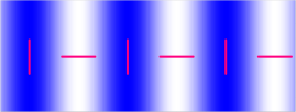
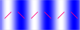
Figure 1: Polarization patterns for a pure-electric mode (left) and pure-magnetic mode (right) on a small patch of the sky for potentials that are locally Fourier modes. The shading denotes the amplitude of the potential. For the electric pattern the polarization is aligned with or perpendicular to the Fourier wavevector depending on the sign of the potential; for the magnetic pattern the polarization is at $45^{\circ}$.

The fields $P_{E}$ and $P_{B}$ are simple scalars that can be expanded in spherical harmonics with $l\geq 2$ as

$$P_{E}(\hat{\vec{n}})=\sum_{lm}\sqrt{\frac{(l-2)!}{(l+2)!}}E_{lm}Y_{lm}(\hat{\vec{n}})\;,\quad P_{B}(\hat{\vec{n}})=\sum_{lm}\sqrt{\frac{(l-2)!}{(l+2)!}}B_{lm}Y_{lm}(\hat{\vec{n}})\;.$$ (4)

(The normalisation is conventional.) The polarization tensor can then be written as

$$\mathcal{P}_{ab}(\hat{\vec{n}})=\frac{1}{\sqrt{2}}\sum_{lm}E_{lm}Y^{E}_{(lm)ab}+B_{lm}Y^{B}_{(lm)ab}\;,$$ (5)

where the trace-free, symmetric tensors

$$Y^{E}_{(lm)ab} \equiv \sqrt{\frac{2(l-2)!}{(l+2)!}}\nabla_{\langle a}\nabla_{b\rangle}Y_{lm}\;,$$

$$Y^{B}_{(lm)ab} \equiv \sqrt{\frac{2(l-2)!}{(l+2)!}}\epsilon^{c}{}_{(a}\nabla_{b)}\nabla_{c}Y_{lm}\;,$$ (6)

form orthonormal tensor bases for electric and magnetic polarization respectively. The electric and magnetic multipoles, $E_{lm}$ and $B_{lm}$, can be extracted directly from the polarization tensor by contraction with the appropriate tensor harmonic followed by integration over the sphere. For example,

$$E_{lm}=\sqrt{2}\int\mathcal{P}^{ab}Y^{E*}_{(lm)ab}\,\mathrm{d}\hat{\vec{n}}\;.$$ (7)

Methods of recovering $E$ and $B$ modes when observations cover only a limited part of the sky are discussed later in Sect. 6. Reality of $P_{E}$ and $P_{B}$ demands that $E_{lm}^{*}=(-1)^{m}E_{l\,-m}$, and similarly for $B_{lm}$.

We end this subsection by noting an alternative formalism for expressing symmetric, trace-free tensors on the sphere: the spin-weighted formalism adc:goldberg67 , first introduced to CMB physics in adc:seljak97 . The complex polarization $P\equiv Q+{\rm i}U$ is scaled by a phase factor $e^{-2{\rm i}\psi}$ under a right-handed rotation of the local $x$- and $y$-directions about the propagation direction, and so is defined to have spin -2. The appropriate basis functions for expanding functions of definite spin on the sphere are the spin-weighted spherical harmonics, ${}_{\pm 2}Y_{lm}(\hat{\vec{n}})$, which are related to the components of the tensor harmonics, $Y^{E}_{(lm)ab}$ and $Y^{B}_{(lm)ab}$, in a null diad:

$$Y^{E}_{(lm)ab} = \frac{1}{\sqrt{2}}({}_{-2}Y_{lm}m_{a}m_{b}+{}_{2}Y_{lm}m^{*}_{a}m^{*}_{b})\;,$$

$$Y^{B}_{(lm)ab} = \frac{1}{{\rm i}\sqrt{2}}({}_{-2}Y_{lm}m_{a}m_{b}-{}_{2}Y_{lm}m^{*}_{a}m^{*}_{b})\;.$$ (8)

Here the null (complex) vector $\vec{m}\equiv(\hat{\vec{\theta}}+{\rm i}\hat{\vec{\phi}})/\sqrt{2}$ satisfies $\vec{m}\cdot\vec{m}=0$ and $\vec{m}\cdot\vec{m}^{*}=1$. With $Q$ and $U$ expressed on the north–east basis of a spherical-polar coordinate system, the multipole expansion of the complex polarization is

$$(Q\pm{\rm i}U)(\hat{\vec{n}})=\sum_{lm}(E_{lm}\mp{\rm i}B_{lm}){}_{\mp 2}Y_{lm}(\hat{\vec{n}})\;.$$ (9)

The electric and magnetic multipoles can be extracted using the orthonormality of the spin-weighted harmonics, e.g.

$$E_{lm}\mp{\rm i}B_{lm}=\int(Q\pm{\rm i}U){}_{\mp 2}Y_{lm}^{*}\,\mathrm{d}\hat{\vec{n}}\;.$$ (10)

2.1 Polarization Power Spectra

The decomposition of the polarization field into electric and magnetic parts is invariant under rotations, and the electric and magnetic multipoles at fixed $l$ transform irreducibly under rotations, i.e. $E_{lm}\rightarrow D^{l}_{mm^{\prime}}E_{lm^{\prime}}$ where $D^{l}_{mm^{\prime}}$ are the Wigner functions (see e.g. adc:varshalovich ). Under the operation of parity, $(Q\pm{\rm i}U)(\hat{\vec{n}})\rightarrow(Q\mp{\rm i}U)(-\hat{\vec{n}})$ so that $E_{lm}\rightarrow(-1)^{l}E_{lm}$ (electric parity) while $B_{lm}\rightarrow(-1)^{l+1}B_{lm}$ (magnetic parity). These transformations ensure that the potential $P_{E}$ is a scalar under parity, $P_{E}(\hat{\vec{n}})\rightarrow P_{E}(-\hat{\vec{n}})$, but $P_{B}$ is a pseudo-scalar, $P_{B}(\hat{\vec{n}})\rightarrow-P_{B}(-\hat{\vec{n}})$. The temperature anisotropies $\varDelta T(\hat{\vec{n}})$ are a scalar function and so can be expanded in spherical harmonics in the usual way: $\varDelta T(\hat{\vec{n}})=\sum_{lm}T_{lm}Y_{lm}$. The multipoles $T_{lm}$ have electric parity.

In the absence of parity-violating interactions, the homogeneous and isotropic background universe on which cosmological perturbations are assumed to propagate can support an ensemble of fluctuations that is invariant under parity and rotations. What this means is that in the ensemble any fluctuation is just as likely as its parity-reversed, or rotated counterpart. The implication of this for the statistics of the CMB is that any expectation value must be preserved if we rotate or invert the fields involved. For the two-point statistics, this limits the non-zero correlations between the observable multipoles to

$$\langle T_{lm}T^{*}_{l^{\prime}m^{\prime}}\rangle=\delta_{ll^{\prime}}\delta_{mm^{\prime}}C_{l}^{T}\;,\quad \langle E_{lm}E^{*}_{l^{\prime}m^{\prime}}\rangle=\delta_{ll^{\prime}}\delta_{mm^{\prime}}C_{l}^{E}\;,$$

$$\langle B_{lm}B^{*}_{l^{\prime}m^{\prime}}\rangle=\delta_{ll^{\prime}}\delta_{mm^{\prime}}C_{l}^{B}\;,\quad \langle T_{lm}E^{*}_{l^{\prime}m^{\prime}}\rangle=\delta_{ll^{\prime}}\delta_{mm^{\prime}}C_{l}^{TE}\;.$$ (11)

For Gaussian fluctuations, such as those predicted by the simplest models of inflation, these power spectra $C_{l}^{T}$, $C_{l}^{E}$, $C_{l}^{B}$ and $C_{l}^{TE}$ contain all of the statistical information in the CMB. There have been several claims of violations of Gaussianity/rotational invariance in the one-year WMAP temperature data, e.g. adc:oliveira04 ; adc:vielva04 ; adc:copi04 ; adc:eriksen04 ; adc:hansen04 , but the issue of whether these are of primordial origin, or rather artifacts of the instrument or local Universe, is unresolved adc:schwarz04 . Example power spectra of the CMB observables for adiabatic density perturbations in a flat, $\Lambda$CDM model are shown in Fig. 2. The physics that gives rise to these spectra is reviewed briefly in Sect. 3.

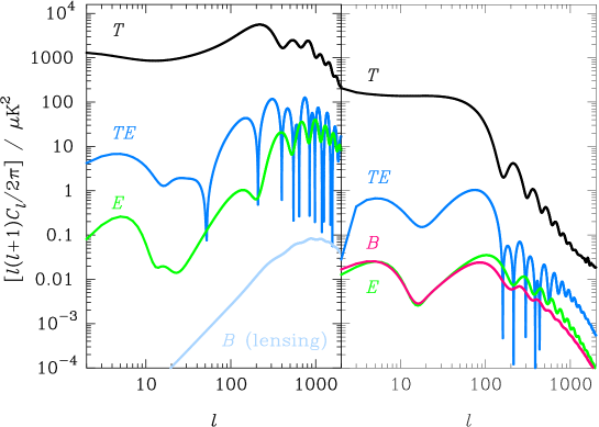
Figure 2: Power spectra produced by adiabatic scalar perturbations (left) and tensor perturbations (right) for a tensor-to-scalar ratio $r=0.38$.

It is also interesting to consider the two-point correlations between the Stokes parameters (and also the temperature anisotropies) in real space adc:coulson94 . For polarization, the correlation will be manifestly rotationally-invariant only if we work with Stokes parameters defined on a basis intrinsic to the two points, $\hat{\vec{n}}_{1}$ and $\hat{\vec{n}}_{2}$, under consideration. If we define the local $x$-direction by the geodesic connecting the two points, and denote the polarization on these bases by an overbar, the correlations are adc:kamionkowski97 ; adc:ng99 ; adc:chon04

$$\langle\bar{Q}(\hat{\vec{n}}_{1})\bar{Q}(\hat{\vec{n}}_{2})\rangle = \frac{1}{2}\sum_{l}\frac{2l+1}{4\pi}[C_{l}^{E}(d^{l}_{2\,2}+d^{l}_{2\,-2})(\beta)+C_{l}^{B}(d^{l}_{2\,2}-d^{l}_{2\,-2})(\beta)]\;,$$

$$\langle\bar{U}(\hat{\vec{n}}_{1})\bar{U}(\hat{\vec{n}}_{2})\rangle = \frac{1}{2}\sum_{l}\frac{2l+1}{4\pi}[C_{l}^{E}(d^{l}_{2\,2}-d^{l}_{2\,-2})(\beta)+C_{l}^{B}(d^{l}_{2\,2}+d^{l}_{2\,-2})(\beta)]\;,$$

$$\langle T(\hat{\vec{n}}_{1})\bar{Q}(\hat{\vec{n}}_{2})\rangle = \sum_{l}\frac{2l+1}{4\pi}C_{l}^{TE}d^{l}_{2\,0}(\beta)\;,$$

$$\langle T(\hat{\vec{n}}_{1})T(\hat{\vec{n}}_{2})\rangle = \sum_{l}\frac{2l+1}{4\pi}C_{l}^{T}d^{l}_{00}(\beta)\;,$$ (12)

where $\beta$ is the angle between the two points ($0\leq\beta\leq\pi$), and $d^{l}_{mn}(\beta)$ are the reduced Wigner functions. The correlations $\langle\bar{Q}\bar{U}\rangle$ and $\langle T\bar{U}\rangle$ vanish due to parity and rotational invariance. Examples of the non-zero polarization correlation functions are plotted in Fig. 3, along with a simulated Gaussian realisation of the temperature anisotropies on a flat patch of the sky with the correlated part of the polarization overlaid. As first noted in adc:coulson94 , the negative tail to the temperature–polarization correlation function on large scales is generic, arising from the infall of the photon–baryon plasma into potential wells around recombination, and gives a tangential pattern of correlated polarization around large-scale temperature hot spots. On smaller scales the sign of the cross-correlation oscillates. For adiabatic perturbations on scales smaller than $\sim 0.3^{\circ}$, the cross-correlation is positive and this gives rise to the tangential polarization pattern around small-scale cold spots that can be seen in Fig. 3.

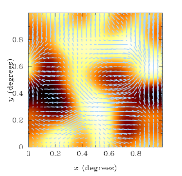
Figure 3: Polarization correlation functions for adiabatic density perturbations (left). The right-hand plot overlays a simulation of the correlated part of the polarization on the CMB temperature anisotropies.

Cosmic Variance

Since for Gaussian CMB fluctuations all cosmological information is encoded in the various power spectra, the precision with which the CMB can constrain cosmology is determined, in part, by the accuracy to which these spectra can be determined. In the absence of instrumental noise, and with full sky coverage, cosmic variance provides a fundamental limit to this accuracy. Cosmic variance arises from having a single realisation of a non-ergodic process (the sphere is compact) from which to estimate the power spectra. In this case, the obvious estimators of the power spectra, e.g.

$$\hat{C}_{l}^{E}=\frac{1}{2l+1}\sum_{m}|E_{lm}|^{2}\;,$$ (13)

are optimal in that they have the minimum variance of all unbiased estimators. At each $l$ we have only $2l+1$ independent real numbers from which to estimate a variance, so the cosmic variance in our estimator $\hat{C}_{l}^{E}$ for Gaussian fields is

$$\mathrm{var}(\hat{C}_{l}^{E})=\frac{2}{2l+1}(C_{l}^{E})^{2}\;.$$ (14)

Equivalent results apply to the two other auto-spectra $C_{l}^{T}$ and $C_{l}^{B}$. For the cross-spectrum, the cosmic variance is only slightly more complicated adc:kamionkowski97 ; adc:zaldarriaga97stats :

$$\mathrm{var}(\hat{C}_{l}^{TE})=\frac{1}{2l+1}\left[(C_{l}^{TE})^{2}+C_{l}^{T}C_{l}^{E}\right]\;.$$ (15)

The second term arises from chance correlations in the single realisation that we have available, and would fundamentally limit the accuracy of searches for parity violations via e.g. the cross-correlation between the temperature anisotropies and magnetic polarization. Due to the presence of correlations between the temperature and the electric polarization, estimates of $C_{l}^{T}$ and $C_{l}^{E}$ have non-vanishing covariance, and each is also correlated with the estimator for $C_{l}^{TE}$:

$$\mathrm{cov}(\hat{C}_{l}^{T},\hat{C}_{l}^{E})=\frac{2}{2l+1}(C_{l}^{TE})^{2}\;,\qquad\mathrm{cov}(\hat{C}_{l}^{T/E},\hat{C}_{l}^{TE})=\frac{2}{2l+1}C_{l}^{T/E}C_{l}^{TE}\;.$$ (16)

Of course, in the realistic case of non-zero instrument noise and limited sky coverage the precision of power spectrum estimates falls short of the cosmic variance limit. The effect of only observing a fraction $f_{\mathrm{sky}}$ of the sky is not only to increase the variance adc:scott94 , but also to correlate estimates across $\varDelta l$ given roughly by the inverse linear size of the retained portion of the sky adc:hobson96 ; adc:tegmark96 . The increase in variance can be crudely accounted for by reducing the number of independent modes to $(2l+1)f_{\mathrm{sky}}$. For polarization, this mode-counting argument ignores the loss of ambiguous modes that cannot be properly classified as electric or magnetic with partial sky coverage (see Sect. 6). This effect is minimised for surveys covering large connected regions of the sky.

3 Physics of CMB Polarization

When the mean free path was small compared to the spatial scale (i.e. wavelength for a plane wave) of the perturbations, Thomson scattering kept the CMB radiation isotropic in the rest frame of the electron–baryon plasma. As protons and electrons started to recombine to form neutral hydrogen, the mean free path increased and anisotropies started to develop. Subsequent Thomson scattering of the quadrupole component of the anisotropy generated linear polarization; this was then preserved for the free-streaming CMB until the Universe was reionized by the ionizing radiation from the first non-linear structures. The photon visibility function – the probability that a photon last scattered around recombination as a function of cosmic time – peaks around $370\;\mathrm{kyr}$ after the big bang and has a width $\sim 115\;\mathrm{kyr}$ adc:spergel03 . Since polarization is only generated by scattering it provides a very clean probe of conditions around the time of recombination and reionization.

Consider unpolarized radiation with a temperature distribution $\varTheta(\vec{e})$, where $\vec{e}$ is the radiation propagation direction. If the radiation field possesses a quadrupole anisotropy $\varTheta_{2}(\vec{e})$, Thomson scattering generates linear polarization with a polarization tensor adc:hu97angmom ; adc:challinor00

$$\mathcal{P}_{ab}(\vec{e})=-\frac{1}{20}\mathrm{d}\tau\nabla_{\langle a}\nabla_{b\rangle}\varTheta_{2}\;,$$ (17)

where $\mathrm{d}\tau$ is the differential optical depth, and the covariant derivatives are in the surface $\vec{e}^{2}=1$. Polarization is only generated from the quaudrupole component of the incident radiation, and can be seen to be purely electric quadrupole in character. If the incident radiation is polarized, there is an additional contribution to the polarization produced due to the electric quadrupole of the incident polarization ($\varTheta_{2}$ should be replaced by $\varTheta_{2}-12P_{E,2}$ adc:hu97angmom ; adc:challinor00 ). For the CMB, the linear polarization we observe (at $\vec{x}=0$) along a line of sight $\hat{\vec{n}}$ is that produced at last scattering along the radiation direction $\vec{e}=-\hat{\vec{n}}$, but at a direction-dependent comoving position $\vec{x}=\varDelta\eta\hat{\vec{n}}$. (We are assuming the Universe is flat for simplicity, and $\varDelta\eta$ is the conformal time between last scattering and the present.) The character of the observed polarization thus depends on the spatial distribution of the polarization at last scattering which, in turn, depends on the type of perturbations (e.g. density or gravitational waves) we consider.

3.1 Density Perturbations

If we consider a single plane-wave density perturbation of comoving wavenumber $k$, the peculiar velocity $\vec{v}_{\mathrm{b}}$ of the electron–baryon plasma around recombination is in the direction of the wavevector $\hat{\vec{k}}$. Over the mean free time since the previous scattering, a temperature quadrupole

$$\varTheta_{2}(\vec{e})\sim-\ell_{p}T_{\mathrm{CMB}}\nabla_{\langle i}v_{\mathrm{b},j\rangle}e^{i}e^{j}\propto T_{\mathrm{CMB}}\ell_{p}kP_{2}(\hat{\vec{k}}\cdot\vec{e})$$ (18)

is produced to leading order in $\ell_{p}k$ where $\ell_{p}$ is the mean free path. The quadrupole is azimuthally symmetric about the wavevector, and Thomson scatters to generate linear polarization parallel to the projection of $\hat{\vec{k}}$ on the sky (see Fig. 4). The polarization tensor at last scattering has a spatial dependence $\exp({\rm i}\vec{k}\cdot\vec{x})$ appropriate to the plane wave, and this leads to a further modulation of the polarization observed today by $\exp({\rm i}\varDelta\eta\vec{k}\cdot\hat{\vec{n}})$. This modulation transfers polarization from the $l=2$ to higher multipoles (with most appreciable power appearing at $l=k\varDelta\eta$), but preserves the electric character of the polarization adc:seljak97 ; adc:kamionkowski97 . To see that this is reasonable, note that the modulated polarization field has its polarization direction either parallel or perpendicular to the direction in which the polarization amplitude is changing adc:hu97primer . Comparison with Fig. 1 shows that such a pattern is pure electric polarization. This important observation, that linear density perturbations do not produce magnetic polarization, can also be understood from the fact that the spatial distribution of $\nabla_{\langle i}v_{\mathrm{b},j\rangle}$ is curl-free adc:challinor00 .

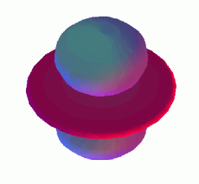
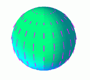
Figure 4: Generation of linear polarization by Thomson scattering for a single Fourier mode of the density perturbations, following the treatment of adc:hu97primer . The temperature anisotropies are azimuthally symmetric about the wavevector; the quadrupole part is shown on the left with cold lobes along the $\pm z$-directions. The linear polarization that is produced is then a pure $l=2$, $m=0$ electric polarization pattern locally (right). To get the observed polarization after free streaming from last scattering, the local polarization is modulated by the plane wave $\exp(i\vec{k}\cdot\hat{\vec{n}}\varDelta\eta)$.

An example of the polarization power spectra produced by adiabatic density perturbations is plotted in Fig. 2. They were computed with the Boltzmann code CAMB adc:lewis00 . The $E$-mode power peaks around $l\sim 1000$, corresponding to the angle subtended by the width of the visibility function at recombination. On larger scales the polarization probes the electron–baryon velocity at last scattering, as described above. Acoustic oscillations of the plasma prior to last scattering imprint an oscillatory structure on the angular power spectra of the CMB observables. Fourier modes of the photon density that are caught at the extrema of their oscillation at last scattering produce the peaks in the temperature-anisotropy power spectrum, but troughs in the polarization since $\vec{v}_{\mathrm{b}}$ then vanishes for such modes. Modes caught at either the extrema or the midpoint of their oscillation give zeroes in the temperature–polarization cross-correlation. Large-angle polarization from the last scattering surface is very small: the optimal wavelength for generating power at scale $l$ is $l/\varDelta\eta$, but this is too small to allow significant generation of quadrupole temperature anisotropies over a mean free path before last scattering. (Large-angle polarization is further suppressed since $\vec{v}_{\mathrm{b}}$ is small on super-Hubble scales.) The increase in polarization on large scales in Fig. 2 is due to reionization adc:zaldarriaga97reion . Re-scattering of the temperature quadrupole generates linear polarization peaking at multipoles roughly twice the ratio of the conformal look-back time to reionization to the conformal time elapsed between recombination and reionization. The amplitude of the polarization produced at reionization is proportional to the number of photons that scatter (i.e. the optical depth to reionization, taken to be $\tau=0.15$ in Fig. 2).

Although linear density perturbations do not produce $B$-mode polarization, this is produced by a number of second-order effects. The most notable is weak gravitational lensing by large-scale structure adc:zaldarriaga98lens , which effectively re-maps the polarization on the sky according to the lensing deflection field. This can distort a curl-free pattern into one with curl and so generate magnetic polarization. The power spectrum of this effect is also included in Fig. 2. On large scales the spectrum is almost white with $C_{l}^{B}\sim(1.3\,\mathrm{nK})^{2}$. The lens-induced $B$-mode spectrum peaks at $l\sim 1000$ corresponding to the peak in $C_{l}^{E}$.

3.2 Gravitational Waves

A stochastic background of gravitational waves, as predicted in all inflationary models, can also influence the CMB. Locally, a gravitational wave causes a quadrupole anisotropy in the expansion of space, so photons arriving at a scatterer from different lines of sight will suffer different redshifts since their previous scattering event. The longest wavelength gravitational waves are geometrically most efficient at generating a quadrupole moment. For wavelengths long compared to the mean free path, the quadrupole moment $\varTheta_{2}(\vec{e})\propto-\ell_{p}T_{\mathrm{CMB}}\dot{h}_{ij}e^{i}e^{j}/2$, where $h_{ij}$ is the transverse, trace-free perturbation to the Robertson–Walker metric,

$$\mathrm{d}s^{2}=a^{2}(\eta)[\mathrm{d}\eta^{2}-(\delta_{ij}+h_{ij})\mathrm{d}x^{i}\mathrm{d}x^{j}]\;,$$ (19)

and an overdot denotes differentiation with respect to proper time. However, the shear of the gravitational wave $\dot{h}_{ij}$ is zero for wavelengths well outside the horizon, and undergoes damped oscillation inside the horizon. It follows that the temperature quadrupole at last scattering is dominated by modes with wavelength of the order of the horizon size, and this sets the characteristic scale ($l\sim 100$) on which the polarization power spectra peak (see Fig. 2). Thomson scattering of the temperature quadrupole from gravitational waves generates a polarization tensor at last scattering $\mathcal{P}_{ab}\propto[\dot{h}_{ab}]^{\mathrm{TT}}$, i.e. proportional to the trace-free projection of the shear onto the sphere $\vec{e}^{2}=1$. For a single plane wave with wavevector along the $z$-axis, the quadrupole moment and local polarization from the plane wave have only $m=\pm 2$ modes (see Fig. 5 and adc:hu97angmom for further details). The observed polarization from a plane wave is further modulated by $\exp({\rm i}\varDelta\eta\vec{k}\cdot\hat{\vec{n}})$ in free-streaming from last scattering. Modulating the polarization in Fig. 5 gives a polarization pattern that locally looks electric along the lobes of the temperature quadrupole, and magnetic in between adc:hu97primer . It follows that both electric and magnetic polarization are generated by gravitational waves adc:seljak97 ; adc:kamionkowski97 , and with roughly equal powers adc:hu97angmom . The generation of $B$-mode polarization from gravitational waves can also be understood as a consequence of the non-vanishing (spatial) curl of the shear $\dot{h}_{ij}$ at last scattering adc:challinor00 .

The power spectra of the CMB observables from a scale-invariant background of gravitational waves is shown in Fig. 2. As for density perturbations, large-angle polarization is generated by reionization. The amplitude of any gravitational wave background is currently only weakly constrained by CMB observations. A recent analysis, combining CMB observations and data from the Sloan Digital Sky Survey (SDSS), constrained the tensor-to-scalar ratio $r$ – a measure of the ratio of the primordial power in gravitational waves to curvature (density) perturbations – to $r<0.36$ at 95% confidence in a seven-parameter flat model. This is similar to the value adopted in Fig. 2, and shows that the gravitational wave contribution to the temperature anisotropies and electric polarization is sub-dominant.

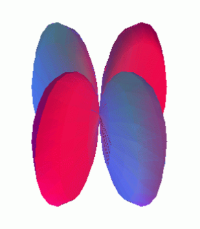
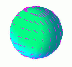
Figure 5: As in Fig. 4 but for a Fourier mode of the gravitational wave perturbations. The quadrupole part of the temperature anisotropy now has $m=\pm 2$ modes (left); the hot lobes correspond to the directions in which space is locally being contracted by the wave. The linear polarization produced by Thomson scattering (right) is again electric and quadrupole in character at the last scattering surface. Unlike density perturbations, magnetic polarization is now generated by free streaming since the polarization field modulated by the plane wave has a non-zero curl.

4 Current Status of CMB Polarization Measurements

The first detection of polarization of the CMB was announced in September 2002 adc:kovac02 . The measurements were made with DASI, a compact interferometric array operating at 30 GHz, deployed at the South Pole. The DASI team have now analysed three years of data; they report a detection of $E$-mode polarization at high significance ($6.3\sigma$) and at a level perfectly consistent with predictions based on temperature-anisotropy data adc:leitch04 . The only other reported direct detections to date are from the Cosmic Anisotropy Polarization MAPper (CAPMAP; adc:barkats05 ), a heterodyne correlation polarimeter operating at $90\,\mathrm{GHz}$ from New Jersey, and from the Cosmic Background Imager (CBI; adc:readhead04 ), an interferometer operating in the range 26–$36\,\mathrm{GHz}$ from Chile. The results on $C_{l}^{E}$ from maximum-likelihood power spectrum analyses by the DASI, CBI and CAPMAP teams are shown in Fig. 6, along with the prediction based on the best-fit to all the first-year WMAP data. Although the data are very noisy and broad-band (due to the limited sky coverage), the agreement with the prediction is striking. In addition, the $TE$ cross-correlation has been measured with good precision by WMAP adc:kogut03 , and has also been detected by DASI (see Fig. 6).

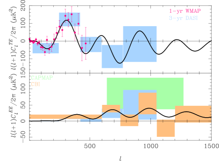
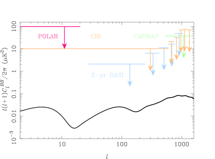
Figure 6: Current polarization detections and best upper limits (as of January 2005). The top plot shows $C_{l}^{TE}$ measurements (top) and $C_{l}^{E}$ (bottom). The points with 1-$\sigma$ errors are from the first one-year data release from WMAP. The error boxes are the flat band-power results from DASI, CBI and CAPMAP data, centred on the maximum-likelihood band power and spanning the 68-per cent intervals. The solid lines are the predicted power from the best-fit model to all the WMAP data. The bottom plot shows the upper limits on $C_{l}^{B}$ from DASI, CBI, CAPMAP and POLAR. The solid line assumes a tensor-to-scalar ratio $r=0.38$.

The $B$-mode polarization of the CMB is currently subject only to weak upper limits. The best limit on large scales, $l\sim 10$, is from the POLAR experiment adc:keating01 , while the best limits on smaller scales are from DASI adc:leitch04 . These (95%) upper limits are shown in Fig. 6, along with the predicted $B$-mode spectrum in a model with tensor-to-scalar ratio $r=0.38$, close to the current 95% limit from temperature anisotropies and SDSS adc:seljak04 . Current direct constraints on the amplitude of gravitational waves from $B$-mode data are clearly much weaker than this. Furthermore, upper limits on the $B$-mode power on small scales are at least two orders of magnitude above the level expected from gravitational lensing.

5 What do we learn from CMB polarization?

Electric polarization primarily traces the velocity of the electron–baryon plasma at recombination due to density perturbations. It thus provides complementary information to the temperature anisotropies which are sourced mainly by the photon density variations at last scattering on sub-degree scales. Polarization observations can thus be expected to bring significant improvements on some of the ‘acoustic’ cosmological parameters adc:zaldarriaga97inf , such as the physical density of baryons and cold dark matter, although current polarization data is not yet of sufficient quality relative to the temperature data to see this effect adc:readhead04 . Furthermore, the relative phase of the acoustic peaks in the temperature and electric-polarization power spectra (and the cross-correlation) can be used for a largely model-independent test of the physics of acoustic oscillations. For both adiabatic and isocurvature perturbations the acoustic peaks in $C_{l}^{T}$ and $C_{l}^{E}$ should be in antiphase. (Admixtures of these perturbations can, however, partially destroy this coherence.) A recent analysis by the CBI team adc:readhead04 found the phase of the oscillations in the $E$-mode spectrum to be fully consistent with expectations for adiabatic models. The spectrum $C_{l}^{TE}$ from the one-year WMAP data adc:kogut03 has also been used to improve constraints on the amplitude of any isocurvature fluctuations, e.g. adc:peiris03 ; adc:gordon03 ; adc:bucher04 .

Polarization on scales of tens of degrees ($l<10$) can be used to probe reionization. Significantly, it breaks the degeneracy between the amplitude of density perturbations, $A_{\mathrm{s}}$, and the optical depth to reionization, $\tau$, that leaves only $A_{\mathrm{s}}e^{-2\tau}$ well-determined from the temperature anisotropies. (The power spectra of the CMB observables are reduced by $e^{-2\tau}$ on scales corresponding to Fourier modes that are sub-horizon at reionization.) The one-year WMAP measurement of $C_{l}^{TE}$ shows a significant excess power on large scales that is attributed to early reionization ($11<z_{\mathrm{re}}<30$) giving a significant optical depth $\tau=0.17\pm 0.04$ (68% interval) adc:kogut03 . The amplitude of curvature (density) perturbations (at $0.05\,\mathrm{Mpc}$) is then constrained to $A_{\mathrm{s}}=(2.7\pm 0.3)\times 10^{-9}$ from the CMB alone adc:spergel03 . Looking further ahead, the fine details of the large-angle polarization power can, in principle, distinguish different ionization histories with the same optical depth, although this is hampered by the large cosmic variance at low $l$ adc:holder03 ; adc:hu03reion .

Perhaps the greatest ambition for CMB polarization observations is the detection of the $B$-mode signal from gravitational waves. Although gravitational waves do generate temperature anisotropies and electric polarization, they do so only on large scales where the cosmic variance of the dominant density perturbations is large. Indeed, a perfect temperature-anisotropy experiment can only detect $r>0.07$, even assuming all other parameters are known. Supplementing the temperature anisotropies with electric polarization makes only a modest further improvement: $r>0.02$. Although the current upper limit on $r$ from $B$-mode polarization is much weaker than that inferred from the CMB temperature anisotropies (see Fig. 6), the former route ultimately has the potential to probe much lower values as thermal noise levels improve. Assuming that astrophysical foregrounds can be removed adequately, the ultimate limit to a detection of the gravitational wave signal is set by the $B$-modes generated by gravitational lensing adc:knox02 ; adc:kesden02 ; adc:seljak04lens .

A detection of a stochastic background of gravitational waves would have significant implications for fundamental physics. In inflation models, the power produced in gravitational waves as a function of wavelength is a direct measure of the expansion rate of the Universe at the time that wavelength was stretched beyond the horizon. In slow-roll inflation in a potential $V$, the power in gravitational waves thus constrains the ‘energy scale of inflation’, $V^{1/4}$, via

$$V^{1/4}=3.33\times 10^{16}r^{1/4}(A_{\mathrm{s}}/2.3\times 10^{-9})^{1/4}\,\mathrm{GeV}\;.$$ (20)

The current 95% limit $r<0.36$ adc:seljak04 constrains $V^{1/4}<2.3\times 10^{16}\,\mathrm{GeV}$. By way of contrast, the recently-introduced cyclic model adc:steinhardt02 would produce negligible gravitational waves as the fluctuations are produced during a phase of very slow contraction adc:boyle04 . A detection of cosmological gravitational waves would effectively rule out such models. In addition to constraining the energy scale of inflation, measuring $r$ is important for constraining the shape of the inflaton potential. For the simplest models of slow-roll inflation, the observables $r$ and $n_{\mathrm{s}}$ (the spectral index of curvature perturbations) are both required to specify the first two derivatives of the inflaton potential. Without the tight limits on $r$ from future $B$-mode searches, constraints on inflation models will be largely degenerate along the direction of constant $n_{\mathrm{s}}$. The most recent constraints on $r$ and $n_{\mathrm{s}}$ from the CMB and galaxy surveys already rule out some popular models such as $V\propto\phi^{4}$ adc:seljak04 .

There are several other potential sources of $B$-mode polarization that could dominate over any signal of primordial gravitational waves from inflation. A sub-dominant background of cosmic strings – currently enjoying a resurgence of interest following the realisation that they are naturally produced in some models of brane inflation adc:jones02 – would provide a seed for gravitational waves (and vortical, or vector, modes) on the last scattering surface. Both give rise to $B$-mode polarization, and the resulting power spectrum is expected to peak on sub-degree scales adc:seljak97defect . It has been argued that a statistically-isotropic, but highly non-Gaussian, pattern of $B$-mode polarization with power peaking on small scales would be a smoking-gun signature for a background of cosmic strings adc:pogosian03 . In addition, primordial magnetic fields have several interesting effects on the CMB and its polarization, although the theory is still rather under-developed. The anisotropic stress of a stochastic field also excites gravitational waves and vector modes (e.g. adc:lewis04 ) leading to (non-Gaussian) $B$-mode polarization. Faraday rotation by either large-scale coherent adc:kosowsky96 ; adc:scannapieco97 or stochastic fields adc:kosowsky04 can also rotate electric polarization into magnetic. The hope is that these effects could be separated on the basis of their non-Gaussian statistical properties, and, in the case of Faraday rotation, by its frequency dependence.

Finally, we note that weak gravitational lensing effects on the CMB are a valuable source of additional cosmological information, most notably on the properties of dark energy and neutrino masses adc:hu02synergy . As we describe further in Sect. 6.6, CMB polarization is particularly useful here since intrinsically it has more power on small scales than the temperature and so is more sensitive to the small-scale power in the lensing deflection.

6 Polarization data analysis

The CMB polarization signal is small. Current measurements are consistent with the expected r.m.s. signal $\sim 6\,\mu\mathrm{K}$, which should be compared with the $\sim 120\,\mu\mathrm{K}$ r.m.s. of the temperature anisotropies. The low signal level requires high thermal sensitivity and demands exquisite control of systematic effects. The impact on the final science products of any systematics that cannot be designed out of the instrument must be carefully assessed (usually with a large number of simulations), and any that are found to be significant must be accounted for in the data analysis. As noted in the Introduction, this inevitably makes the analysis of polarization data more instrument-specific than for temperature-anisotropy experiments. Despite this, there are a number of common steps in the analysis pipeline of any polarization experiment: map-making from time-series data; astrophysical foreground removal; $E$-$B$ mode separation; power spectrum estimation; and parameter estimation. (Separation of $E$ and $B$ modes can also be performed statistically during the estimation of power spectra, and this has been the case for all analyses of real data to date.) In the following subsections we briefly summarise most of these key steps, but focus on $E$-$B$ separation and power spectrum estimation in particular. While the other steps are, of course, crucially important, the analysis methods employed there are relatively straightforward generalisations of those developed for the temperature anisotropies, for which excellent reviews already exist (see e.g. adc:bond01 ).

6.1 Modelling the polarimeter response

We begin by looking at how to model the response of a polarimeter, i.e. the relation between the observed data in the time domain to the fields on the sky. The most general (instantaneous) linear response of a polarimeter to the polarized sky brightness at each frequency is of the form

$$s\propto\int(\tilde{I}I+\tilde{Q}Q+\tilde{U}U-\tilde{V}V)\,\mathrm{d}\hat{\vec{n}}\;$$ (21)

Here, $I(\hat{\vec{n}},\nu)$, $Q(\hat{\vec{n}},\nu)$, $U(\hat{\vec{n}},\nu)$ and $V(\hat{\vec{n}},\nu)$ are the Stokes brightness parameters at frequency $\nu$, and the equivalent quantities with tildes refer to the instrument response. The latter parameters are determined by the instrument optics and receiver. They inherit a time-dependence from the scanning of the instrument on the sky – $\tilde{I}(\hat{\vec{n}},\nu)$ and $\tilde{V}(\hat{\vec{n}},\nu)$ rotate with the instrument as scalar functions and $\tilde{Q}(\hat{\vec{n}},\nu)$ and $\tilde{U}(\hat{\vec{n}},\nu)$ as components of a spin-2 function – but also from any modulation scheme employed to ameliorate the effects of low-frequency noise in the instrument. The signal contribution to the data is given by further integrating (21) over the spectral response of the instrument.

A useful idealisation is an instrument with ideal optics and receiver, and a narrow spectral bandpass. For a dual-polarization system, such as a pair of polarization-sensitive bolometers on the high-frequency instrument of the Planck satellite, the beam patterns on the sky for the two polarization modes should have field directions that are orthogonal and constant, and the amplitude of the response should be azimuthally symmetric. In the case of the bolometric system, the ideal instrument response is then fully determined by $\tilde{I}(\hat{\vec{n}})$, which is a function of $\theta$ only. The response to circular polarization vanishes and $\tilde{Q}\pm{\rm i}\tilde{U}=-\tilde{I}(\theta)\mathrm{e}^{\pm 2i\phi}$ for the $y$-polarization, and minus this for the $x$-polarization. If we now rotate the instrument so the optic axis is along the direction $\hat{\vec{n}}$, and the local $y$-polarization direction is at an angle $\psi$ to the $\phi$-direction there, the signal received in the $y$-polarization simplifies to adc:challinor00convolve

$$\int(\tilde{I}I+\tilde{Q}Q+\tilde{U}U-\tilde{V}V)\,\mathrm{d}\hat{\vec{n}}=I_{\mathrm{s}}(\hat{\vec{n}})-Q_{\mathrm{s}}(\hat{\vec{n}})\cos 2\psi+U_{\mathrm{s}}(\hat{\vec{n}})\sin 2\psi\;,$$ (22)

where the beam-smoothed fields are

$$I_{\mathrm{s}}(\hat{\vec{n}}) = \sum_{lm}W_{l}T_{lm}Y_{lm}(\hat{\vec{n}})\;,$$ (23)

$$(Q_{\mathrm{s}}\pm{\rm i}U_{\mathrm{s}})(\hat{\vec{n}}) = \sum_{lm}{}_{2}W_{l}(E\mp{\rm i}B)_{lm}{}_{\mp 2}Y_{lm}(\hat{\vec{n}})\;.$$ (24)

Here, the $W_{l}$ is proportional to the $m=0$ multipoles of $\tilde{I}(\theta)$ and ${}_{2}W_{l}$ to the $m=2$ electric multipoles of $\tilde{Q}\pm{\rm i}\tilde{U}$. For a Gaussian beam of dispersion $\sigma\ll 1$, we have beam functions

$$W_{l}\approx e^{-l(l+1)\sigma^{2}/2}\quad\mbox{and}\quad{}_{2}W_{l}\approx e^{-[l(l+1)-4]\sigma^{2}/2}\;.$$ (25)

For $l\gg 1$ the polarized and total intensity beam functions are very nearly equal. The form of (22) is equivalent to a point sampling of the smoothed fields along the optic axis with a polarizer in orientation $\psi$. The signal in the $x$-polarization is got by replacing $\psi$ by $\psi-\pi/2$. The generalisation of (22) to other ideal polarimeters is straightforward: in each case the signal remains a linear combination of the beam-smoothed fields.

6.2 Polarized map making

The aim of map-making is two-fold: (i) to produce pixelised images of the temperature and polarization fields on the sky from the observed data; and (ii) to compress the time-stream data to a more manageable size, while preserving as much of the cosmological information present as possible. We shall only consider the ideal instrument model described above; for a case study of some of the real-world problems that must be solved in the map-making process for total-intensity data see adc:stompor02 . For the ideal model, the signal contribution to the data is linear in the beam-smoothed fields. Instrument noise is assumed additive, in which case our simple model for the data from the $i$th detector at time $t$ becomes

$$d^{i}_{t}=A^{i}_{tp}(I_{\mathrm{s},p}-Q_{\mathrm{s},p}\cos 2\psi^{i}_{t}+U_{\mathrm{s},p}\sin 2\psi^{i}_{t})+n_{t}^{i}\;.$$ (26)

Here, $A^{i}_{tp}$ is the detector pointing matrix and is unity if the beam centre of detector $i$ points towards pixel $p$ at time $t$, and is zero otherwise. The $i$th detector at time $t$ is sensitive to polarization along a direction at angle $\psi^{i}_{t}$ to the $\phi$-direction on the sky, and has instrument noise $n^{i}_{t}$. We assume that all detectors have the same narrow spectral bandpass, and the same angular resolution, so that we can combine the signals of all detectors into a single vector $\vec{d}$ and the instrument noise into $\vec{n}$. We attempt to reconstruct the pixelised beam-smoothed fields, which we represent by the vector $\vec{s}$, by a regularised inversion of $\vec{d}=\mathsf{A}\vec{s}+\vec{n}$, where the $(it)p$ element of $\mathsf{A}$ is $A^{i}_{tp}$.

If the noise is Gaussian, with known covariance $\langle\vec{n}\vec{n}^{T}\rangle=\mathsf{N}$, the maximum-likelihood solution,

$$\hat{\vec{s}}=(\mathsf{A}^{T}\mathsf{N}^{-1}\mathsf{A})^{-1}\mathsf{A}^{T}\mathsf{N}^{-1}\vec{d}\;,$$ (27)

is optimal in the sense of being the minimum-variance unbiased estimate. The covariance of the errors is $\langle(\hat{\vec{s}}-\vec{s})(\hat{\vec{s}}-\vec{s})^{T}\rangle=(\mathsf{A}^{T}\mathsf{N}^{-1}\mathsf{A})^{-1}$. If the CMB fields are Gaussian, the maximum-likelihood map contains all of the cosmological information present in the time-stream data. In the language of statistics, the maximum-likelihood map is a sufficient statistic for parameter estimation, i.e. the data $\vec{d}$ only enters the posterior probability of the chosen (cosmological) parameters $\vec{\alpha}$ given the data, $\mathrm{Pr}(\vec{\alpha}|\vec{d})$, through $\hat{\vec{s}}$. Forming the maximum-likelihood map can thus also be viewed as lossless compression of the time-stream data. The question of the feasibility of computing the maximum-likelihood map is discussed in discussed in detail elsewhere in this volume by Borrill. Here we make just a few general remarks.

• Any matrix can be used in place of the noise covariance matrix $\mathsf{N}$ in (27) and the solution is still unbiased. However, if the matrix used does not properly capture the noise correlations described by off-diagonal elements of $\mathsf{N}$, the resulting maps will have correlations along the scan directions (‘stripes’).

• Brute-force evaluation of $\hat{\vec{s}}$ is prohibitive for large datasets so approximate methods must be used. For stationary noise, $\mathsf{N}$ is circulant and can be applied efficiently in the Fourier domain. Furthermore, direct inversion of $\mathsf{A}^{T}\mathsf{N}^{-1}\mathsf{A}$ can be avoided by solving $\mathsf{A}^{T}\mathsf{N}^{-1}\mathsf{A}\hat{\vec{s}}=\mathsf{A}^{T}\mathsf{N}^{-1}\vec{d}$ with iterative techniques.

• For stationary noise, the power spectrum (the diagonal elements of $\mathsf{N}$ in Fourier space) can be estimated from the data if it is not known a priori. Errors in the noise estimation increase the errors in the map.

• Maximum-likelihood map-making is easily generalised to include template fitting and marginalisation. For example, the unknown amplitude of some additive systematic effect whose ‘shape’ is known can be marginalised over during the map-making stage.

• Fast, instrument-specific alternatives to maximum-likelihood map-making have been proposed, e.g. the ‘destriping’ technique for Planck adc:delabrouille98 .

6.3 Astrophysical foreground removal

The dominant diffuse polarized foregrounds in the frequency range $20$–$400\,\mathrm{GHz}$ are expected to be Galactic synchrotron and vibrational (thermal) dust emission. Synchrotron radiation in a uniform magnetic field is linearly polarized. The polarization fraction depends on the energy spectrum of the electrons, but can plausibly be as high as 70%. Thermal dust emission will also be linearly polarized if non-spherical grains are aligned in a magnetic field. Any variation of the Galactic magnetic field along the line of sight will tend to depolarize the radiation reducing the polarization fraction. This depolarization tends to cancel the increased emission along the plane making the polarization dependence on Galactic latitude weaker than in total intensity. Synchrotron and dust emission can be expected to produce both electric and magnetic polarization in similar amounts adc:zaldarriaga01eb .

Synchrotron radiation is expected to be the dominant polarized foreground at frequencies below $\sim 100\,\mathrm{GHz}$. At the time of writing, the only well-surveyed part of the sky for which polarized data is available is within the Galactic plane, and then only at frequencies below 2.7 GHz (e.g. adc:duncan97 ). The only high-latitude observations available are very patchy adc:brouw76 , and most are not useful for assessing foreground contamination in clean regions of the sky that will likely be the target of future deep polarization observations. (But see adc:bernardi03 for a useful exception.) Analysis of the 2.7 GHz data of the Southern Galactic plane from adc:duncan97 gives $E$- and $B$-mode power spectra going as $l^{-1.5}$ adc:giardino02 , but care should be taken in extrapolating this to higher latitudes. A power law index of $-1.5$ is shallower than the large-angle polarization for both density perturbations and gravitational waves. Modelling at higher latitudes, based on total intensity observations (e.g. adc:giardino02 ), suggests that at frequencies around $100\,\mathrm{GHz}$, synchrotron emission will not be a major foreground for $E$-mode polarization, but that its removal will be essential for large-angle $B$-mode searches. We eagerly await the release of polarization maps from the two-year WMAP data; these should greatly improve our knowledge of high-latitude synchrotron polarization.

The power spectra from diffuse Galactic polarized dust emission have been measured recently at $353\,\mathrm{GHz}$ by the Archeops team adc:ponthieu05 over 20% of the sky. Extrapolating their measurements to $100\,\mathrm{GHz}$, they find for $3\leq l\leq 70$ that $(l+1)C_{l}^{E/B}/2\pi<0.2\,\mu\mathrm{K}^{2}$, excluding data with $5^{\circ}$ of the Galactic plane. Removal of the dust contamination is thus also likely to be necessary for future large-angle $B$-mode searches.

A variety of methods have been developed to remove diffuse foreground emission from CMB maps using multi-frequency data; see the contribution by Delabrouille in this volume for a review. Many of these were developed for total intensity data (temperature), but they generalise to polarization straightforwardly when applied directly to Stokes maps. Of these, some, such as Weiner filtering adc:bouchet99 , require knowledge of the frequency spectra of all the components present, and their angular power spectra. Others attempt to derive this information from the data by assuming statistical independence of the components adc:baccigalupi02 ; adc:delabrouille03 . Finally, linear techniques, based on template fitting adc:bennett03 , or internal spectral combinations that preserve the CMB signal while minimising the r.m.s. of the combined field, can also be applied very effectively to polarization data provided that the spectral properties of the contaminants do not vary too greatly over the survey area. The results of applying these techniques to simulated polarization data are very encouraging (e.g. adc:tucci04 ), but we must await further observations to assess the true extent to which foregrounds will compromise the scientific returns of CMB polarization surveys.

Extra-galactic radio sources are a significant polarized contaminant at small angular scales. They contribute equally to $E$- and $B$-mode power and, for Poisson-distributed sources, have white angular power spectra. An effective way to deal with these is simply to exclude pixels within an observing beam of known sources above some flux cut. Since the degree of polarization is typically rather low ($<10\%$), source contamination for $E$-mode polarization is relatively less troublesome than for temperature anisotropies. Having Stokes maps with a large number of excluded pixels does complicate the problem of separating $E$ and $B$ modes, and this is worse for low-resolution observations since the fraction of the area that is removed is then larger.

6.4 Map-level $E$ and $B$-mode separation

Separating the recovered polarization field into its electric and magnetic parts amounts to solving for the potentials $P_{E}$ and $P_{B}$ in (3). This can be done trivially if the observation covers the full sky by using the orthogonality of the electric and magnetic tensor harmonics to recover the multipoles $E_{lm}$ and $B_{lm}$ as in (7). However, problems arise for observations over only part of the sky since the decomposition $\mathcal{P}_{ab}=\nabla_{\langle a}\nabla_{b\rangle}P_{E}+\epsilon^{c}{}_{\langle a}\nabla_{b\rangle}\nabla_{c}P_{B}$ is then not unique adc:lewis02 ; adc:bunn03 . Even if fully-sky observations were available, we would want to remove certain regions (e.g. the Galactic plane) from the subsequent analysis, and this is most naturally done before the non-local decomposition into $E$ and $B$ modes.

To see how the ambiguity comes about, consider attempting to solve for $P_{E}$ and $P_{B}$ by recalling that the electric contribution to the divergence $\nabla^{b}\mathcal{P}_{ab}$ is curl-free and the magnetic part is divergence free, i.e.

$$2\nabla^{a}\nabla^{b}\mathcal{P}_{ab} = \nabla^{2}(\nabla^{2}+2)P_{E}\;,$$ (28)

$$-2\epsilon_{a}{}_{c}\nabla^{c}\nabla^{b}\mathcal{P}_{ab} = \nabla^{2}(\nabla^{2}+2)P_{B}\;.$$ (29)

Solving these equations over part of the sphere requires one to specify boundary data, namely the value of the potentials and their normal derivatives on the boundary adc:bunn03 . But this information is not known since it is the potentials that we are attempting to solve for. We can, of course, impose boundary conditions by force, in which case we should ensure that we do not produce spurious $E$ or $B$ modes, i.e. we should recover $P_{B}=0$ if there are no $B$-modes present. This will be true if we solve (28) and (29) with the boundary conditions that both the potentials and their gradients vanish on the boundary adc:lewis02 ; adc:bunn03 . In this manner, we obtain a unique solution for $P_{E}$ and $P_{B}$, but they are systematically wrong by $\varDelta P_{E}$ and $\varDelta P_{B}$ which are the unique solutions of $\nabla^{2}(\nabla^{2}+2)\varDelta P_{E}=0$ with $\varDelta P_{E}=P_{E}$ and $\nabla_{a}\varDelta P_{E}=\nabla_{a}P_{E}$ on the boundary (similar equations hold for $\varDelta P_{B}$). Reconstructing the polarization field from the recovered potentials, we see that this differs from the original field by $\varDelta\mathcal{P}_{ab}\equiv\nabla_{\langle a}\nabla_{b\rangle}\varDelta P_{E}+\epsilon^{c}{}_{\langle a}\nabla_{b\rangle}\nabla_{c}\varDelta P_{B}$. This part of the polarization field, which satisfies $\nabla^{a}\nabla^{b}\mathcal{P}_{ab}=0$ and $\epsilon_{a}{}_{c}\nabla^{c}\nabla^{b}\varDelta\mathcal{P}_{ab}=0$, constitutes the ambiguous part since it cannot be classified in terms of electric and magnetic modes. Some examples of these ambiguous modes are illustrated in adc:bunn03 ; adc:lewis03 . A useful vector analogy to keep in mind is that the ambiguous modes are like the electromagnetic fields of (static) charges and currents that are localised outside the observed region.

By excluding the ambiguous modes from subsequent analysis, we are throwing away some information. As we might expect, the ambiguous modes tend to be localised near the boundary, and a rough accounting of the fractional loss of modes as a function of scale is given by the ratio of the product of the boundary length and the coherence length to the observed area.

Practical methods for performing the separation described above are given in adc:lewis02 ; adc:bunn03 ; adc:lewis03 . The basic idea is to avoid differentiating the data by instead constructing tensor bases that can be used to project out the unambiguous $E$ and $B$ modes. Consider, for example, isolating magnetic polarization. If we construct a symmetric, trace-free tensor $W_{B\,ab}\equiv\sqrt{2}\epsilon^{c}{}_{(a}\nabla_{b)}\nabla_{c}W$ from a scalar field $W$ that vanishes, along with its gradient, on the boundary but is otherwise arbitrary. Contracting with the polarization tensor and integrating by parts gives adc:lewis02

$$\int W_{B}^{ab\ast}\mathcal{P}_{ab}\,\mathrm{d}\hat{\vec{n}}=-2\int W^{\ast}\epsilon^{b}{}_{c}\nabla^{c}\nabla^{a}\mathcal{P}_{ab}\,\mathrm{d}\hat{\vec{n}}\;,$$ (30)

where there are no boundary terms on account of the conditions imposed on $W$. It follows that the integral over the observed area is a non-local measure of the $B$-mode component. Similarly, the tensor $W_{E\,ab}\equiv\sqrt{2}\nabla_{\langle a}\nabla_{b\rangle}W$, with the same scalar field $W$, extracts a measure of the $E$-mode component. The construction of a complete set of such tensors can be performed in spherical-harmonic space adc:lewis02 ; adc:lewis03 (see also Sect. 6.5), or directly in pixel space adc:bunn03 . An orthonormal tensor basis can be constructed by taking the $W$ to be eigenfunctions of $\nabla^{2}(\nabla^{2}+2)$ (with the boundary conditions given above). Eigenfunctions with different eigenvalues are then orthogonal over the observed area, and the same is true of the tensors derived from them. Examples of $W_{B\,ab}$ basis functions for a circular patch of the sky are shown in Fig. 7. In this case the tensor bases can be constructed with $W$ an eigenfunction of $\partial/\partial_{\phi}$. For $m\geq 2$ exactly two $B$-modes are lost per $m$; for $m=$ only one is lost; and for $m=0$ none are lost. The basis functions in the figure are constructed to maximise the expected power in that mode.

Figure 7: Magnetic tensor basis functions $W_{B\,ab}$ for projecting onto pure magnetic-polarization modes for an azimuthally-symmetric sky patch of radius $10^{\circ}$ adc:lewis02 . Only $m=0$, 1 and 2 modes are shown. In each case only the three modes with the largest expected power are shown (with the left-most having greatest power).

The loss of information due to the ambiguous modes has interesting implications for survey design. For a fixed integration time, the ‘best’ strategy for measuring the variance of a Gaussian, statistically-isotropic field, in the limit of low signal-to-noise, is to survey only a small field since the error on the variance scales as the square-root of the survey area. (Of course, this is not a wise strategy as you may be unlucky and choose a field where the signal happens to be very low.) Applying this to searches for gravitational waves with $B$-mode polarization, the implication is that a small survey is best. However, the coherence length of the desired signal is around a degree so the loss of information to ambiguous modes becomes significant for small fields. The optimum field size on this basis turns out to be a circular patch with radius around $10^{\circ}$ adc:lewis02 . This argument ignores the effect of weak gravitational lensing. If we include the lens-induced $B$ modes as an additional Gaussian noise term, i.e. we make no attempt to clean out the lensing contribution as described in Sect. 6.6, the optimum size is increased further such that the contributions to the error on the variance from thermal noise and lensing sample variance are roughly equal.

We end this subsection by noting that coherent $E$-$B$ separation is not strictly necessary for constraining cosmology. A statistical separation can be attempted during power spectrum estimation (see Sect. 6.5), and for the optimal maximum-likelihood method this should be very effective. However, there are good reasons to perform a coherent, map-level separation as well. For example, visualising the $B$ modes will likely be a useful diagnostic of unknown systematic effects and foreground residuals.

6.5 Power spectrum estimation

The statistical properties of Gaussian random fields are fully specified by their power spectra. For this reason, power spectrum estimation is an important step in the analysis of CMB data. Ideally, this involves mapping out the likelihood $\mathrm{Pr}(\vec{s}|C_{l}^{R})$, where $\vec{s}$ are the observed CMB fields, as a function of the power spectra $C_{l}^{R}$ ($R=T$, $E$, $B$ or $TE$). In practice, what is normally done is to approximate the likelihood as a Gaussian function of the power spectra, in which case all of the information contained in the original CMB maps is distilled into the position of maximum likelihood, and the curvature of the likelihood there adc:bond98 . In this process, we achieve a very significant compression of the CMB maps into, at most, a few thousand maximum-likelihood $C_{l}$s, and their associated covariances. Even this programme is not achievable exactly for large data sets, so a number of faster techniques based on estimators have been suggested. Here, the idea is to construct (unbiased) estimators of the power spectra, and to use their covariances – or, better, their full sampling distributions adc:wandelt01 – to constrain cosmology. A particularly fast class of estimators are the heuristically-weighted, quadratic, or ‘pseudo-$C_{l}$’ estimators (e.g. adc:hivon02 ; adc:szapudi01 ). For an interesting critique of pseudo-$C_{l}$ and maximum-likelihood methods for temperature anisotropies, see adc:efstathiou04 . For polarization, both methods can be applied directly to maps of the Stokes parameters, in which case one must rely on a statistical separation of the $E$ and $B$ modes, or after map-level $E$-$B$ separation.

An important exception that demands a treatment beyond the power spectrum is the effect of weak gravitational lensing. Special techniques have been developed for this problem which allow reconstruction of the underlying Gaussian CMB and deflection fields (see Sect. 6.6). The power spectra of these reconstructed fields then contain all of the statistical (hence cosmological) information present in the non-Gaussian, lensed fields.

Maximum-likelihood methods

Maximum-likelihood methods, and the problems one faces in their practical implementation, are reviewed extensively elsewhere in this volume by Borrill. Here, we briefly summarise the technique. Maximum-likelihood methods have been used extensively in the analysis of real polarization data, e.g. from DASI adc:kovac02 and CBI adc:readhead04 .

For the direct analysis of Stokes maps (i.e. assuming no $E$-$B$ separation has been performed) we combine the observed Stokes parameters in a vector $\vec{s}=(I_{p},Q_{p},U_{p})^{T}$. The covariance matrix of this vector, $\mathsf{C}=\mathsf{S}+\mathsf{N}$, has contributions $\mathsf{S}$ from the signal and $\mathsf{N}$ from the noise. The former is given essentially by the temperature and polarization correlation functions (12), but with the following modifications: (i) the power spectra are multiplied by the appropriate product of the beam functions $W_{l}$ and ${}_{2}W_{l}$ to account for convolution with the instrument beam; and (ii) there are additional factors to account for the rotation of the Stokes parameters from the polar basis to the geodesic basis defined by the points $p$ and $p^{\prime}$. The noise contribution $\mathsf{N}$ includes the projection of the instrument noise onto the map, which will generally be modified by the foreground removal process, and an estimate of the covariance of any residual foreground errors. Both $\mathsf{S}$ and $\mathsf{N}$ have $(3N_{\mathrm{pix}})^{2}$ elements; $\mathsf{S}$ is dense in the pixel domain but is sparse in spherical-harmonic space, while $\mathsf{N}$ is typically sparse in the pixel domain. If map-level $E$-$B$ separation has already been performed, the data $\vec{s}$ can be taken as the unambiguous $E$ and $B$ modes, and these can be analysed independently (although the noise may correlate the errors in the estimated $E$- and $B$-mode power spectra). Assuming Gaussian signals and errors, the likelihood function is

$$\mathrm{Pr}(\vec{s}|C_{l}^{R})=\frac{1}{\sqrt{\mathrm{det}(2\pi\mathsf{C})}}\exp\left(-\vec{s}^{T}\mathsf{C}^{-1}\vec{s}/2\right)\,.$$ (31)

Maximising the likelihood is equivalent to maximising the posterior probability $\mathrm{Pr}(C_{l}^{R}|\vec{s})$ if a uniform prior on the power spectra, $C_{l}^{R}$, is adopted.

We now make some general remarks on this procedure.

• For full-sky coverage, and no noise, the log-likelihood is (up to an irrelevant constant)

  $$-2\ln\mathrm{Pr}(\vec{s}|C_{l}^{R}) = \sum_{l}(2l+1)\left[\frac{1}{\varDelta_{l}}(\hat{C}_{l}^{T}C_{l}^{E}+\hat{C}_{l}^{E}C_{l}^{T}-2\hat{C}_{l}^{TE}C_{l}^{TE})\right.$$ (32)

  $$\mbox{}\phantom{xxxxxxxxxxxxxxx}\left.+\ln\varDelta_{l}+\frac{\hat{C}_{l}^{B}}{C_{l}^{B}}+\ln C_{l}^{B}\right]\;,$$

  where $\varDelta_{l}\equiv C_{l}^{T}C_{l}^{E}-(C_{l}^{TE})^{2}$. The likelihood is approximately a Gaussian function of the $C_{l}^{R}$ at high $l$. The maximum-likelihood point coincides with the simple estimators e.g. $\hat{C}_{l}^{E}=\sum_{m}|E_{lm}|^{2}/(2l+1)$ at low $l$.

• Generally, the maximum of the likelihood can be located by solving $\partial\ln\mathrm{Pr}(\vec{s}|C_{l}^{R})/\partial C_{l}^{R}=0$, with e.g. the Newton–Raphson method. The data enters the gradient of the log-likelihood, and hence the maximum likelihood point, in the form $\vec{s}^{T}\mathsf{C}^{-1}(\partial\mathsf{S}/\partial C_{l}^{R})\mathsf{C}^{-1}\vec{s}$. This is proportional to the simple estimate $\hat{C}_{l}^{R}$, but with the spherical harmonic transforms taken only over the observed region, and with the data first weighted non-locally by $\mathsf{C}^{-1}$.

• Approximating the likelihood as Gaussian requires the computation of the curvature of the likelihood. At any $C_{l}^{R}$, the expectation value of the second derivatives of (minus) the log-likelihood there, under the assumption that these are the true power spectra, defines the Fisher matrix. The inverse of the Fisher matrix, evaluated at a smoothed version of the maximum likelihood power spectra, is often quoted as the error on the power spectra. For the ideal case, where the log-likelihood is given by (32), the inverse of the Fisher matrix has elements given by the cosmic variance formulae of Sect. 2.1.

• A brute-force implementation to locate the maximum likelihood, and evaluate the Fisher matrix, is not feasible for mega-pixel data sets. Both the operation count, $O(N_{\mathrm{pix}}^{3})$, and the storage requirements are prohibitive.

• Additional regularisation is required for small surveys since the problem is then degenerate if we attempt to solve for every multipole $l$. A common fix is to solve for bandpower amplitudes adc:bond98 . For narrow bands, approximating the $l(l+1)C_{l}$s as piecewise constant is common. As the polarization power spectra are steeper functions of $l$ than $C_{l}^{T}$, particularly on large scales, shaped bandpowers are often employed in polarization analyses (e.g. adc:kovac02 ).

Maximum-likelihood estimation is closely related to the optimal quadratic estimators adc:tegmark97 ; adc:tegmark01 . These take the form

$$\hat{C}_{l}^{R}=\frac{1}{2}\sum_{l^{\prime}R^{\prime}}F^{-1}_{(lR)(l^{\prime}R^{\prime})}\mathrm{trace}[(\vec{s}\vec{s}^{T}-\mathsf{N})\mathsf{C}^{-1}\partial\mathsf{S}/\partial C_{l^{\prime}}^{R^{\prime}}\mathsf{C}^{-1}],$$ (33)

where the Fisher matrix is $F_{(lR)(l^{\prime}R^{\prime})}\equiv\mathrm{trace}[\mathsf{C}^{-1}\partial\mathsf{S}/\partial C_{l}^{R}\mathsf{C}^{-1}\partial\mathsf{S}/\partial C_{l^{\prime}}^{R^{\prime}}]/2$. The quadratic estimator is unbiased for any (invertible) matrix $\mathsf{C}$, but the variance is minimised if $\mathsf{C}$ is truly the covariance of the data. Of course, this is not known a priori so we instead construct an approximation to $\mathsf{C}$ from some reasonable guess for the power spectra. It can be shown that iterating the quadratic estimator (i.e. constructing $\mathsf{C}$ for the next estimate from the current power spectrum estimates $\hat{C}_{l}^{R}$) is equivalent to performing a Newton–Raphson maximisation of the likelihood, with the curvature approximated by the Fisher matrix adc:bond98 . The optimal quadratic estimator has the same computational problems as maximum likelihood methods.

Heuristically-weighted, quadratic estimates

The computational complexity of the optimal quadratic estimator (33) arises from the non-local weighting of the data by the inverse covariance matrix $\mathsf{C}^{-1}$. Heuristically-weighted, quadratic methods adc:chon04 ; adc:wandelt01 ; adc:hivon02 ; adc:szapudi01 ; adc:hansen03 circumvent this problem by adopting a local weighting scheme. The use of fast-spherical transforms, as implemented in e.g. the HEALPIX package adc:gorski04 , reduce the operations count to $O(N_{\mathrm{pix}}^{3/2})$ which is fast enough to be used in high-volume simulations.

We shall concentrate here on the polarization auto-correlations only. Including the cross-correlation between temperature and polarization is straightforward adc:chon04 ; adc:hansen03 . Assuming we are analysing Stokes maps, we adopt a real weighting $w(\hat{\vec{n}})$ that is zero where we have no data. For the case of temperature anisotropies, weighting with the inverse noise variance on scales where the noise dominates the signal, and uniformly where the signal dominates, can be shown to be close to optimal adc:efstathiou04 . Care should be taken in generalising this reasoning to low-amplitude $B$-mode polarization because of the additional complication of $E$-$B$ mixing. We extract the electric and magnetic multipoles of the weighted polarization field with spherical transforms,

$$\tilde{E}_{lm}\pm{\rm i}\tilde{B}_{lm} \equiv \int w(\hat{\vec{n}})(Q\mp{\rm i}U)(\hat{\vec{n}}){}_{\pm 2}Y_{lm}^{*}(\hat{\vec{n}})\,\mathrm{d}\hat{\vec{n}}\;,$$ (34)

$$= \sum_{(lm)^{\prime}}{}_{\pm 2}I_{(lm)(lm)^{\prime}}(E_{(lm)^{\prime}}\pm{\rm i}B_{(lm)^{\prime}})\;,$$

where the Hermitian coupling matrices are

$${}_{\pm 2}I_{(lm)(lm)^{\prime}}\equiv\int w(\hat{\vec{n}}){}_{\pm 2}Y_{(lm)^{\prime}}(\hat{\vec{n}}){}_{\pm 2}Y_{lm}^{*}(\hat{\vec{n}})\,\mathrm{d}\hat{\vec{n}}\;,$$ (35)

and can be expressed in terms of the (scalar) multipoles, $w_{lm}$, of the weight function, and the Wigner $3j$ symbols adc:hansen03 . We have left the effect of smoothing by the instrument beam implicit in (34); the factors ${}_{2}W_{l}$ can be absorbed into the multipoles $E_{lm}$ and $B_{lm}$, and, later, ${}_{2}W_{l}^{2}$ into the power spectra $C_{l}^{E}$ and $C_{l}^{B}$. We compress the pseudo-multipoles into pseudo-$C_{l}$s according to

$$\tilde{C}_{l}^{E}\equiv\frac{1}{2l+1}\sum_{m}|\tilde{E}_{lm}|^{2}\quad,\quad\tilde{C}_{l}^{B}\equiv\frac{1}{2l+1}\sum_{m}|\tilde{B}_{lm}|^{2}\;.$$ (36)

These quantities are equivalent to the $\vec{s}^{T}\mathsf{C}^{-1}(\partial\mathsf{S}/\partial C_{l}^{R})\mathsf{C}^{-1}\vec{s}$ that appear in the optimal quadratic estimator (33) if we replace $\mathsf{C}^{-1}$ by heuristic weights.

$E$-$B$ mixing revisited

We make a brief aside to note the relation between the pseudo-multipoles and the issue of separating $E$ and $B$ modes with incomplete sky coverage. The pseudo-multipoles mix $E$ and $B$ modes according to

$$\tilde{E}_{lm} = \sum_{(lm)^{\prime}}\left({}_{+}I_{(lm)(lm)^{\prime}}E_{(lm)^{\prime}}+{\rm i}{}_{-}I_{(lm)(lm)^{\prime}}B_{(lm)^{\prime}}\right)\;,$$ (37)

$$\tilde{B}_{lm} = \sum_{(lm)^{\prime}}\left({}_{+}I_{(lm)(lm)^{\prime}}B_{(lm)^{\prime}}-{\rm i}{}_{-}I_{(lm)(lm)^{\prime}}E_{(lm)^{\prime}}\right)\;,$$ (38)

where we have defined the Hermitian ${}_{\pm}I_{(lm)(lm)^{\prime}}$ to be

$${}_{+}I_{(lm)(lm)^{\prime}} \equiv \frac{1}{2}({}_{+2}I_{(lm)(lm)^{\prime}}+{}_{-2}I_{(lm)(lm)^{\prime}})=\int wY^{E\,*}_{(lm)\,ab}Y^{E\,ab}_{(lm)^{\prime}}\,\mathrm{d}\hat{\vec{n}}\;,$$ (39)

$${}_{-}I_{(lm)(lm)^{\prime}} \equiv \frac{1}{2}({}_{+2}I_{(lm)(lm)^{\prime}}-{}_{-2}I_{lm(lm)^{\prime}})=-i\int wY^{E\,*}_{(lm)\,ab}Y^{B\,ab}_{(lm)^{\prime}}\,\mathrm{d}\hat{\vec{n}}\;.$$ (40)

The mixing matrix ${}_{-}I_{(lm)(lm)^{\prime}}$ controls the mixing of $E$ modes into $\tilde{B}_{lm}$, and vice versa. For the case of uniform weighting over the full sky, the mixing matrix vanishes and ${}_{+}I_{(lm)(lm)^{\prime}}\propto\delta_{ll^{\prime}}\delta_{mm^{\prime}}$. For partial sky coverage, if $w(\hat{\vec{n}})$ is unity inside the observed region but zero elsewhere, integrating by parts in (40) shows that ${}_{-}I_{(lm)(lm)^{\prime}}$ reduces to a line integral around the boundary adc:lewis02 :

$$i{}_{-}I_{(lm)(lm)^{\prime}}=\sqrt{\frac{2(l-2)!}{(l+2)!}}\oint\left(\nabla_{b}Y^{*}_{lm}Y^{B\,ab}_{(lm)^{\prime}}-Y^{*}_{lm}\nabla_{b}Y^{B\,ab}_{(lm)^{\prime}}\right)\,\mathrm{d}l_{a}\;.$$ (41)

If we contract the $\tilde{B}_{lm}$ with the multipoles $W^{*}_{lm}$ of any scalar function $W(\hat{\vec{n}})=\sum_{lm}W_{lm}Y_{lm}(\hat{\vec{n}})$, such that $W$ and $\nabla_{a}W$ vanish on the boundary of the observed region, we see that $\sum_{lm}W^{*}_{lm}{}_{-}I_{(lm)(lm)^{\prime}}=0$ and we will have projected out the $E$-mode contamination from the $\tilde{B}_{lm}$. Since the construction $\sum_{lm}W^{*}_{lm}\tilde{B}_{lm}$ is equivalent to integrating the contraction of $W_{B}^{ab\,*}=\sqrt{2}\epsilon^{c}{}_{(a}\nabla_{b)}\nabla_{c}W^{*}$ and $\mathcal{P}_{ab}$ over the observed region, isolating those functions in harmonic space that are orthogonal to the range of ${}_{-}I_{(lm)(lm)^{\prime}}$ is equivalent to finding elements of the tensor basis of the unambiguous $E$ and $B$ modes over the observed region (see Sect. 6.4). The harmonic-space method for $E$-$B$ separation developed in adc:lewis02 uses singular value techniques to project out the range of the mixing matrix ${}_{-}I_{(lm)(lm)^{\prime}}$.

For a more general weight function $w(\hat{\vec{n}})$, if we assume that it smoothly apodizes the edges of a connected region of linear dimension $\sim R$, the relative sizes of ${}_{-}I$ and ${}_{+}I$ at scale $l^{-1}$ are in the ratio $1/(lR)$ adc:challinor04 . It follows that the geometric effect of mode mixing is suppressed on scales small compared to the survey size.

Mean values of the pseudo-$C_{l}$s

Figure 8: Left: power spectra for $B$ (top) and $E$ (bottom; solid lines) compared to the mean pseudo-$C_{l}$s (dotted lines) and the recovered power spectra (dashed lines). Right: the bottom panel shows representative matrices $P_{ll^{\prime}}$ (solid lines) and $M_{ll^{\prime}}$ (dotted lines); the top panel shows the pseudo-inverses $\tilde{P}^{-1}_{ll^{\prime}}$ (solid lines) and $\tilde{M}^{-1}_{ll^{\prime}}$ (dotted lines). Note that $M_{ll^{\prime}}$ and $\tilde{M}^{-1}_{ll^{\prime}}$ have been multiplied by a factor of 100 for clarity. The weight function applied to the map is uniform inside a circle of $10^{\circ}$ radius, with cosine apodization out to $15^{\circ}$. To obtain the pseudo-inverses, a Gaussian apodization of $4^{\circ}$ HWHM is applied to the correlation functions.

Returning to the pseudo-$C_{l}$s, their mean values contain two contributions, one from the covariance of the instrument noise (and foreground residuals) and one from the CMB power spectra. The former can be estimated by using a large number of simulated observations: $\sim 10^{4}$ observations should give $\sim 1\%$ accuracy. The mean level in the simulations can then be subtracted from the observed $\tilde{C}_{l}$ to remove the noise bias in the mean. From now on we shall assume that the pseudo-$C_{l}$s have been corrected in this way. Alternatively, if only correlations between different instrument channels are used in the construction of the pseudo-$C_{l}s$, the noise bias will vanish if the noise is uncorrelated between channels adc:hinshaw03 . The means of the pseudo-$C_{l}$s are then linearly related to the true power spectra:

$$\langle\tilde{C}_{l}^{E}\rangle=\sum_{l^{\prime}}P_{ll^{\prime}}C_{l^{\prime}}^{E}+M_{ll^{\prime}}C_{l^{\prime}}^{B}\;,\qquad\langle\tilde{C}_{l}^{B}\rangle=\sum_{l^{\prime}}M_{ll^{\prime}}C_{l^{\prime}}^{E}+P_{ll^{\prime}}C_{l^{\prime}}^{B}\;.$$ (42)

Here, the matrices are $P_{ll^{\prime}}\equiv\sum_{mm^{\prime}}|{}_{+}I_{(lm)(lm)^{\prime}}|^{2}/(2l+1)$, with a similar expression for $M_{ll^{\prime}}$. They depend on the weight function $w(\hat{\vec{n}})$ only through the rotational invariant $w_{l}\equiv\sum_{m}|w_{lm}|^{2}/(2l+1)$, and can be expressed in terms of $3j$ symbols as

$$(P/M)_{ll^{\prime}}=\frac{2l^{\prime}+1}{8\pi}\sum_{L}(2L+1)w_{L}[1\pm(-1)^{l+l^{\prime}+L}]\left(\begin{array}[]{ccc}l&l^{\prime}&L\\ -2&2&0\end{array}\right)^{2}\;.$$ (43)

For uniform weighting over the full sky, only $w_{0}$ is non-zero and so $M_{ll^{\prime}}$ vanishes as it must (the $3j$ symbol forces $l=l^{\prime}$ and hence $l+l^{\prime}+L$ to be even). For weight functions that smoothly apodize observations over a region of linear size $\sim R$, the weight function is almost band-limited to $l_{\mathrm{max}}\sim 1/R$. In this case the $P_{ll^{\prime}}$ and $M_{ll^{\prime}}$ matrices are close to band diagonal, and, for spectra that are smooth on the scale of $R^{-1}$, the means of the pseudo-$C_{l}$s are approximately

$$\langle\tilde{C}_{l}^{E}\rangle\approx C_{l}^{E}\sum_{l^{\prime}}P_{ll^{\prime}}+C_{l}^{B}\sum_{l^{\prime}}M_{ll^{\prime}}\;,\qquad\langle\tilde{C}_{l}^{B}\rangle\approx C_{l}^{E}\sum_{l^{\prime}}M_{ll^{\prime}}+C_{l}^{B}\sum_{l^{\prime}}P_{ll^{\prime}}\;.$$ (44)

The relative size of the mixing of $E$- and $B$-mode power in the pseudo-$C_{l}$s is thus set by the ratio of the normalisations $\sum_{l^{\prime}}M_{ll^{\prime}}$ to $\sum_{l^{\prime}}P_{ll^{\prime}}$. For $l\gg 1/R$, it can be shown that adc:challinor04

$$\sum_{l^{\prime}}P_{ll^{\prime}} \approx \frac{1}{4\pi}\int w^{2}(\hat{\vec{n}})\,\mathrm{d}\hat{\vec{n}}\;,$$ (45)

$$\sum_{l^{\prime}}M_{ll^{\prime}} \approx \frac{1}{2\pi}\frac{1}{l(l+1)}\int(\nabla w)^{2}(\hat{\vec{n}})\,\mathrm{d}\hat{\vec{n}}\;,$$ (46)

so that mixing of power is suppressed by $1/(lR)^{2}$. Given that it is expected that $C_{l}^{E}\gg C_{l}^{B}$ on all scales, $\langle\tilde{C}_{l}^{E}\rangle$ is essentially a scaled version of the true spectrum, but this need not be the case for $\tilde{C}_{l}^{B}$. These ideas are illustrated in Fig. 8 which show typical rows of the matrices $P_{ll^{\prime}}$ and $M_{ll^{\prime}}$, and the mean pseudo-$C_{l}$s that they give rise to, for observations covering a circle of radius $15^{\circ}$ with the last $5^{\circ}$ apodized with a cosine function. The mean of $\tilde{C}_{l}^{E}$ is seen to be a scaled version of the true power spectrum except on large scales, but this is not the case for $\tilde{C}_{l}^{B}$.

‘Unbiased’ estimators

The pseudo-$C_{l}$s can be used directly for parameter estimation adc:wandelt01 , but it is often desirable to deconvolve the geometric effects of the weight function so we have unbiased estimates of the underlying power spectra. For example, for presentation purposes it is useful if we can plot the data in a form where they can be easily compared with true power spectra.

For observations covering a significant fraction of the sky, deconvolution is straightforward. The matrices $P_{ll^{\prime}}\pm M_{ll^{\prime}}$ will then be invertible and we can form unbiased estimates of the power spectra according to

$$\hat{C}_{l}^{E}\pm\hat{C}_{l}^{B}=\sum_{l^{\prime}}(P\pm M)^{-1}_{ll^{\prime}}(\tilde{C}_{l^{\prime}}^{E}\pm\tilde{C}_{l^{\prime}}^{B})\;.$$ (47)

An equivalent formulation of this approach can be made in terms of correlation functions adc:chon04 ; adc:szapudi01 . Consider estimating the correlation functions (11) by averaging over pairs of pixels separated by $\beta$, with pairs weighted by $w(\hat{\vec{n}}_{1})w(\hat{\vec{n}}_{2})$. It turns out that the data enters the estimators only through its pseudo-$C_{l}$s. The estimators $\hat{\xi}_{\pm}(\beta)$ for $\langle(\bar{Q}\mp{\rm i}\bar{U})(\hat{\vec{n}}_{1})(\bar{Q}+{\rm i}\bar{U})(\hat{\vec{n}}_{2})\rangle$, where $\hat{\vec{n}}_{1}\cdot\hat{\vec{n}}_{2}=\cos\beta$, can be expressed as adc:chon04

$$\hat{\xi}_{\pm}(\beta)=\frac{\sum_{l}(2l+1)(\tilde{C}_{l}^{E}\pm\tilde{C}_{l}^{B})d^{l}_{2\,\pm 2}(\beta)}{\sum_{l}w_{l}P_{l}(\cos\beta)}\;,$$ (48)

which also provides an efficient $O(N_{\mathrm{pix}}^{3/2})$ way of estimating the correlation functions. If enough sky is available to estimate the correlation functions for all $\beta$, then we can recover unbiased estimates of the power spectra by integral transforms. Using the orthogonality of the reduced Wigner functions, we have

$$\hat{C}^{E}_{l}\pm\hat{C}^{B}_{l}=2\pi\int_{-1}^{+1}\hat{\xi}_{\pm}(\beta)d^{l}_{2\,\pm 2}(\beta)\,\mathrm{d}\cos\beta\;.$$ (49)

The integration can be performed essentially exactly with Gauss–Legendre integration, and a significant feature of estimating the correlation functions via the pseudo-$C_{l}$s is that they can be evaluated for any $\beta$ up to the maximum pixel separation in the map. This avoids the need to re-sample the correlation functions onto the points required for the quadrature. This method has recently been applied to estimate the power spectra from the polarized channel of Archeops adc:ponthieu05 . Aside from discretisation issues, this correlation function method is equivalent to performing the direct inversion in (47).

For small surveys we will not have pixels separated by all angles $\leq 180^{\circ}$, in which case we cannot estimate the correlation functions for all $\beta$. The inversion in (49) is then not possible. This is equivalent to saying that the survey does not have the spectral resolution to perform the matrix inversions in (47). Various schemes can be adopted to regularise the inversion, such as the use of bandpowers adc:hivon02 . Alternatively, we can settle for pseudo-inverses $\tilde{P}^{-1}_{ll^{\prime}}$ and $\tilde{M}^{-1}_{ll^{\prime}}$, constructing estimators, e.g.

$$\hat{C}_{l}^{B}=\sum_{l^{\prime}}\tilde{P}^{-1}_{ll^{\prime}}\tilde{C}_{l^{\prime}}^{B}+\tilde{M}^{-1}_{ll^{\prime}}\tilde{C}_{l^{\prime}}^{E}\;,$$ (50)

that have a simpler relation to the true power spectra than do the pseudo-$C_{l}$s. One desirable property we might enforce on the pseudo-inverses is that $E$-$B$ mixing is removed in the mean, i.e. $\langle\hat{C}_{l}^{B}\rangle$ has no contribution from $C_{l}^{E}$. A convenient way to find such a pseudo-inverse is given in adc:chon04 , which builds on earlier work in the context of cosmic shear analysis adc:crittenden02 . We make use of the correlation functions estimates (48) in the angular range $(0,\beta_{\mathrm{max}})$, where $\beta_{\mathrm{max}}$ is the maximum separation of pixels in the Stokes maps. It is shown in adc:chon04 that the estimators $\hat{\xi}(\beta)\pm\hat{\xi}_{-}(\beta)$, which are linear in the pseudo-$C_{l}$s, contain only $E$ and $B$-mode power, respectively, in the mean. The function $\hat{\xi}(\beta)$ is obtained in the range $(0,\beta_{\mathrm{max}})$ by quadrature of $\hat{\xi}_{+}$ in the same range:

$$\hat{\xi}(\beta) = \hat{\xi}_{+}(\beta)+\frac{1}{\sin^{2}(\beta/2)}\int_{\cos\beta}^{1}\xi_{+}(\beta^{\prime})\sec^{4}(\beta^{\prime}/2)\,\mathrm{d}\cos\beta^{\prime}$$ (51)

$$\mbox{}-\frac{2(2+\cos\beta)}{\sin^{4}(\beta/2)}\int_{\cos\beta}^{1}\xi_{+}(\beta^{\prime})\frac{\tan^{3}(\beta^{\prime}/2)}{\sin\beta^{\prime}}\,\mathrm{d}\cos\beta^{\prime}\;,$$

and satisfies

$$\frac{1}{2}\langle\hat{\xi}(\beta)\pm\hat{\xi}_{-}(\beta)\rangle=\sum_{l}\frac{2l+1}{4\pi}C_{l}^{E/B}d^{l}_{2\,-2}(\beta)\;.$$ (52)

We can recover estimates $\hat{C}_{l}^{E}$ and $\hat{C}_{l}^{B}$ that are linear combinations of the true power spectra, but with no mixing of $E$ and $B$ in the mean, by an apodized integral transform:

$$\hat{C}^{E/B}_{l}=2\pi\int_{\cos\beta_{\mathrm{max}}}^{1}\frac{1}{2}[\hat{\xi}(\beta)\pm\hat{\xi}_{-}(\beta)]d^{l}_{2\,-2}(\beta)f(\beta)\,\mathrm{d}\cos\beta\;,$$ (53)

where $f(\beta)$ is chosen to apodize the discontinuity at $\beta_{\mathrm{max}}$. In this manner, we construct pseudo-inverses that deconvolve the pseudo-$C_{l}$s up to a window function ${}_{-2}K_{ll^{\prime}}$, i.e. $\langle\hat{C}_{l}^{E}\rangle=\sum_{l^{\prime}}{}_{-2}K_{ll^{\prime}}C_{l^{\prime}}^{E}$ and similarly for $C_{l}^{B}$. The window function is determined solely by the apodizing function $f(\beta)$ and is given by

$${}_{-2}K_{ll^{\prime}}=\frac{2l^{\prime}+1}{2}\int_{\cos\beta_{\mathrm{max}}}^{1}f(\beta)d^{l}_{2\,-2}(\beta)d^{l^{\prime}}_{2\,-2}(\beta)\,\mathrm{d}\cos\beta\;.$$ (54)

Oscillations in the window function can be suppressed with a careful choice of apodizing function, but the minimum achievable width is determined by the survey size $1/\beta_{\mathrm{max}}$. An example of the construction of ‘unbiased estimates’ with this route is given in Fig. 8.

Covariance of the pseudo-$C_{l}$s

The covariance matrix of the pseudo-$C_{l}$s can be used to quantify the errors on any heuristically-weighted quadratic estimate of the power spectra. Having accurate error information is clearly essential to establish reliable constraints on cosmological models. For Gaussian fields, computing the pseudo-$C_{l}$ covariance directly is simple in principle, but the computational costs are prohibitive at high $l$. This is particularly problematic given that the sample covariance (i.e. that due to the random nature of the CMB fields) depends on the power spectra, and so should ideally be recomputed at each point in parameter space when constraining models. This model dependence also makes computing the sample variance ‘blindly’ from a large-suite of simulations unattractive. Fortunately, for the temperature anisotropies the sample covariance can be accurately approximated with analytic methods for $l$ large compared to the inverse of the survey size adc:efstathiou04 . Extending this calculation to polarization is difficult because the effect of $E$-$B$ mixing can be the dominant source of variance in $\tilde{C}_{l}^{B}$ on a wide range of scales for small surveys. However, useful analytic approximations do now exist adc:challinor04 . For an accurate calculation on all scales, one can combine the analytical calculations at high $l$ (possibly calibrated from a small number of simulations if required) with a direct calculation at reduced resolution at low $l$ adc:efstathiou04 . (See also adc:brown04 for an alternative prescription.) The noise contribution (and any residual errors from foreground removal) is generally best handled with simulations.

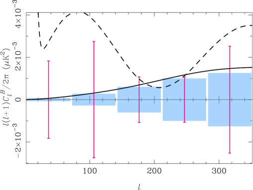
Figure 9: Sample variance errors on the recovered $\hat{C}_{l}^{B}$ using the estimator (53) in the null hypothesis $r=0$. The survey area and weight function are the same as in Fig. 8. The error boxes are the contribution purely from $C_{l}^{B}$ (i.e. the lens-induced $B$ modes) to the one-sigma errors on flat bandpower estimates with a $\varDelta l=70$. These are thus representative of the errors that would be obtained with the pseudo-$C_{l}$ method if it were applied to maps from which the $E$ modes had been removed (see Sect. 6.4, but here we have ignored the loss of information to the ambiguous modes). The error bars are the contribution purely from $C_{l}^{E}$ and arise from $E$-$B$ mixing. The dashed and solid lines are crude ‘rule-of-thumb’ approximations to the errors; see adc:challinor04 for full details.

An important issue for heuristically-weighted quadratic estimators is that the weighting scheme adopted generally makes no attempt to separate $E$ and $B$ modes coherently. While we can remove $E$-$B$ mixing from the power spectra in the mean, in any realisation $\hat{C}_{l}^{B}$ need not vanish even if there are no $B$-modes present. This cross-contribution to the sample variance of pseudo-$C_{l}$ estimators makes them inaccurate for high-sensitivity, small-area $B$-mode surveys. This is illustrated in Fig. 9, where it is shown that the contribution to the sample variance of $\hat{C}_{l}^{B}$ due to leakage of $E$ modes is well in excess of that due to lens-induced $B$ modes. (We have assumed there are no gravitational waves present, so lensing is the only source of $B$ modes.) For the $15^{\circ}$-radius survey considered, with no instrument noise, this excess variance increases the error on the tensor-to-scalar ratio $r$ in the null hypothesis to $\varDelta r=0.15$ ($3\sigma$). One way to remove this problem is first to isolate the $B$ modes with the methods described in Sect. 6.4. Ignoring the loss in this process, we find that the limit on $r$ is then reduced to $3.0\times 10^{-4}$; this arises solely from the sample variance of the lens-induced $B$ modes.

6.6 Non-Gaussianity and lensing reconstruction

The effect of lensing on the CMB will probably be seen first in the angular power spectra (e.g. adc:zaldarriaga98lens ; adc:seljak96 and references therein), or, indirectly, via cross-correlation with large-scale structure adc:hirata04 . As with gravitational-wave searches, the most promising place to look from the standpoint of cosmic variance is the $B$-mode spectrum since, on small scales, lensing may be the dominant signal. Lensing is sensitive to the evolution of the gravitational potential at low redshift and can thus can be used to probe parameters, such as neutrino masses and the properties of dark energy, to which the primary CMB spectra are insensitive adc:hu02synergy . At the sensitivity of the Planck experiment, the effect of lensing on the observed power spectra must be included to avoid bias when estimating parameters such as the baryon density. As thermal noise levels improve, and the sample variance of lens-induced $B$-modes comes to dominate the error budget on $C_{l}^{B}$, corrections due to the non-Gaussianity from lensing will need to be included in the $C_{l}^{B}$ errors and their covariance adc:smith04 .

Looking further ahead, a number of authors have proposed reconstructing the lensing deflection field directly from the CMB by exploiting the non-Gaussianity of the lensing effect (see e.g. adc:seljak99lensrecon ; adc:hu01lensrecon and references therein). This allows one to extract more information from the observed (lensed) CMB fields than is possible with an analysis of their power spectra alone, as well as providing a coherent reconstruction of the projected mass distribution. In essence, the reconstruction methods work by using the locally-anisotropic effect of lensing shear on the statistics of the CMB fluctuations within a region over which the deflections are coherent ($\sim 60^{\circ}$). The fact that we do not know the unlensed CMB fields, but only their statistical properties, introduces a noise in the reconstruction analogous to the effect of the scatter in intrinsic ellipticities of background galaxies in cosmic shear analyses. CMB polarization is particularly useful here adc:benabed01 ; adc:hu02lensrecon ; adc:hirata03 : it has more power on small scales than the temperature anisotropies and so allows reconstruction of the deflection to smaller scales. It was shown in adc:hu02lensrecon that local correlations between $E$ and the lens-induced $B$ modes, estimated with simple quadratic estimators, reconstruct the deflection field with the highest signal-to-noise on all scales once thermal noise permits imaging of the lens-induced $B$ modes on small scales. This requires both high sensitivity ($\sim 1\,\mu\mathrm{K}$ in an arcmin pixel), and also high angular resolution (a few arcmin). The $E$-$B$ estimator is particularly powerful since there is no contribution to its sample variance from chance correlations in the unlensed fields since there are no unlensed small-scale $B$ modes.

Recently, it has been argued that the relatively larger non-Gaussianity of the small-scale (lensed) $B$-modes, compared to the temperature anisotropies and $E$ modes, allows further improvement in the lensing reconstruction if more optimal techniques are employed adc:hirata03 . Indeed, a simple counting argument suggests that, in the absence of thermal noise, the assumption that lensing is the only source of small-scale $B$ modes allows perfect reconstruction of the deflection field (except possibly for a few degenerate configurations). In practice, errors in the theoretical modelling of lensing ultimately limit the reconstruction, but this effect is unimportant until thermal noise levels fall well below the very optimistic level of $0.25\,\mu$K-arcmin.

An important application of lensing reconstruction is to ‘clean out’ the large-scale $B$ modes where any gravitational wave background is expected to contribute. If the lens-induced modes are treated simply as an additional source of Gaussian confusion, the limit on the detectability imposed by lensing (i.e. with no thermal noise or errors in foreground removal) is $r>4\times 10^{-5}$ at $3\sigma$ for a full-sky survey adc:knox02 . This can be improved by more than a factor of 40 with optimal reconstruction methods adc:seljak04lens , corresponding to an energy scale of inflation $V^{1/4}\approx 1\times 10^{15}\,\mathrm{GeV}$.

7 Conclusion

Detections of CMB polarization are still at an early stage, but already we are beginning to see the promise of polarization data for constraining cosmological models being realised. The electric-polarization power spectrum measurements from DASI adc:leitch04 and CBI adc:readhead04 reveal acoustic oscillations with an amplitude and phase perfectly consistent with the best-fit adiabatic models to the temperature anisotropies. This is a non-trivial test on the dynamics of the photons and baryons around the time of recombination. Furthermore, the large-angle measurements of the temperature–polarization cross-correlation from WMAP adc:kogut03 indicate a large optical depth to reionization and hence a complex ionization history. We can expect further rapid progress observationally, with more accurate measurements of the power spectra of $E$-mode polarization, and its correlation with the temperature anisotropies, expected shortly from a number of ground and balloon-borne experiments. These experiments will also greatly increase our knowledge of polarized astrophysical foregrounds at CMB frequencies. Instruments are currently being commissioned that should have the sensitivity to detect the power of $B$-mode polarization induced by weak gravitational lensing adc:bowden04 , and, already, several groups are working on a new generation of polarimeters with the ambition of detecting gravitational-waves and reconstructing the projected mass distribution from CMB polarization observations.

The success of these programmes will depend critically on many complex data analysis steps. We have attempted to summarise here some of the generic parts of a polarization data analysis pipeline, but, inevitably, have had to leave out many topics that are more instrument-specific. Important omissions include calibration of the instrument, cleaning and other low-level reductions of time-stream data, noise estimation, propagation of errors, and the broad topic of statistical accounting for non-ideal instrument effects. Given the exquisite control of systematic effects – both instrumental and astrophysical – that searching for sub-$\mu\mathrm{K}$ signals demands adc:hu03systematic , these omissions will almost certainly prove to be the most critical steps.

References

- (1) C.L. Bennett et al: Astrophysical. J. Suppl. 148, 97 (2003)
- (2) J.R. Bond, C.R. Contaldi, D. Pogoysan: Phil. Trans. R. Soc. Lond. A 361, 2435 (2003)
- (3) A.H. Guth: Phys. Rev. D 23, 347 (1981)
- (4) M.J. Rees: Astrophysical. J. Lett. 153, 1 (1968)
- (5) J.M. Kovac et al: Nature 420, 772 (2002)
- (6) A.C.S. Readhead et al: Science 306, 836 (2004)
- (7) D. Barkats et al: Astrophysical. J. Lett. 619, 127 (2005)
- (8) A. Kogut, D.N. Spergel, C. Barnes: Astrophysical. J. Suppl. 148, 161 (2003)
- (9) M. Zaldarriaga, D.N. Spergel, U. Seljak: Astrophysical. J. 488, 1 (1997)
- (10) M. Zaldarriaga: Phys. Rev. D 55, 1822 (1997)
- (11) U. Seljak, M. Zaldarriaga: Phys. Rev. Lett. 78, 2054 (1997)
- (12) M. Kamionkowski, A. Kosowsky, A. Stebbins: Phys. Rev. Lett. 78, 2058 (1997)
- (13) M. Bucher, K. Moodley, N. Turok: Phys. Rev. Lett. 87, 191301 (2001)
- (14) J.R. Bond et al: Comput. Sci. Eng. 1, 21 (1999)
- (15) J.N. Goldberg et al: J. Math. Phys. 8, 2155 (1967)
- (16) D.A. Varshalovich, A.N. Moskalev, V.K. Khersonskii: Quantum theory of angular momentum, (World Scientific, Singapore 1988) pp 72–117
- (17) A. de Oliveira-Costa et al: Phys. Rev. D 69, 063516 (2004)
- (18) P. Vielva et al: Astrophysical. J. 609, 22 (2004)
- (19) C.J. Copi, D. Huterer, G.D. Starkman: Phys. Rev. D 70, 043515 (2004)
- (20) H.K. Eriksen et al: Astrophysical. J. 605, 14 (2004)
- (21) F.K. Hansen et al: Astrophysical. J. Lett. 607, 67 (2004).
- (22) D.J. Schwarz et al: Phys. Rev. Lett. 93, 221301 (2004)
- (23) D. Coulson, R.G. Crittenden, N.G. Turok: Phys. Rev. Lett. 73, 2390 (1994)
- (24) K. Ng, G. Liu: Int. J. mod. Phys. D 8, 61 (1999)
- (25) G. Chon et al: Mon. Not. R. Astron. Soc. 350, 914 (2004)
- (26) M. Zaldarriaga, U. Seljak: Phys. Rev. D 55, 1830 (1997)
- (27) D. Scott, M. Srednicki, M. White: Astrophysical. J. Lett. 421, 5 (1994)
- (28) M.P. Hobson, J. Magueijo: Mon. Not. R. Astron. Soc. 283, 1133 (1996)
- (29) M. Tegmark: Mon. Not. R. Astron. Soc. textbf280, 299 (1996)
- (30) D.N. Spergel et al: Astrophysical. J. Suppl. 148, 175 (2003)
- (31) W. Hu, M. White: Phys. Rev. D 56, 596 (1997)
- (32) A. Challinor: Phys. Rev. D 62, 043004 (2000)
- (33) W. Hu, M. White: New Astronomy 2, 323 (1997)
- (34) A. Lewis, A. Challinor, A. Lasenby: Astrophysical. J. 538, 473 (2000)
- (35) M. Zaldarriaga, U. Seljak: Phys. Rev. D 58, 023003 (1998)
- (36) E.M. Leitch et al: preprint astro-ph/0409357, (2004)
- (37) B.G. Keating et al: Astrophysical. J. Lett. 560, 1 (2001)
- (38) U. Seljak et al: preprint astro-ph/0407372, (2004)
- (39) H.V. Peiris et al: Astrophysical. J. Suppl. 148, 213 (2003)
- (40) C. Gordon, A. Lewis: Phys. Rev. D 67, 123513 (2003)
- (41) M. Bucher et al: Phys. Rev. Lett. 93, 081301 (2004)
- (42) G.P. Holder et al: Astrophysical. J. 595, 13 (2003)
- (43) W. Hu, G.P. Holder: Phys. Rev. D textbf68, 023001 (2003)
- (44) L. Knox, Y. Song: Phys. Rev. Lett. 89, 011303 (2002)
- (45) M. Kesden, A. Cooray, M. Kamionkowski: Phys. Rev. Lett. 89, 011304 (2002)
- (46) U. Seljak, C.M. Hirata: Phys. Rev. D 69, 043005 (2004)
- (47) P.J. Steinhardt, N. Turok: Science 296, 1436 (2002)
- (48) L.A. Boyle, P.J. Steinhardt, N. Turok: Phys. Rev. D 69, 127302 (2004)
- (49) N. Jones, H. Stoica, S.-H.H. Tye: J. High Energy Phys. 7, 51 (2002)
- (50) U. Seljak, U. Pen, N. Turok: Phys. Rev. Lett. 79, 1615 (1997)
- (51) L. Pogosian et al: Phys. Rev. D 68, 023506 (2003)
- (52) A. Lewis: Phys. Rev. D 70, 043011 (2004)
- (53) A. Kosowsky, A. Loeb: Astrophysical. J. 469, 1 (1996)
- (54) E.S. Scannapieco, P.G. Ferreira: Phys. Rev. D 56, 7493 (1997)
- (55) A. Kosowsky et al: preprint astro-ph/0409767, (2004)
- (56) W. Hu: Phys. Rev. D 65, 023003 (2002)
- (57) J.R. Bond, R. Crittenden: CMB Analysis. In: NATO ASIC Proc. 565: Structure Formation in the Universe, ed by R. Crittenden, N.G. Turok (Kluwer Academic Publishers, Dordrecht 2001) pp 241–280
- (58) A. Challinor et al: Phys. Rev. D 62, 123002 (2000)
- (59) R. Stompor et al: Phys. Rev. D 65, 022003 (2002)
- (60) J. Delabrouille: Astron. Astrophys. Suppl. 127, 555 (1998)
- (61) M. Zaldarriaga: Phys. Rev. D 64, 103001 (2001)
- (62) A.R. Duncan et al: Mon. Not. R. Astron. Soc. 291, 279 (1997)
- (63) W.N. Brouw, T.A.T. Spoelstra: Astron. Astrophys. Suppl. 26, 129 (1976)
- (64) G. Bernardi et al: Astrophysical. J. Lett. 594, 5 (2003)
- (65) G. Giardino et al: Astron. Astrophys. 387, 82 (2002)
- (66) N. Ponthieu et al: preprint astro-ph/0501427, (2005)
- (67) F.R. Bouchet, S. Prunet, S.K. Sethi: Mon. Not. R. Astron. Soc. 302, 663 (1999)
- (68) C. Baccigalupi et al: preprint astro-ph/0209591, (2002)
- (69) J. Delabrouille, J.-F. Cardoso, G. Patanchon: Mon. Not. R. Astron. Soc. 346, 1089 (2003)
- (70) M. Tucci et al: preprint astro-ph/0411567, (2004)
- (71) E.F. Bunn et al: Phys. Rev. D 67, 023501 (2003)
- (72) A. Lewis, A. Challinor, N. Turok: Phys. Rev. D 65, 023505 (2002)
- (73) A. Lewis: Phys. Rev. D 68, 083509 (2003)
- (74) K.M. Smith, W. Hu, M. Kaplinghat: Phys. Rev. D 70, 043002 (2004)
- (75) J.R. Bond, A.H. Jaffe, L. Knox: Phys. Rev. D 57, 2117 (1998)
- (76) B.D. Wandelt, E. Hivon, K.M. Górski: Phys. Rev. D 64, 083003 (2001)
- (77) E. Hivon et al: Astrophysical. J. 567, 2 (2002)
- (78) I. Szapudi, S. Prunet, S. Colombi: Astrophysical. J. Lett. 561, 11 (2001)
- (79) G. Efstathiou: Mon. Not. R. Astron. Soc. 349, 603 (2004)
- (80) M. Tegmark: Phys. Rev. D 55, 5895 (1997)
- (81) M. Tegmark, A. de Oliveira-Costa: Phys. Rev. D 64, 063001 (2001)
- (82) F.K. Hansen, K.M. Górski: Mon. Not. R. Astron. Soc. 343, 559 (2003)
- (83) K.M. Gorski et al: preprint astro-ph/0409513 (2004)
- (84) A. Challinor, G. Chon: preprint astro-ph/0410097 (2004)
- (85) G. Hinshaw et al: Astrophysical. J. Suppl. 148, 135 (2003)
- (86) R.G. Crittenden et al: Astrophysical. J. 568, 20 (2002)
- (87) M.L. Brown, P.G. Castro, A.N. Taylor: preprint astro-ph/0410394, (2004)
- (88) U. Seljak: Astrophysical. J. 463, 1 (1996)
- (89) C.M. Hirata et al: Phys. Rev. D 70, 103501 (2004)
- (90) U. Seljak, M. Zaldarriaga: Phys. Rev. Lett. 82, 2636 (1999)
- (91) W. Hu: Astrophysical. J. Lett. 557, 79 (2001)
- (92) K. Benabed, F. Bernardeau, L. van Waerbeke: Phys. Rev. D 63, 043501 (2001)
- (93) W. Hu, T. Okamoto: Astrophysical. J. 574, 566 (2002)
- (94) C.M. Hirata, U. Seljak: Phys. Rev. D 68, 083002 (2003)
- (95) M. Bowden et al: Mon. Not. R. Astron. Soc. 349, 321 (2004)
- (96) W. Hu, M.M. Hedman, M. Zaldarriaga: Phys. Rev. D 67, 043004 (2003)