A Northern Sky Survey for Steady TeV Gamma-Ray Point Sources Using the Tibet Air Shower Array

M. Amenomori¹¹affiliation: Department of Physics, Hirosaki University, Hirosaki 036-8561, Japan , S. Ayabe²²affiliation: Department of Physics, Saitama University, Saitama 338-8570, Japan , D. Chen³³affiliation: Faculty of Engineering, Yokohama National University, Yokohama 240-8501, Japan , S.W. Cui²⁰²⁰affiliation: Department of Physics, HeBei Normal University, Shijiazhuang 050016, China , Danzengluobu⁵⁵affiliation: Department of Mathematics and Physics, Tibet University, Lhasa 850000, China , L.K. Ding⁴⁴affiliation: Key Laboratory of Particle Astrophysics, Institute of High Energy Physics, Chinese Academy of Sciences, Beijing 100049, China , X.H. Ding⁵⁵affiliation: Department of Mathematics and Physics, Tibet University, Lhasa 850000, China , C.F. Feng⁶⁶affiliation: Department of Physics, Shandong University, Jinan 250100, China , Z.Y. Feng⁷⁷affiliation: Institute of Modern Physics, South West Jiaotong University, Chengdu 610031, China , X.Y. Gao⁸⁸affiliation: Department of Physics, Yunnan University, Kunming 650091, China , Q.X. Geng⁸⁸affiliation: Department of Physics, Yunnan University, Kunming 650091, China , H.W. Guo⁵⁵affiliation: Department of Mathematics and Physics, Tibet University, Lhasa 850000, China , H.H. He⁴⁴affiliation: Key Laboratory of Particle Astrophysics, Institute of High Energy Physics, Chinese Academy of Sciences, Beijing 100049, China , M. He⁶⁶affiliation: Department of Physics, Shandong University, Jinan 250100, China , K. Hibino⁹⁹affiliation: Faculty of Engineering, Kanagawa University, Yokohama 221-8686, Japan , N. Hotta¹⁰¹⁰affiliation: Faculty of Education, Utsunomiya University, Utsunomiya 321-8505, Japan , Haibing Hu⁵⁵affiliation: Department of Mathematics and Physics, Tibet University, Lhasa 850000, China , H.B. Hu⁴⁴affiliation: Key Laboratory of Particle Astrophysics, Institute of High Energy Physics, Chinese Academy of Sciences, Beijing 100049, China , J. Huang¹¹¹¹affiliation: Institute for Cosmic Ray Research, University of Tokyo, Kashiwa 277-8582, Japan , Q. Huang⁷⁷affiliation: Institute of Modern Physics, South West Jiaotong University, Chengdu 610031, China , H.Y. Jia⁷⁷affiliation: Institute of Modern Physics, South West Jiaotong University, Chengdu 610031, China , F. Kajino¹²¹²affiliation: Department of Physics, Konan University, Kobe 658-8501, Japan , K. Kasahara¹³¹³affiliation: Faculty of Systems Engineering, Shibaura Institute of Technology, Saitama 330-8570, Japan , Y. Katayose³³affiliation: Faculty of Engineering, Yokohama National University, Yokohama 240-8501, Japan , C. Kato¹⁴¹⁴affiliation: Department of Physics, Shinshu University, Matsumoto 390-8621, Japan , K. Kawata¹¹¹¹affiliation: Institute for Cosmic Ray Research, University of Tokyo, Kashiwa 277-8582, Japan , Labaciren⁵⁵affiliation: Department of Mathematics and Physics, Tibet University, Lhasa 850000, China , G.M. Le¹⁵¹⁵affiliation: Center of Space Science and Application Research, Chinese Academy of Sciences, Beijing 100080, China , J.Y. Li⁶⁶affiliation: Department of Physics, Shandong University, Jinan 250100, China , H. Lu⁴⁴affiliation: Key Laboratory of Particle Astrophysics, Institute of High Energy Physics, Chinese Academy of Sciences, Beijing 100049, China , S.L. Lu⁴⁴affiliation: Key Laboratory of Particle Astrophysics, Institute of High Energy Physics, Chinese Academy of Sciences, Beijing 100049, China , X.R. Meng⁵⁵affiliation: Department of Mathematics and Physics, Tibet University, Lhasa 850000, China , K. Mizutani²²affiliation: Department of Physics, Saitama University, Saitama 338-8570, Japan , J. Mu⁸⁸affiliation: Department of Physics, Yunnan University, Kunming 650091, China , K. Munakata¹⁴¹⁴affiliation: Department of Physics, Shinshu University, Matsumoto 390-8621, Japan , A. Nagai¹⁶¹⁶affiliation: Advanced Media Network Center, Utsunomiya University, Utsunomiya 321-8585, Japan , H. Nanjo¹¹affiliation: Department of Physics, Hirosaki University, Hirosaki 036-8561, Japan , M. Nishizawa¹⁷¹⁷affiliation: National Institute for Informatics, Tokyo 101-8430, Japan , M. Ohnishi¹¹¹¹affiliation: Institute for Cosmic Ray Research, University of Tokyo, Kashiwa 277-8582, Japan , I. Ohta¹⁰¹⁰affiliation: Faculty of Education, Utsunomiya University, Utsunomiya 321-8505, Japan , H. Onuma²²affiliation: Department of Physics, Saitama University, Saitama 338-8570, Japan , T. Ouchi⁹⁹affiliation: Faculty of Engineering, Kanagawa University, Yokohama 221-8686, Japan , S. Ozawa¹¹¹¹affiliation: Institute for Cosmic Ray Research, University of Tokyo, Kashiwa 277-8582, Japan , J.R. Ren⁴⁴affiliation: Key Laboratory of Particle Astrophysics, Institute of High Energy Physics, Chinese Academy of Sciences, Beijing 100049, China , T. Saito¹⁸¹⁸affiliation: Tokyo Metropolitan College of Aeronautical Engineering, Tokyo 116-0003, Japan , M. Sakata¹²¹²affiliation: Department of Physics, Konan University, Kobe 658-8501, Japan , T. Sasaki⁹⁹affiliation: Faculty of Engineering, Kanagawa University, Yokohama 221-8686, Japan , M. Shibata³³affiliation: Faculty of Engineering, Yokohama National University, Yokohama 240-8501, Japan , A. Shiomi¹¹¹¹affiliation: Institute for Cosmic Ray Research, University of Tokyo, Kashiwa 277-8582, Japan , T. Shirai⁹⁹affiliation: Faculty of Engineering, Kanagawa University, Yokohama 221-8686, Japan , H. Sugimoto¹⁹¹⁹affiliation: Shonan Institute of Technology, Fujisawa 251-8511, Japan , M. Takashima¹²¹²affiliation: Department of Physics, Konan University, Kobe 658-8501, Japan M. Takita¹¹¹¹affiliation: Institute for Cosmic Ray Research, University of Tokyo, Kashiwa 277-8582, Japan , Y.H. Tan⁴⁴affiliation: Key Laboratory of Particle Astrophysics, Institute of High Energy Physics, Chinese Academy of Sciences, Beijing 100049, China , N. Tateyama⁹⁹affiliation: Faculty of Engineering, Kanagawa University, Yokohama 221-8686, Japan , S. Torii⁹⁹affiliation: Faculty of Engineering, Kanagawa University, Yokohama 221-8686, Japan , H. Tsuchiya¹¹¹¹affiliation: Institute for Cosmic Ray Research, University of Tokyo, Kashiwa 277-8582, Japan , S. Udo¹¹¹¹affiliation: Institute for Cosmic Ray Research, University of Tokyo, Kashiwa 277-8582, Japan , T. Utsugi⁹⁹affiliation: Faculty of Engineering, Kanagawa University, Yokohama 221-8686, Japan , H. Wang⁴⁴affiliation: Key Laboratory of Particle Astrophysics, Institute of High Energy Physics, Chinese Academy of Sciences, Beijing 100049, China , X. Wang²²affiliation: Department of Physics, Saitama University, Saitama 338-8570, Japan , Y.G. Wang⁶⁶affiliation: Department of Physics, Shandong University, Jinan 250100, China , H.R. Wu⁴⁴affiliation: Key Laboratory of Particle Astrophysics, Institute of High Energy Physics, Chinese Academy of Sciences, Beijing 100049, China , L. Xue⁶⁶affiliation: Department of Physics, Shandong University, Jinan 250100, China , Y. Yamamoto¹²¹²affiliation: Department of Physics, Konan University, Kobe 658-8501, Japan , C.T. Yan⁴⁴affiliation: Key Laboratory of Particle Astrophysics, Institute of High Energy Physics, Chinese Academy of Sciences, Beijing 100049, China , X.C. Yang⁸⁸affiliation: Department of Physics, Yunnan University, Kunming 650091, China , S.Yasue¹⁴¹⁴affiliation: Department of Physics, Shinshu University, Matsumoto 390-8621, Japan , Z.H. Ye¹⁵¹⁵affiliation: Center of Space Science and Application Research, Chinese Academy of Sciences, Beijing 100080, China , G.C. Yu⁷⁷affiliation: Institute of Modern Physics, South West Jiaotong University, Chengdu 610031, China , A.F. Yuan⁵⁵affiliation: Department of Mathematics and Physics, Tibet University, Lhasa 850000, China , T. Yuda¹¹¹¹affiliation: Institute for Cosmic Ray Research, University of Tokyo, Kashiwa 277-8582, Japan , H.M. Zhang⁴⁴affiliation: Key Laboratory of Particle Astrophysics, Institute of High Energy Physics, Chinese Academy of Sciences, Beijing 100049, China , J.L. Zhang⁴⁴affiliation: Key Laboratory of Particle Astrophysics, Institute of High Energy Physics, Chinese Academy of Sciences, Beijing 100049, China , N.J. Zhang⁶⁶affiliation: Department of Physics, Shandong University, Jinan 250100, China , X.Y. Zhang⁶⁶affiliation: Department of Physics, Shandong University, Jinan 250100, China , Yi Zhang⁴⁴affiliation: Key Laboratory of Particle Astrophysics, Institute of High Energy Physics, Chinese Academy of Sciences, Beijing 100049, China , Y. Zhang⁴⁴affiliation: Key Laboratory of Particle Astrophysics, Institute of High Energy Physics, Chinese Academy of Sciences, Beijing 100049, China , Zhaxisangzhu⁵⁵affiliation: Department of Mathematics and Physics, Tibet University, Lhasa 850000, China , and X.X. Zhou⁷⁷affiliation: Institute of Modern Physics, South West Jiaotong University, Chengdu 610031, China
(The Tibet AS

{\bf\gamma}

Collaboration)

Abstract

Results on steady TeV $\gamma$ -ray point source search using data taken from the Tibet HD (Feb. 1997 – Sep. 1999) and Tibet III (Nov. 1999 – Oct. 2001) arrays are presented. From $0^{\circ}$ to $60^{\circ}$ in declination, significant excesses from the well-known steady source Crab Nebula and the high state of the flare type source Markarian 421 are observed. Because the levels of significance from other positions are not sufficiently high, 90% confidence level upper limits on the flux are set assuming different power law spectra. To allow crosschecking, two independently developed analyses are used in this work.

gamma-rays, all-sky survey, point sources

1 Introduction

In the last 15 years, Imaging Atmospheric Cherenkov Telescopes (IACT) have discovered more than 10 sources in TeV energy range populating from pulsar nebula, supernova remnants, starburst galaxies, AGNs of BL Lac type and even a newly found unidentified source Ong (2003); Horan et al. (2004); Weeks (2003); V ${\rm\ddot{o}}$ lk (2003), and it is remarkable that AGNs make up a large percentage of these sources. To understand the mechanism of the TeV $\gamma$ -ray emissions from diversity of objects, and more fundamentally, to understand the origin and acceleration of cosmic ray (CR), it is important that the number of TeV sources will be largely increased. However, to improve the statistics of TeV sources is not a trivial task for IACT due to its small field of view and low duty cycle, which particularly limit its power in detecting flare type sources and unknown sources. Therefore, a complementary detecting technology is necessary. Although their sensitivity for detecting dim $\gamma$ -ray sources is lower than that of the IACT, Extensive Air Shower (EAS) experiments, such as the Tibet air shower array Amenomori et al. (1999, 2000, 2003) and Milagrito/Milagro (Atkins et al. 1999; Atkins et al. 2003; Atkins et al. 2004) experiments, have resulted in successful observation of $\gamma$ -ray emissions from standard candle Crab nebula and from transient sources such as Mrk 501 and Mrk 421. Their characteristic abilities in high duty cycle and large field of view allow them to simultaneously monitor a larger area in space over continuous time. Most importantly, the EAS technique can potentially provide useful information for IACT observatories for their further dedicated observations. Such follow-up observations have been performed by Whipple experiment Falcone et al. 2003a ; Walker et al. 2003b guided by the hot spots seen from TeV $\gamma$ -ray all-sky survey results published by the Tibet air shower array Amenomori et al. 2001a ; Cui et al. (2003) and Milagro Sinnis et al. (2002) experiments.

The satellite experiment EGRET on board the Compton Gamma Ray Observatory (CGRO) pioneered the all-sky $\gamma$ -ray survey in the energy range of 20 MeV to 30 GeV Hartman et al. (1999). The successful detection of the diffuse $\gamma$ -ray emissions from the galactic plane and a peak near 70 MeV seen in a rather hard $\gamma$ -ray spectrum supported the supernova acceleration model, according to which TeV $\gamma$ -ray emissions were also expected. In addition, EGRET discovered 271 $\gamma$ -ray point sources Hunter et al. (1997), among which about 100 were identified as SNRs, AGNs, etc., while the rest has remained unidentified. The diverse types of $\gamma$ -ray emissions, which included galactic sources and extragalactic sources, greatly improved our knowledge of both CR physics and astrophysics.

The all-sky survey remains one of the major concerns for ground-based observatories (Weeks et al. 1989; Alexandreas et al. 1991; Mckay et al. 1993; Wang et al. 2001; Aharonian et al. 2002a; Aharonian et al. 2002b; Atkins et al. 2004; Antoni et al. 2004). For example, AIROBICC made a northern sky survey Aharonian et al. 2002a on $\gamma$ -ray emissions for energy above 15 TeV; because there was no compelling evidence for a signal source, an absolute flux upper limit between 4.2 and 8.8 Crab was obtained for a declination (Decl.) of $0^{\circ}$ and $60^{\circ}$ . With the IACT technique, within the TeV energy range, the HEGRA telescope was used to performe a survey Aharonian et al. 2002b in one quarter of the galactic plane in the longitude range from $-2^{\circ}$ to $85^{\circ}$ . As a result of negative evidence, upper flux limits on each individual known point source located in this region were obtained between 0.15 Crab and several Crab. Most recently, Milagro updated its results Atkins et al. (2004) in the northern sky survey in TeV energy range, and pushed the average flux upper limit down to a level between 275 and 600 mcrab ( $4.8\times 10^{-12}$ to $10.5\times 10^{-12}{\rm cm}^{-2}{\rm s}^{-1}$ ) above 1 TeV for source Decl. between $5^{\circ}$ and $70^{\circ}$ . As an independent experiment, the Tibet air shower array has similar sensitivity, and covers almost the same energy ranges and field of view as those experiments do. The results from the Tibet air shower array should therefore provide important information for crosschecking and confirmation.

2 Tibet Air Shower Observatory

The Tibet air shower array has been conducted at Yangbajing ( $90.522^{\circ}$ E, $30.102^{\circ}$ N; 4,300 m a.s.l) in Tibet, China since 1990. The Tibet I array Amenomori et al. (1992), which consisted of 49 scintillation counters forming a $7\times 7$ matrix of 15 m span, was gradually expanded to the Tibet II array occupying an area of 36,900 m² by increasing the number of counters from 1994 to 1996. Both Tibet I and II have the same mode energy (the most probable gamma ray energy observed from the standard candle Crab) of 10 TeV. In order to observe TeV CRs, in 1996, part of the Tibet II array covering an area of 5,175 m² was further upgraded to a high density (HD) array Amenomori et al. 2001b with 7.5 m span. Soon after decreasing the mode energy to 3 TeV, the HD array observed multi-TeV $\gamma$ -ray signals from the Crab Nebula Amenomori et al. (1999) and Mrk 501 Amenomori et al. (2000). To increase the event rate, in 1999, the HD array was enlarged to cover the center part of the Tibet II array as the Tibet III array Amenomori et al. 2001c . The area of Tibet III has reached to 22,050 m² (Figure 1).

As can be shown in Figure 1, the Tibet HD and Tibet III have identical structure except the array size and shape. Each counter has a plastic scintillation plate (BICRON BC-408A) of 0.5 m² in area and 3 cm in thickness, and is equipped with a fast-timing (FT) photomultiplier tube (PMT; Hamamatsu H1161). A 0.5 cm thick lead plate is put on the top of each counter in order to increase the array sensitivity by converting $\gamma$ -rays into electron-positron pairs in the shower Bloomer et al. (1988); Amenomori et al. (1990). The angular resolution of the HD and the Tibet III are about $0.9^{\circ}$ in the energy region above 3 TeV, as estimated from full Monte Carlo (MC) simulation Amenomori et al. (1990); Kasahara (2003) and verified by the moon shadow measurement from observational data Amenomori et al. (1993); Amenomori et al. 2001c ; Amenomori et al. (2003). The trigger rate is about 105 Hz for the HD and 680 Hz for the Tibet III. In this work, the sample includes data obtained by running the HD array for 555.9 live days from Feb. 1997 to Sept. 1999 and the Tibet III array for 456.8 days from Nov. 1999 to Oct. 2001.

The event selection was done by imposing the following four criteria on the reconstructed data: i) each shower event should fire four or more Fast-Time (FT) detectors recording 1.25 or more particles; ii) the estimated shower center location should be inside the array; iii) the sum of the number of particles per m² detected in each detector $\sum\rho_{\rm{FT}}$ should be larger than $15$ ; iv) the zenith angle of the incident direction should be less than $40^{\circ}$ . After applying these cuts and a data quality cut, about 40% of the shower events were selected, results in a total number of events to be about $7.0\times 10^{9}$ .

3 Analysis

Because the Tibet air shower array can not distinguish a $\gamma$ -ray induced shower event from the overwhelming CR background shower events, when tracing and counting the number of events in an “on-source window” centered at a candidate point source direction with a size at the level of angular resolution, the number of background events must be estimated from the observational data recorded in the side band, which is usually referred to as “off-source window”.

Sitting on an almost horizontal plane, the Tibet HD and III have almost azimuth-independent efficiency in receiving the shower events for any given zenith angle. The equi-zenith angle method was therefore developed. In brief, simultaneously collected shower events in the same zenith angle belt can be used to construct the “off-source windows” and to estimate the background for a candidate point source located in the same zenith angle. This method can eliminate various detecting effects caused by instrumental and environmental variations, such as changes in pressure and temperature which are hard to be controlled and intend to introduce systematic error in measurement. In reality, the actual azimuth angle distribution deviates from a uniform one mainly due to the fact that the Tibet HD and III arrays are situated on a slope of about $1.3^{\circ}$ from the southeast to the northwest. Furthermore, a geomagnetic effect in the northern hemisphere causes unequal efficiency between north and south Ivanov et al. (1999). Together with other possible unknown effects, all the steady effects lead to an approximately $2.5\%$ higher event rate from the southerly direction than from the northerly direction. This non-uniformity must be properly accounted for in the following analyses.

For the purpose of crosschecking, two independently developed analyses based on the equi-zenith angle method are used in this work. One is dedicated to a point source search, while the other in addition is sensitive to large-scale anisotropy of the intensity of the CR. A MC study was used to carefully compare the two methods, and the search sensitivities were found to be very comparable. However, the number of the background events estimated by the two methods is different due to the different ways used in choosing the off-source windows (see subsections below in detail). As a result, significance values calculated from the two methods differ by about 0.5 $\sigma$ statistically.

3.1 Method I (short distance equi-zenith angle method)

As a good approximation, the large-scale anisotropy of the CR intensity can be neglected if the “off-source windows” are chosen to be close enough in distance to the “on-source window”, since the CR intensity only changes slowly in the sky. In this analysis, to make sure not to miss any possible unknown source, the surveyed sky has been over-sampled by the following way: the sky is divided into $0.1^{\circ}\times 0.1^{\circ}$ cells, from $0^{\circ}$ to $360^{\circ}$ in Right Ascension (R.A.) and from $0^{\circ}$ to $60^{\circ}$ in Decl. Pointing to the center of those cells, cones with a half opening angle of $0.9^{\circ}$ (for ${\rm E}>3$ TeV) or $0.4^{\circ}$ (for ${\rm E}>10$ TeV) are tested as on-source windows. These cone sizes are chosen to maximize the source search sensitivity Chen et al. (2004). 10 off-source windows of the same shape are symmetrically aligned on both sides of the on-source window, at a zenith angle-dependent step size in order to maintain an angular distance of $2^{\circ}$ between the neighboring off-source windows. In order to avoid signal events related to an on-source window being wrongly counted as a background event, the two off-source windows closest in distance to the on-source window are required to be placed at twice of the step-size from the center of the on-source window. Denoting the number of events in on-source window as $N_{\rm{ON}}$ , and the number of events in the $i$ th off-source window as $N_{\rm{OFF}\it i}$ , without considering the effect from non-uniform azimuth angle distribution, the number of background events can be estimated as

N_{\rm{BG}}=\frac{\sum_{i=1}^{10}N_{\rm{OFF}\it i}}{10}

(1)

When the zenith angle is less than $4.2^{\circ}$ , the 10 off-source windows defined above become to be overlapped. Therefore, data obtained with a zenith angle less than $4.2^{\circ}$ are not used. Since the azimuth angle distribution is not completely flat as discussed earlier, the averaged number of events from off-source windows, $N_{\rm{BG}}$ , as calculated in equation (1) is not an exact description of the background number in the on-source window. Therefore $N_{\rm{BG}}$ needs to be corrected. Giving the fact that azimuth angle distribution remains stable over a period of time that is much longer than the time scale of a day, the effect of the tiny violation of the exact equi-zenith angle condition can thus be determined from the observational data which were taken only a few hours apart from the exposure of the on (off)-source window(s). As a matter of fact, the previous measurement is repeated 35 times (the relevant “on” and “off” source windows are hereafter called “dummy on” and “dummy off” source windows). Together with the on-source window, 35 dummy on-source windows on the orbit which has the same Decl. as the on-source window are defined at regular intervals along R.A. direction, i.e., the dummy on-source windows are located at $\alpha_{\rm{ON}}+10^{\circ}\times j$ , where $\alpha_{\rm{ON}}$ is the R.A. location of the on-source window, and $j$ an index of the repeated measurements which runs from 1 to 35. $N^{{}^{\prime}}_{\rm{ON}\it j}$ and $N^{{}^{\prime}}_{\rm{BG}\it j}$ represent the number of events in the dummy on-source window and its estimated background from the $j$ th measurement, respectively. The correction factor, $\eta$ , due to non-uniform azimuth angle distribution is given by

{\eta}=\frac{\sum_{j=1}^{35}{N^{{}^{\prime}}_{\rm{ON\it j}}}/{35}}{\sum_{j=1}^{35}{N^{{}^{\prime}}_{\rm{BG\it j}}}/{35}}

(2)

As for the Tibet observation, $\eta$ deviates from 1 at an order of $10^{-3}$ depending on the Decl. of the on-source window.

Finally, the corrected estimation of the number of background events is obtained as

{N^{\ast}}_{\rm BG}={\eta}N_{\rm{BG}}

(3)

It is clear that such a correction is free from the systematic uncertainty due to the slow variation of instrumental and environmental effects. Denoting the number of excess events in an on-source window as $N_{\rm S}$ , its uncertainty, $\Delta N_{\rm S}$ , is given by ${\Delta N{\rm s}}^{2}={\Delta N_{\rm{ON}}}^{2}+{\Delta N^{*}_{\rm{BG}}}^{2}$ , where ${\Delta N_{\rm{ON}}}^{2}$ is well approximated by $N_{\rm{BG}}^{*}$ , and $\Delta N_{\rm{BG}}^{*}$ is propagated from the statistic error of $\eta$ and $N_{\rm BG}$ , according to Equation (3), $\Delta{N_{\rm{BG}}^{*}}^{2}={N_{\rm{BG}}^{*}}^{2}(\frac{{\Delta\eta}^{2}}{\eta^{2}}+\frac{{\Delta N_{\rm{BG}}}^{2}}{N_{\rm{BG}}^{2}})$ . Considering the number of off-source window and dummy on(off)-source window, it is not difficult to calculate $\Delta N_{\rm{BG}}^{*}$ as ${N_{\rm{BG}}^{*}}^{2}[(\frac{1}{35}+\frac{1}{350})(\frac{1}{N_{\rm{ON}}})+(\frac{1}{10})(\frac{1}{N_{\rm{ON}}})]=0.1314{N_{\rm{BG}}^{*}}$ . Then we obtain $\Delta N_{\rm S}=1.0637\sqrt{N_{\rm{BG}}^{*}}$ . Because both $N_{\rm{ON}}$ and $N^{*}_{\rm{BG}}$ are statistically large numbers, the significance value can be simply calculated as

S=\frac{N_{\rm ON}-N^{\ast}_{\rm BG}}{1.0637\sqrt{N^{\ast}_{\rm BG}}}

(4)

3.2 Method II (all distance equi-zenith angle method)

Unlike the method described in the previous sub section, this method attempts to exploit the statistics as much as possible from two approaches.

First, shapes of non-uniformly distributed azimuth angle distribution from whole data set are used to do the azimuth correction. To be more precise, after event selection, for each $1^{\circ}$ zenith angle interval between $0^{\circ}$ to $40^{\circ}$ , azimuth angle distributions are filled and normalized, so that the averaged function value is one. Inversing the function and using it as an event weight would keep the total number of events unchanged but make the azimuth angle distribution flat.

Second, all events in the equi-zenith angle belt except those inside the on-source window are taken as off-source events. In this case the large-scale anisotropy effect can no longer be ignored, which leads to the attempt to fit simultaneously the relative CR intensity over the sky within the detector’s field of view.

The idea of this method is that at any moment, for all directions, if we scale down (or up) the number of observed events by dividing them with their relative CR intensity, then statistically, those scaled observed number of events in a zenith angle belt should be equal anywhere. A $\chi^{2}$ function can be built accordingly and the relative intensity of CRs in each direction can be solved by minimizing the $\chi^{2}$ function.

As in the previous method, the celestial space from 0^∘ to 360^∘ in R.A. and from 0^∘ to 60^∘ in Decl. are binned into cells with a bin size of 0.1^∘ in both the R.A. and Decl. directions. In the observer’s coordinates, the zenith angle $\theta$ is divided from 0^∘ to 40^∘ by a step size of 0.08^∘, and the azimuth angle $\phi$ is binned by a zenith angle dependent bin width (0.08^∘/ sin( $\theta$ )). For every local sidereal time (LST) interval bin (24s) $m$ , a cell in ( $\theta$ , $\phi$ ) space $(n,l)$ is mapped to a celestial cell $(\alpha_{i},\,\delta_{j})$ , i.e. R.A. bin $i$ and Decl. bin $j$ , through two discrete coordinate transformation functions $\imath(m,n,l)$ and $\jmath(m,n,l)$ . Therefore, at a certain LST bin $m$ , the number of events accumulated in zenith angle bin $n$ and azimuth angle bin $l$ is directly related to the CR intensity $I(i,j)$ in cell $(i,j)$ of celestial space.

Denoting the number of observed events after azimuth angle correction as $N_{\rm{OBS}}(m,n,l)$ , and the relative intensity of CR as $I$ (i,j), the equi-zenith angle condition leads to the following $\chi^{2}$ function:

\chi^{2}\,=\,\sum_{m,\,n,\,l}\,\frac{\;\Big{[}\,N_{\rm{OBS}}(m,\,n,\,l)\;\Big{/}\;I(i,\>j)\,-\,{\sum_{\,l^{\prime}\neq\,l}\Big{(}N_{\rm{OBS}}(m,\,n,\,l^{\prime})\;/\;I(i^{\prime},\>j^{\prime})}\Big{)}\,\Big{/}\,{\sum_{\,l^{\prime}\neq\,l}1}\;\Big{]}^{2}}{\;N_{\rm{OBS}}(m,\,n,\,l)\;\Big{/}\;{I^{2}(i,\>j)}\,+\,{\sum_{\,l^{\prime}\neq\,l}\Big{(}N_{\rm{OBS}}(m,\,n,\,l^{\prime})\;/\;I^{2}(i^{\prime},\>j^{\prime})}\Big{)}\,\Big{/}\,({\sum_{\,l^{\prime}\neq\,l}1})^{2}}\,

(5)

Here, $(i,j)$ is mapped from $(m,n,l)$ by the above-mentioned transformation functions.

From equation (5), $I(i,\>j)$ and its error $\Delta I(i,j)$ can be solved numerically by the iteration method. As the dimensionless variable $I(i,j)$ is only a relative quantity, and because the detecting efficiency along the Decl. direction can not be absolutely calibrated, we apply the constraint that averaged $I(i,j)$ in each Decl. slices is equal to one.

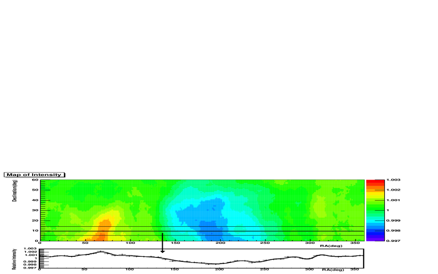
On the other hand, $N(i,j)$ , the number of observed events in the celestial cell $(i,j)$ is simply a summation of the relevant number of events counted in local coordinates $N_{\rm{OBS}}(m,n,l)$ , i.e., $N(i,j)=\sum\limits_{\imath(m,n,l)=i\atop\jmath(m,n,l)=j}N_{\rm{OBS}}(m,n,l)$ .

As the relative intensity of the CR contains the contribution from large-scale anisotropy of the CR, to remove this effect and to isolate the contribution from point sources, the measured CR intensity in a $10^{\circ}$ belt along Decl. is projected to the R.A. direction, in $8^{\circ}$ bin size. The center of the belts moves from $0^{\circ}$ to $60^{\circ}$ , in $1^{\circ}$ step size. By smoothing those curves and subtracting them from the corresponding belt of $1^{\circ}$ width, we obtain a CR intensity, $I_{\rm{CORR}}(i,j)$ , that is corrected for the anisotropy effect.

With this corrected CR intensity, the number of excess events and their uncertainties in cell $(i,j)$ can be calculated as

N_{\rm{S}}(i,j)=\Big{(}I_{\rm{CORR}}(i,j)-1\Big{)}\cdot N(i,j)\,/\,I_{\rm{CORR}}(i,j)

(6)

\triangle N_{\rm{S}}(i,j)=\Delta I_{\rm{CORR}}(i,j)\cdot N(i,j)\,/\,I_{\rm{CORR}}(i,j)

(7)

Taking into account the array’s angular resolution, events are summed up from a cone with an axis pointing to the source direction, and the half opening angle is set as $0.9^{\circ}$ (for ${\rm{E}}>3$ TeV) or $0.4^{\circ}$ (for ${\rm{E}}>10$ TeV). All celestial cells with their centers located inside the cone contribute to the number of events as well as its uncertainty. Finally, the significance for an on-source window centered at cell $(i,j)$ can be calculated as

{\it S}(i,j)\,=\,\frac{\sum\limits_{(i^{\prime},j^{\prime})\in{\rm{CONE}}}\Big{(}(I_{\rm{CORR}}(i^{\prime},j^{\prime})-1)\cdot N(i^{\prime},j^{\prime})\,/\,I_{\rm{CORR}}(i^{\prime},j^{\prime})\Big{)}}{\sqrt{\sum\limits_{(i^{\prime},j^{\prime})\in{\rm{CONE}}}\Big{(}\Delta I_{\rm{CORR}}(i^{\prime},j^{\prime})\cdot N(i^{\prime},j^{\prime})\,/\,I_{\rm{CORR}}(i^{\prime},j^{\prime})\Big{)}^{2}}}\,

(8)

4 Results

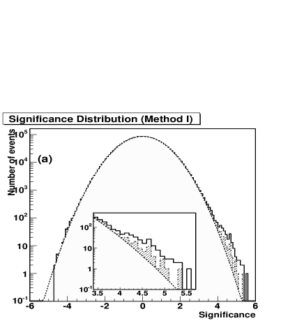
The significance distributions from all directions are shown in Figure 2a and Figure 2b for the two analysis methods, respectively. In the case of method II, the large-scale anisotropy must be measured and subtracted, the systematic uncertainty to the significance value due to this subtraction procedure is estimated to be 0.2 $\sigma$ by changing the bin size and the smoothing parameters. Figure 3 shows the intensity map containing the contribution from the large-scale anisotropy with a demonstration of its subtraction.

The excellent agreement on the negative side with a normal distribution (Figure 2a, Figure 2b) indicates that the systematic effects are well under control for both analyses. As for the positive side, a wider shoulder exists with significance values greater than 4.0 $\sigma$ . The dominant contributions are due to the stable $\gamma$ -ray source Crab and transient source Mrk 421 which was in an active state from Feb. 2000 through Oct. 2001 Amenomori et al. (2003). After removing their contributions, in such a manner that those cells that are less than 2^∘ distance from the two sources are excluded, the dot-dashed histograms in Figure 2a and Figure 2b which show the significance distribution from the rest of the cells agree much better with a normal distribution. For reference, the Table 1 lists the directions of local maximal significance points with significance values greater than 4.5 $\sigma$ from either of the two methods, and those prominent directions contribute to the remaining small shoulder in Figure 2a and Figure 2b.

Each significance value listed in Table 1 is calculated by equation (4) and (8) which is supposed to be used for a predefined on-source window. However, none of our prominent directions comes from a predefined one, as described in section 3.1, a large number of overlapping on-source windows have been tried. In comparison with finding a high significance value from one predefined direction (e.g., Crab or Mrk421), such a procedure makes the probability being larger by a factor of about the number of trials, and therefore making the excess of on-source event number less significant. It should be mentioned that it is very difficult to count the number of trials exactly. To have order of magnitude estimation on the lower boundary of the number of trials, we can divide the solid angle of surveyed sky by the solid angle of one on source window, and get a number of about 7000 which still under estimates the number of trials. As an example, for the first prominent point in Table.1, the significance value is 5.3 $\sigma$ from method I(4.8 $\sigma$ from method II), enlarge the probability by 7000 to account the number of trials effect end up with only 3.3(2.5) $\sigma$ in significance. To distinguish this significance from the previously calculated one, we call the former calculated one the pre-trials significance ( $S_{pre-trials}$ ). This number of trials effect can also be understood from another point of view as the following: not including the Crab and Mrk421, both methods observe four directions which have $S_{pre-trials}$ greater than 4.5 $\sigma$ . From pure background MC simulation, the probability to observe four or more such directions is equivalent to a fluctuation of only 1.4 $\sigma$ . In conclusion, after taking into account the number of trials effect, the existence of the high significance point in Table 1 is well consistent with the background fluctuation.

As can be seen in Table 1, two established sources Crab and Mrk 421 are detected in an angular distance not larger than $0.5^{\circ}$ from their nominal positions, in agree with the $0.4^{\circ}$ positional uncertainty estimated for the both methods. One of our previously reported Cui et al. (2003) hot point with pre-trials significance value of 4.0 $\sigma$ located at ( $304.15^{\circ},36.45^{\circ}$ ) is not listed in Table 1, because its pre-trials significance value is not improved after we further include more data samples into this analysis which increase the number of events by 60%: $4.1$ $\sigma$ from Method I and $4.0$ $\sigma$ from Method II. The interesting thing about this point is that it is close to the Cygnus arm and was found to be close to one of Milargo hot points Walker et al. (2004), though the large angular distance of $1.5^{\circ}$ indicates that the coincidence is not in favour of a point source hypothesis. Conclusive results will rely on further more observation. As a cross-check, Milagro hot point at ( $79.9^{\circ},26.8^{\circ}$ ) Atkins et al. (2004) is investigated in this work: the maximum pre-trials significant point is found at ( $79.3^{\circ},25.9^{\circ}$ ) with $1.3$ $\sigma$ from Method I, and ( $79.9^{\circ},26.3^{\circ}$ ) with $1.7$ $\sigma$ from Method II. In another word, no strong confirmation was obtained. On the other hand, except the agreement measurement with comparable sensitivity on Crab and Mrk 421 from both observatories, no significant prominent direction from this work matches with Milagro hot points Atkins et al. (2004) within the allowed source positional uncertainties. When not considering the Crab and Mrk 421, we think the marginal coincidence and refutation of other hot points between Tibet Air Shower and MILAGRO could be attributed to the limited statistics and sensitivity of the two experiments. Whether these hot points are just due to statistical fluctuation or due to new TeV gamma sources will become clearer with the future improved statistic of observational data.

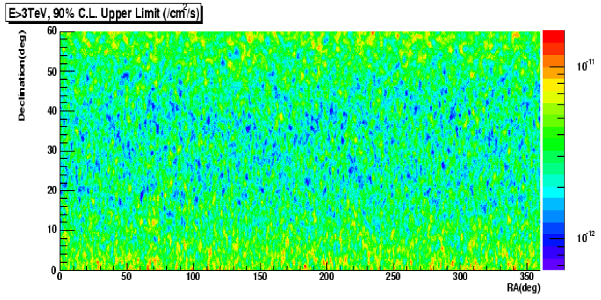
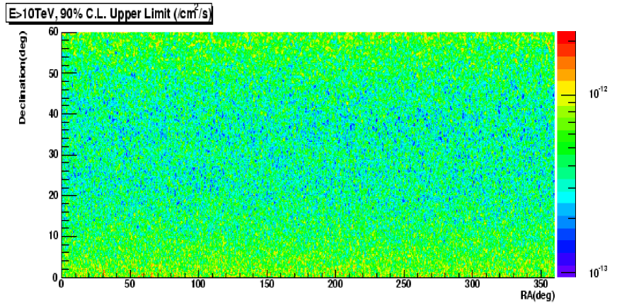
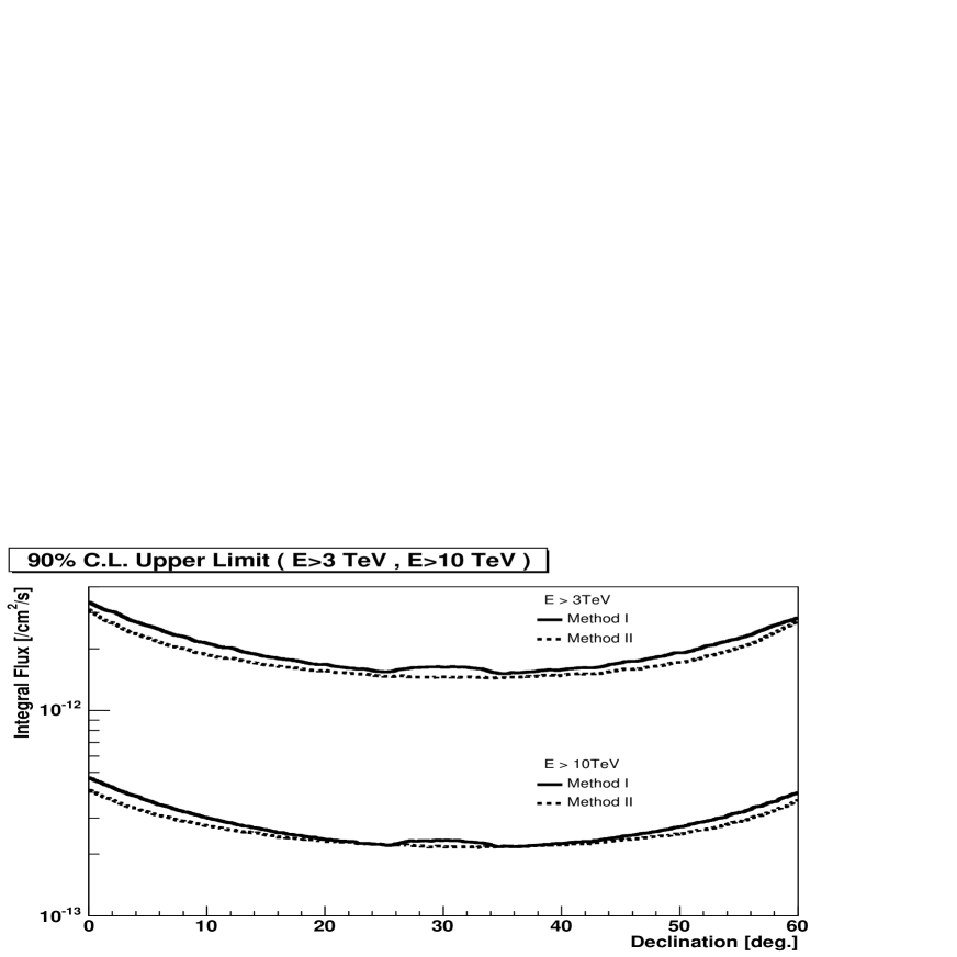
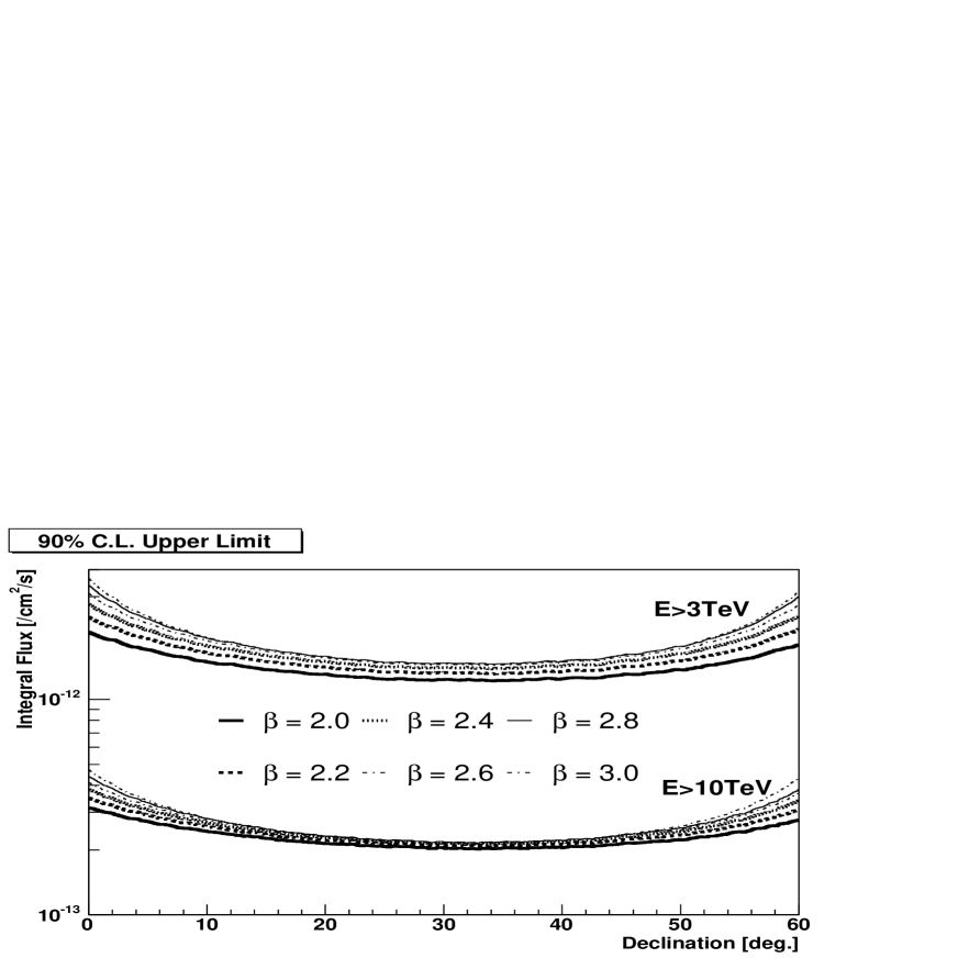
As described previously, the significances from all other directions other than Crab and Mrk 421 are not high enough to definitely claim any existence of new TeV $\gamma$ -ray point source, we set a 90 $\%$ confidence level (CL) upper flux limit for all directions in the sky, except at the positions of Crab and Mrk 421. The upper limit on the number of events at the 90% CL is calculated firstly according to the number of excess events and its uncertainty for each cell following the statistic method given by Helene Helene (1983). Then the effective detection area of Tibet Air Shower array is evaluated by full MC simulation assuming a Crab-like $\gamma$ -ray spectrum ${\rm{E}}^{-\beta}$ with $\beta=2.6$ for a set of Decl. values (0.0^∘, 10.0^∘, 20.0^∘, 30.0^∘, 40.0^∘, 50.0^∘, 60.0^∘) and interpolated to other Decl. values between $0^{\circ}$ and $60^{\circ}$ . Taking into account the live time from observational data taking, we derive the 90% CL flux upper limit. Figure 4 shows the maps of flux upper limits at 90% CL for energy ${\rm{E}}>3$ TeV and for ${\rm{E}}>10$ TeV (from Method I). Figure 5 shows the average flux upper limit along the right ascension direction as a function of Decl., which varies between $1.5-3.2\times 10^{-12}{\rm cm}^{-2}{\rm s}^{-1}$ for ${\rm{E}}>3$ TeV and $0.2-0.4\times 10^{-12}{\rm cm}^{-2}{\rm s}^{-1}$ for ${\rm{E}}>10$ TeV. Current integrated limits for energy above 10 TeV are the world-best ones which improve the results obtained from AIROBICC Aharonian et al. 2002a for energy above 15 TeV. For energy above 3 TeV, limits from this work are comparable with those obtained by Milagro Atkins et al. (2004) for energy above 1 TeV. The same procedure is applied to the cases of other power law indices for energy above 3 TeV and above 10 TeV . The corresponding average flux limit for the other indices can be found in Figure 6 (from method II). Depending on the Decl. and power law index of the candidate source, the integral flux limits lie within $1.5-3.8\times 10^{-12}{\rm cm}^{-2}{\rm s}^{-1}$ ( ${\rm{E}}>3$ TeV) and $0.2-0.48\times 10^{-12}{\rm cm}^{-2}{\rm s}^{-1}$ ( ${\rm{E}}>10$ TeV).

5 Conclusion

A northern sky survey for the TeV $\gamma$ -ray point sources in a Decl. band between $0^{\circ}$ to $60^{\circ}$ was performed using data of the Tibet HD and the Tibet III air shower array obtained from 1997 to 2001 with two independently developed analysis methods. The established Crab and Mrk 421 were observed. This indicates that the Tibet air shower array is a sensitive apparatus for TeV $\gamma$ -ray astronomy and has a potential to find flare type $\gamma$ -ray sources, such as BL-Lac type AGNs. In addition, the 6 other prominent directions were selected. However, more data will be needed before we can confirm or rule out these candidates.

With the exception of Crab and Mrk 421, 90% CL flux upper limits are obtained from the rest of the positions under the hypothesis that a candidate point source are in power law spectra, with indices varying from $2.0$ to $3.0$ . The integral flux limits lie within $1.5-3.8\times 10^{-12}{\rm cm}^{-2}{\rm s}^{-1}$ ( ${\rm{E}}>3$ TeV) and $0.2-0.48\times 10^{-12}{\rm cm}^{-2}{\rm s}^{-1}$ ( ${\rm{E}}>10$ TeV) depending on the Decl. and power law index of the candidate source.

This work is supported in part by Grants-in-Aid for Scientific Research on Priority Areas (712) (MEXT) and by Scientific Research (JSPS) in Japan, and by a grant for International Science Research from the Committee of the Natural Science Foundation and the Chinese Academy of Sciences in China.

References

Alexandreas et al. (1991) Alexandreas, D.E., et al., 1991, ApJ, 383, L53-L56
Amenomori et al. (1990) Amenomori, M., et al. 1990, Nucl. Instrum. Methods Phys. Res., A288, 619
Amenomori et al. (1992) ———. 1992, Phys. Rev. Lett., 69, 2468
Amenomori et al. (1993) ———. 1993, Phy. Rev. D 47, 2675-2681
Amenomori et al. (1999) ———. 1999, ApJ, 525, L93
Amenomori et al. (2000) ———. 2000, ApJ, 532, 302
(7) ———. 2001a, Proc. 27th Int. Cosmic Ray Conf. (Hamburg), 6, 2544
(8) ———. 2001b, AIP, CP558, High Energy Gamma-Ray Astronomy, P557
(9) ———. 2001c, Proc. 27th Int. Cosmic Ray Conf. (Hamburg), 2, 573
Amenomori et al. (2003) ———. 2003, ApJ, 598, 242
(11) Aharonian, F., et al., 2002a, A&A, 390, 39
(12) ———. 2002b, A&A, 395, 803
Antoni et al. (2004) Antoni, T., et al., 2004, ApJ, 608, 865
Atkins et al. (1999) Atkins, R., et al., 1999, ApJ, 525, L25-L28
Atkins et al. (2003) ———. 2003, ApJ, 595, 803-811
Atkins et al. (2004) ———. 2004, ApJ, 608, 680-685
Bloomer et al. (1988) Bloomer, S. D., Linsley, J.,& Watson, A. A. 1988, J. Phys. G, 14, 645
Chen et al. (2004) Chen, X., et al., HEP & NP, 2004, 28(10):1094-1098 (in Chinese)
Cui et al. (2003) Cui, S. W., et al., 2003, Proc. 28th Int. Cosmic Ray Conf. (Tsukuba), 4, 2315.
(20) Falcone, A., et al., 2003a, Proc. 28th Int. Cosmic Ray Conf. (Tsukuba), 5, 2579
Hartman et al. (1999) Hartman, R.C., et al., 1999, ApJS, 123, 79
Helene (1983) Helene, O., 1983, Nucl. Instrum. Methods Phys. Res., 212, 319
Horan et al. (2004) Horan, D., Weeks, T.C., 2004, New Astro. Rev. 48, 527-535
Hunter et al. (1997) Hunter, S.D., et al., 1997, ApJ, 481, 205
Ivanov et al. (1999) Ivanov, A.A., et al., 1999, JETP Lett., 69, 288
Kasahara (2003) Kasahara, K., http://cosmos.n.kanagawa-u.ac.jp/EPICSHome/
Mckay et al. (1993) Mckay, T.A., et al., 1993, ApJ, 417:742-747
Sinnis et al. (2002) Sinnis, C. 2002, proceedings of American physical society and High energy Astrophysics of the AAS Mtg
Ong (2003) Ong, Rene A., 2003, The Universe Viewed in Gamma-Rays, 587 (Universal Academy Press, Tokyo).
V ${\rm\ddot{o}}$ lk (2003) V ${\rm\ddot{o}}$ lk, H.J., 2003, Frontiers of Cosmic Ray Science, 29 ( Universal Academy Press, Tokyo )
(31) Walker, G., et al., 2003b, Proc. 28th Int. Cosmic Ray Conf. (Tsukuba), 5, 2563
Walker et al. (2004) Walker, G., Atkins, R., Kieda, D., 2004, ApJ, 614, L93-L96
Wang et al. (2001) Wang, K. et al., 2001, ApJ, 558, 477
Weeks et al. (1989) Weeks, T.C., et al., 1989, ApJ, 342, 379
Weeks (2003) Weeks, T.C., 2003, Frontiers of Cosmic Ray Science, 3 ( Universal Academy Press, Tokyo )

Table 1: Prominent directions with at least one pre-trials significance value greater than

4.5

\sigma

from either of two methods. Each pre-trials significance values are calculated by the equation (4) or (8).

No.	Method	R.A.(^∘)	Decl.(^∘)	$N_{ON}$	$N_{OFF}$	$N_{S}$	$\Delta N_{s}$	$S_{pre-trials}$
	I	69.95^⋆^⋆ The last digital number in column of R.A. and Decl. are due to the way we divide the bin in the analyses.	12.05	828557.0	823428.5	5128.5	965.2	5.3
1	II	70.25	11.95	825589.0	821232.4	4356.6	906.2	4.8
	I	70.45	18.15	997441.0	992485.7	4955.3	1059.7	4.7
2	II	70.45	18.05	994477.0	990343.3	4133.7	995.2	4.2
	I	83.55	22.25	1087857.0	1082101.0	5756.0	1106.5	5.2
3	II	83.35	21.85	1079728.0	1074562.6	5165.4	1036.6	5.0
	I	88.85	30.25	1013683.0	1008916.9	4766.1	1068.4	4.5
4	II	88.85	30.25	1185535.0	1179647.4	5887.6	1086.1	5.4
	I	165.65	38.45	1170565.0	1164237.2	6327.8	1147.7	5.5
5	II	165.55	38.45	1170632.0	1164908.8	5723.2	1079.3	5.3
	I	221.65	32.85	1062942.0	1057488.1	5453.9	1093.9	5.0
6	II	221.75	32.75	1191295.0	1186765.1	4529.9	1089.4	4.2
	I	286.65	5.45	608892.0	604934.2	3957.8	827.3	4.8
7	II	286.65	5.55	612041.0	608322.9	3718.1	780.0	4.8
	I	309.85	39.65	1146305.0	1141238.9	5066.1	1136.3	4.5
8	II	309.95	39.65	1146636.0	1141544.7	5091.3	1068.4	4.8

Refer to caption — Figure 1: Schematical view of the Tibet III array operating at Yangbajing. Open squares: FT-detectors; filled squares: FT-detectors with a wide dynamic range PMT; filled circles: density detectors with a wide dynamic range PMT. We select air shower events whose cores are located within the detector matrix enclosed with the dashed line.