Cosmological model with energy transfer

Abstract

The observations of SNIa suggest that we live in the acceleration epoch when the densities of the cosmological constant term and matter are almost equal. This leads to the cosmic coincidence conundrum. As the explanation for this problem we propose the FRW model with dark matter and dark energy which interact each other exchanging energy. We show that the cubic correction to the Hubble law, measured by distant supernovae type Ia, probes this interaction. We demonstrate that influences between nonrelativistic matter and vacuum sectors are controlled by third and higher derivatives of the scale factor. As an example we consider flat decaying $\Lambda(t)$ FRW cosmologies. We point out the possibility of measure of the energy transfer by the cubic and higher corrections to Hubble’s law. The statistical analysis of SNIa data is used as an evidence of energy transfer. We find that there were the transfer from the dark energy sector to the dark matter one without any assumption about physics governing this process. We confront this hypothesis about the transfer with SNIa observations and find that the transfer the phantom and matter sector is admissible for $\Omega_{\text{m},0}=0.27$. We also demonstrate that it is possible to differentiate between the energy transfer model and the variable coefficient equation of state model.

I Introduction

The modern cosmology, especially observational cosmology, reminds empirical science in a crisis phase Kuhn (1962). The recent observations of supernovae type Ia (SNIa) indicates that the Universe is accelerating at the present epoch Perlmutter et al. (1999); Riess et al. (1998). We accept that the present evolution is well described by the general relativity theory with the Robertson-Walker type of space symmetry and the source of gravity is perfect fluid then the acceleration of Universe expansion can be explained only in the following way. The Universe is filled additionally to nonrelativistic matter with dark energy of unknown origin, which violates the strong energy condition. When the perfect fluid with the energy $\rho$ and pressure $p$—the source of gravity—satisfies the strong energy condition then the explanation of SNIa observations requires the modification of the Einstein equations. If we postulate the Robertson-Walker symmetry then there are some propositions of modification of the Friedmann first integral. Freese and Lewis considered flat cosmological models with the additional term $B\rho^{n}$, where $B$ and $n$ are constants Freese and Lewis (2002). The parameters of this model were confronted with the observation of distant type Ia supernova Zhu and Fujimoto (2003); Godlowski et al. (2004).

Both approaches can be tested statistically by searching model parameters which best fits to the SNIa data. But to distinguish among the models it is necessary to take additional observational constraints. When we assume the matter density value which is indicated by cosmic microwave background (CMB) and galactic counting observations then the most promising model is the dark energy model with the cosmological constant. The cosmological constant has very long history and is still the source of various problems and troubles Padmanabhan (2003); Padmanabhan and Choudhury (2003). The main problem with today face of the cosmological constant is that its value is negligible in comparison to the Planck mass. In other words the $\Lambda$ cold dark matter ($\Lambda$CDM) model looks like the effective theory which gives us the description of the phenomenon of acceleration without giving any understanding.

Another problem is why the energy densities of dark energy and of dust-like matter are of the same order of magnitude at the present epoch Sahni (2002); Gorini et al. (2004). This problem is known as a “cosmic coincidence conundrum”. The beginning of the vacuum energy and the dust-like matter is related to different epochs separated by very long interval of time. One of the possibility of the explanation of this coincidence is the intrinsic feedback between the energy density of dark matter and dark energy modelled by quintessence scalar fields Ziaeepour (2004). In the context of scalar quintessence fields it was proposed another interesting model with interaction Huey and Wandelt (2004). It would be worthy to mention a model with coupling between dark energy and dark cold matter which reproduce power law solutions for energy density Zimdahl and Pavon (2003). This relation was constrained by the CMB observations Pavon et al. (2004) and SNIa observations using statefinder diagnostic parameters (see del Campo et al. (2004) and references therein).

We differ in the presented approach that we do not assume any physical mechanism of the energy transfer, which is treated on the phenomenological level. We argue that luminosity distance versus redshift relation is the very first cosmological test that probes the interactions between dark matter and dark energy. This interaction is proposed and is checked whether the “cosmic coincidence conundrum” is solved. In particular we are interested in the direction of energy transfer. For this aim we assume the Friedmann equation

$$\dot{a}^{2}=\frac{\rho}{3}a^{2}-k$$ (1)

where $a$ is the scale factor, $k$ is the curvature index, and a dot means the differentiation with respect to the cosmological time $t$. The second equation describing the evolution of the model is based on the adiabatic condition $T_{\nu;\mu}^{\mu}=0$ which for the Friedmann-Robertson-Walker (FRW) models with some perfect fluid assumes the form

$$\frac{d}{dt}(\rho a^{3})+p\frac{d}{dt}(a^{3})=0.$$ (2)

Because eq. (2) has the local character the standard interpretation is that $\rho$ and $p$ describe the effective energy density and pressure of multifluid which do not interact each other. Then eq. (2) describes separately the evolution of each component.

Equation (2) can be rewritten to the form

$$\dot{\rho}=-3H(\rho+p)$$ (3)

where the Hubble function $H=\dot{a}/a$. Let us note that the cosmological constant (for which $p=-\rho$) does not contribute to the conservation condition (3) as long as it is treated as the noninteracting with the rest matter.

We postulate that apart from dust matter there is dark energy, but both fluids interact now and energy can be transported from dark energy sector to the nonrelativistic matter sector. Therefore, eq. (2) cannot be separable for every component of multifluid. The special case of considered class of model are decaying vacuum cosmologies or $\Lambda(t)$ models Bronstein (1933); Lima (2004). The inspiration for constructing the noninteracting cosmologies is taken from Wojciulewitsch Wojciulewitsch (1978) (in context of dark energy see Massarotti (1991)).

The main aim of the paper is to show that the observation of distant SNIa offer the possibility of testing the energy transport from the vacuum sector to the nonrelativistic matter sector which includes dark matter. We show that the measurements of third order term in the expansion of the luminosity distance relation with respect redshift $z$ (jerk) allows to detect the energy transport. Higher order terms in the expansions (snap, crackle, etc.) control the velocity, acceleration of energy transport. Note that statefinder parameters also control third derivatives but they are inadequate if we want to detect the energy transfer directly from observations.

We assume the different interpretation of eq. (2) rather than its modification.

II Two-sector models with transfer of energy

We construct the general class of the decaying dark energy models with the interaction starting from the Friedmann first integral which is independent of the form of pressure of fluid. We assume for simplicity some two-component fluid with effective pressure and energy

$$p_{\text{eff}}=p_{X}+0,\qquad\rho_{\text{eff}}=\rho_{\text{m}}+\rho_{X}$$ (4)

where $p_{X}=w_{X}\rho_{X}$ ($w_{X}=\text{const}$) describes dark energy and $\rho_{\text{m}}$ is the energy of dust matter. If we put $w_{X}=-1$ the special case of the cosmological constant is recovered.

The expression for the conservation condition can be rewritten to the form

$$\frac{1}{a^{3}}\frac{d}{dt}(\rho_{\text{m}}a^{3})+\frac{1}{a^{3(1+w_{X})}}\frac{d}{dt}\left(\rho_{X}a^{3(1+w_{X})}\right)=0.$$ (5)

The first term in eq. 5) describes the net rate of absorption of energy per unit time in unit of comoving volume transfered out of the decaying vacuum fluid to the sector of nonrelativistic fluid. If we consider $w=-4/3$ the phantom fields are transported. Relation (5) is usually interpreted without interaction between the sectors. Following Wojciulewitsch we postulate that the local energy conservation law (5) can be written as

$$\frac{1}{a^{3}}\frac{d}{dt}\left(\rho_{\text{m}}a^{3}\right)=\gamma(t)\quad\text{and}\quad\frac{1}{a^{3(1+w_{X})}}\frac{d}{dt}\left(\rho_{X}a^{3(1+w_{X})}\right)=-\gamma(t).$$ (6)

The function $\gamma(t)$ is only a phenomenological description of interaction between two sectors. Of course, the exact model of this interaction should be taken from the particle physics. If $\gamma(t)>0$ the energy is transfered out of the vacuum, while if $\gamma(t)<0$ the energy is transfered in the opposite direction.

Integration of eq. (6) gives

$$\rho_{\text{m}}a^{3}=\rho_{\text{m},0}a_{0}^{3}+\int_{t_{0}}^{t}\gamma(t)a^{3}dt\quad\text{and}\quad\rho_{X}a^{3(1+w_{X})}=\rho_{X,0}a_{0}^{3(1+w_{X})}-\int_{t_{0}}^{t}\gamma(t)a^{3(1+w_{X})}dt$$ (7)

where the index “0” means that the quantities are evaluated today.

It would be useful for our further analysis to represent the Friedmann first integral (1) in the form for a particle moving in the one-dimensional potential

$$\frac{\dot{a}^{2}}{2}+V(a)=\frac{k}{2},\qquad V(a)=-\frac{\rho_{\text{eff}}a^{2}}{6}=-\frac{\rho_{\text{m}}a^{2}}{6}-\frac{\rho_{X}a^{2}}{6}.$$ (8)

Because of relation (7) the potential function is explicitly time dependent and now takes the following form

$$V(a)=\frac{1}{2}\left[\frac{A(t)}{a}+\frac{B(t)}{a^{1+3w_{X}}}\right]$$ (9)

where

$$A(t)=\frac{\rho_{\text{m}}a^{3}}{3},\qquad B(t)=\frac{\rho_{X}a^{3(1+w_{X})}}{3}.$$

In the concordance $\Lambda$CDM models both matter and the cosmological constant are treated separately without the interaction, so both functions $A(t)$ and $B(t)$ (densities $\rho_{\text{m},0}$ and $\rho_{X,0}$) are constant. The presence of the interaction manifests in the model by appearing the time dependence of the potential function (9).

Let us note that we postulate the time dependence of $\gamma(t)$ through the scale factor, i.e., $\gamma(t)=\gamma(a(t))$, and the potential function becomes only a function of $a$ but the exact form of $\gamma(a)$ is required. It is convenient to represent the dynamics of the model in terms of the Hubble function

$$H^{2}=\frac{A(t)}{a^{3}}+\frac{B(t)}{a^{3(1+w_{X})}}-\frac{k}{a^{2}}=H^{2}(\Omega_{\text{m}}+\Omega_{X}+\Omega_{k}).$$ (10)

If we postulate that $A(t)=A(a(t))$, $B(t)=B(a(t))$ and put $1+z=a^{-1}$ then relation (10) can be used to fit the model parameters $\Omega_{i,0}$ to the SNIa data, where $i$ denotes all fluids considered.

Differentiation of both sides of eq. (8) for the potential in the form (9) gives the expression for acceleration

$$\ddot{a}=\frac{1}{2}\left[-\frac{A(a(t))}{a^{2}}-\frac{(1+3w_{X})B(a(t))}{a^{2+3w_{X}}}\right]$$ (11)

where where we substitute derivatives $\dot{A}=\frac{1}{3}\gamma(t)a^{3}$ and $\dot{B}=-\frac{1}{3}a^{3(1+w_{X})}\gamma(t)=-a^{3w_{X}}\dot{A}$ from (7). Let us rewrite equation (11) to the new form

$$qH^{2}=\frac{1}{2}\left[\frac{A(t)}{a^{3}}+\frac{(1+3w_{X})B(a(t))}{a^{3(1+w_{X})}}\right]$$ (12)

where $q=-\frac{\ddot{a}}{aH^{2}}$ is the deceleration parameter.

To control higher derivatives of the scale factor we introduce the dimensionless parameter

$$Q_{n}=(-1)^{n+1}\frac{1}{aH^{n}}\frac{d^{n}a}{dt^{n}}.$$ (13)

and then

$$Q_{2}=q,\qquad Q_{3}=j,\qquad Q_{4}=s$$ (14)

are the deceleration, jerk, and snap, respectively Visser (2004). In turn, to control the interaction we introduce the dimensionless transfer parameter

$$\nu(t)\equiv\frac{\gamma(t)}{3H^{3}}$$ (15)

by analogy to the matter density parameter $\Omega_{\text{m}}=\rho_{\text{m}}/3H^{2}$.

To verify the model we estimate of the parameter $\nu$ at the present epoch from the observation of SNIa data. From equations (10) and (12) we have

$$-\Omega_{k}=\frac{k}{a^{2}H^{2}}=\frac{3w_{X}}{1+3w_{X}}\Omega_{\text{m}}+\frac{2q}{1+3w_{X}}-1$$ (16)

and

$$q=\frac{1}{2}\Omega_{\text{m}}+\frac{1+3w_{X}}{2}\Omega_{X}.$$ (17)

Of course we have also the constraint condition $\Omega_{k}+\Omega_{\text{m}}+\Omega_{X}=1$.

After the differentiation of both sides of eq. (11) we obtain the basic equation relating the jerk to the transfer density parameter

$$j-\frac{3}{2}w_{X}\nu=\Omega_{\text{m}}+\frac{1}{2}(1+3w_{X})(2+3w_{X})\Omega_{X}$$ (18)

and

$$j-\frac{3}{2}w_{X}\nu-1=\frac{9}{2}w_{X}(w_{X}+1)\Omega_{X}-\Omega_{k}.$$ (19)

Both for strings ($w_{X}=-1/3$) and topological defects ($w_{X}=-2/3$) relation (18) does not depend on the density parameter of dark energy $\Omega_{X}$. This relation is obvious for all models. In the special case of the flat model $\Omega_{X}=1-\Omega_{\text{m}}$ and then we obtain

$$j-\frac{3}{2}w_{X}\nu=\frac{9}{2}w_{X}(w_{X}+1)\Omega_{X}+1.$$ (20)

Summing (18) and (17) for any $\Omega_{k}$ we obtain

$$j-\frac{3}{2}w_{X}\nu+q=\frac{3}{2}\Omega_{\text{m}}+\frac{3}{2}(1+3w_{X})(w_{X}+1)\Omega_{X}$$ (21)

In the special case of the flat model formula (21) reduces to

$$j-\frac{3}{2}w_{X}\nu+q=-\frac{3}{2}\Omega_{\text{m}}(4+3w_{X})w_{X}+\frac{3}{2}(1+3w_{X})(1+w_{X})$$ (22)

where $w_{X}$ can be always expressed in terms of $\Omega_{\text{m}}$ and $q$. Note that the relation $\gamma(q)$ does not depend on priors on $\Omega_{\text{m}}$ for phantoms.

Finally we obtain that the measurements of the jerk $j_{0}$ at the present epoch probes directly the effects of energy transfer as a consequence of relation (21). While the cubic term in the relation $d_{L}(z)$ is the first term in the Taylor expansion that depends explicitly on the $\gamma(t)$, the higher terms in this expansion are related to the derivatives of $\gamma(t)$. Let us define the parameter $\nu_{n}$ for the characterization of variability of $\gamma(t)$ as

$$\nu_{n}=\frac{1}{3H^{n+3}}\frac{d^{n}\gamma}{dt^{n}}.$$ (23)

It is obvious that $\nu_{0}=\nu$, $\nu_{1}=\dot{\gamma}/3H^{4}$, ….

As an illustration that one can control the first derivative of $\gamma(t)$ by the measurement of the snap $Q_{4}=s$, we prove the existence of some relation obtained by the differentiation of both sides of (22). To this aim we use the following formulas

$$\frac{dH}{dt} =-H^{2}(1+q)$$ (24)

$$\frac{d\Omega_{\text{m}}}{dt} =H[\nu+\Omega_{\text{m}}(2q-1)]$$ (25)

$$\frac{d\Omega_{X}}{dt} =-H[\nu+\Omega_{X}(1+3w_{X}-2q)].$$ (26)

Finally we obtain the relation

$$-s+j+3jq+q+2q^{2}-\frac{3}{2}w_{X}\nu_{1}=\frac{3}{2}\nu(3w_{X}^{2}+4w_{X})+\frac{3}{2}\Omega_{\text{m}}(2q-1)\\ -\frac{3}{2}(1+3w_{X})(1+w_{X})(1+3w_{X}-2q)\Omega_{X}.$$ (27)

Let us briefly comment on the important case of $w_{X}=-1$ corresponding the decaying cosmological constant $\Lambda(t)$ cosmologies. Of course, they constitute some special case of the considered models

$$j+\frac{3}{2}\nu=1-\Omega_{k}$$ (28)

$$j+\frac{3}{2}\nu+q=\frac{3}{2}\Omega_{\text{m}}$$ (29)

The parameter $\gamma(t)\equiv-d\Lambda/dt$ describes the first derivative of $\Lambda$ and therefore the parameter $\nu$ controls its variability. In turn the parameter $\nu_{1}$ characterizes the convexity of the function $\Lambda(t)$

$$-s-j+3jq+q+2q^{2}+\frac{3}{2}\nu_{1}+3\nu+\frac{9}{2}q\nu=\frac{3}{2}\Omega_{\text{m}}(2q-1).$$ (30)

III Transfer parameter from distant SNIa

Let us consider the luminosity distanced versus redshift relation $d_{L}(z)$ expanded in the Taylor series with respect to redshift $z$. It can be done without knowledge about dynamical equation. For simplicity of presentation of the idea of measurement $\nu$, $\nu_{1}$, …we consider the flat universe what is justified by WMAP measurements. Then we obtain Caldwell and Kamionkowski (2004)

$$d_{L}(z) =\frac{z}{H_{0}}\left[1+\frac{1}{2}(1-q_{0})z-\frac{1}{6}(1-q_{0}-3q_{0}^{2}+j_{0})z^{2}\right]$$

$$+\frac{z^{4}}{24H_{0}}\left[2+2q_{0}-15q_{0}^{2}-15q_{0}^{3}+5j_{0}+10q_{0}j_{0}+s_{0}\right]+\cdots$$ (31)

We propose to detect the time variation of energy transfer using the parameters $\nu,\nu_{1},\ldots$. Let us start with estimation of $\nu$ as a first approximation. We find the current constraints to the plane $(q_{0},j_{0})$. For this aim we mark the shaded region of the $95\%$ confidence level constraint from the recent SNIa measurements Riess et al. (2004). Because $\nu=\frac{2}{3}(1-j)$ (or in the general case $\nu=\frac{2}{3}(1-j-\Omega_{k,0})$ the detection of the interaction is equivalent to the determination whether the jerk is different from $1$ (or $1-\Omega_{k,0}$). If $j_{0}<1$ (or $j_{0}<1-\Omega_{k,0}$) then the energy is transfered from the dark energy sector to the nonrelativistic matter sector. If $j_{0}>1$ (or $j_{0}>1-\Omega_{k,0}$) the transport takes place in the opposite direction. Note that the negative curvature ($\Omega_{k,0}>0$) makes the switch of transfer direction to happen for lower value of $j_{0}$. Therefore, to find the direction of transfer we should know not only the value of jerk but also the curvature of space.

In the general case for any $w_{X}$ we have

$$j_{0}=\frac{3}{2}w_{X}\nu+\frac{3}{2}\Omega_{\text{m},0}$$ (32)

where we use formula (17).

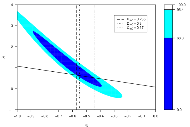
Figure 1: The current constraint on the plane $(q_{0},j_{0})$. The solid line is the relation $j_{0}(q_{0})$ fulfilled in the model. Additionally, for this relation the $1\sigma$ confidence level interval for $\Omega_{\text{m},0}$ is drawn.

We consider, for simplicity, the testing of the interaction for the flat model and the case $w_{X}=-1$ which corresponds the decaying cosmological constant. This allows to substitute $\nu\to w_{X}\nu$. On Fig. 1, from relation (21) with $w_{X}=-1$, the line $j_{0}=q_{0}+\frac{3}{2}(\Omega_{\text{m},0}-\nu)$ is drawn when we assume that baryonic matter $\Omega_{\text{m},0}-\nu$ is equal $0.05$. This relation allows us to estimate the interval on $\Omega_{\text{m},0}$ and $j_{0}$ on the $1\sigma$ confidence level. We mark the line $j_{0}(q_{0})$ and the vertical band to denote the interval with the $1\sigma$ confidence level for $q_{0}\in(-0.5725,-0.445)$ which gives $\Omega_{\text{m},0}\in(0.285,0.37)$. In this interval of $\Omega_{\text{m},0}$ the jerk $j_{0}$ is about $0.6$.

It is very interesting that present SNIa observations allowed us to measure the interaction without any special assumptions about physics of the transfer process. We thus determined the transfer energy parameter $\nu$ and concluded that if we assume that the Universe is flat then the energy transfer takes place from the dark energy to dark matter.

IV The energy transfer parameter from SNIa data

In the previous section it was considered that $\Omega_{\text{b},0}=\Omega_{\text{m},0}-\nu$. Now we turn to estimation of the energy transfer parameter $\nu$ using the SNIa data. It would be useful to consider two situation. First, the energy transfer is between decaying vacuum and matter sectors, and second, it is between the phantom ($p_{X}=4/3\rho_{X}$) and matter sectors. We would like to answer on two questions.

• What is the interval of $\Omega_{\text{m},0}$ which rules out the energy energy transfer ($\nu=0$) on the confidence level $95\%$?

• Is it possible to tell a scenario with energy transfer and another with variable $w_{X}$?

To answer to the first question we test the hypothesis that $\nu=0$. The transfer from decaying vacuum to matter sectors can be ruled out on the confidence level $95\%$ for $\Omega_{\text{m},0}\in(0.23,0.32)$ (Fig. 2), while the transfer from phantom to matter sectors is ruled out for $\Omega_{\text{m},0}\in(0.30,0.37)$ on the same confidence level (Fig. 3). Therefore the transfer between decaying vacuum and matter sector seems to be excluded because the extragalactic observations and CMB observations favor the values of $\Omega_{\text{m},0}$ in the obtained interval. On the other hand these other observations indicate that the transfer between phantom and matter sectors is possible. Hence if we have other arguments about phantom existence in the universe and if we accept that $\Omega_{\text{m},0}\simeq 0.27$ as indicated by WMAP measurements then the energy transfer is necessary.

Figure 2: The dependency of $\Omega_{\text{m},0}$ on $\nu$ for the transfer between decaying vacuum and matter sectors.

Figure 3: The dependency of $\Omega_{\text{m},0}$ on $\nu$ for the transfer between phantom and matter sectors.

Adopting the same analysis from the previous sections to the case of no energy and variable $w(z)=w_{0}+w_{1}z$ we obtain analogous formulas in which $\nu w_{0}$ is replaced by $w_{1}\Omega_{X,0}$. To answer the second question we analyze the Hubble diagram (Fig. 4). It is shown that for very distant supernovae ($z\simeq 2$) the model with variable $w(z)$ predicts the brighter supernovae.

Figure 4: The residuals in respect to the Einstein-de Sitter model (the base line) for the $\Lambda$CDM model (the upper line), the model with variable $w(z)$ (the middle line), and the model with transfer with best fitted $j_{0}=1.26$ and $q_{0}=-0.64$ (the lower line).