Cosmological Surprises from Braneworld models of Dark Energy
Abstract
Properties of Braneworld models of dark energy are reviewed. Braneworld models admit the following interesting possibilities: (i) The effective equation of state can be as well as . In the former case the expansion of the universe is well behaved at all times and the universe does not run into a future ‘Big Rip’ singularity which is usually encountered by Phantom models. (ii) For a class of Braneworld models the acceleration of the universe can be a transient phenomenon. In this case the current acceleration of the universe is sandwiched between two matter dominated epochs. Such a braneworld does not have a horizon in contrast to LCDM and most Quintessence models. (iii) For a specific set of parameter values the universe can either originate from, or end its existence in a Quiescent singularity, at which the density, pressure and Hubble parameter remain finite, while the deceleration parameter and all invariants of the Riemann tensor diverge to infinity within a finite interval of cosmic time. (iv) Braneworld models of dark energy can loiter at high redshifts: . The Hubble parameter decreases during the loitering epoch relative to its value in LCDM. As a result the age of the universe at loitering dramatically increases and this is expected to boost the formation of high redshift gravitationally bound systems such as black holes at and lower-mass black holes and/or Population III stars at , whose existence could be problematic within the LCDM scenario. (v) Braneworld models with a time-like extra dimension bounce at early times thereby avoiding the initial ‘Big Bang singularity’. (vi) Both Inflation and Dark Energy can be successfully unified within a single scheme (Quintessential Inflation).
Inter-University Centre for Astronomy and Astrophysics, Pune 411 007, India
1 Introduction
One of the most remarkable discoveries of the past decade is that the universe is accelerating. Evidence for an accelerating universe comes from observations of high redshift type Ia supernovae treated as standardized candles [1] and, more indirectly, by observations of the cosmic microwave background and galaxy clustering [2, 3]. Perhaps the simplest explanation for acceleration is the presence of vacuum energy exhibiting itself as a small cosmological constant with equation of state = constant. However, its un-evolving nature implies that the cosmological constant must be set to an extremely small value in order to dominate the expansion dynamics of the universe at precisely the present epoch and this gives rise (according to one’s perspective) either to an initial ‘fine-tuning’ problem or to a ‘cosmic coincidence’ problem. As a result several radically different alternative methods of generating ‘dark energy’ at a sufficiently late cosmological epoch have been suggested (see [4, 5, 6, 7, 8] for reviews on this subject). In this talk I will focus on one such approach which rests on the notion that space-time is higher-dimensional, and that our observable universe is a (3+1)-dimensional ‘brane’ which is embedded in a (4+1)-dimensional ‘bulk’ space-time. As we shall see, higher-dimensional braneworld models allow the expansion dynamics to be radically different from that predicted by conventional Einstein gravity in 3+1 dimensions. Some cosmological ‘surpises’ which spring from Braneworld models include:
-
•
Both early and late time acceleration can be successfully unified within a single scheme (Quintessential Inflation) in which the very same scalar field which drives Inflation at early times becomes Quintessence at late times.
-
•
The (effective) equation of state of dark energy in the braneworld scenario can be ‘phantom-like’ () or ‘Quintessence-like’ (). (These two possibilities are essentially related to the two distinct ways in which the brane can be embedded in the bulk.)
-
•
The acceleration of the universe can be a transient phenomenon: braneworld models accelerate during the present epoch but return to matter-dominated expansion at late times.
-
•
A class of braneworld models encounter a Quiescent future singularity, at which constant, but . The surprising feature of this singularity is that while the Hubble parameter, density and pressure remain finite, the deceleration parameter and all curvature invariants diverge as the singularity is approached.
-
•
A spatially flat Braneworld can mimick a closed universe and loiter at large redshifts.
-
•
A braneworld embedded in a five-dimensional space in which the extra (bulk) dimension is time-like can bounce at early times, thereby generically avoiding the big bang singularity. Cyclic models of the universe with successive expansion-contraction cycles can be constructed based on such a bouncing braneworld.
Let us now dwell a little on each of these cosmological properties (‘surprises’).
2 Quintessential Inflation on the Brane
An intriguing issue in cosmology is that the universe appears to accelerate twice: once at the very beginning during Inflation and again about 10 billion years later, during the present epoch. Although most theoretical models assume that there is no real connection between the two epochs and that Inflation and Dark energy are distinct physical entities, it might well be that the two phenomena are in fact related, and that the same scalar field which initially drives inflation, later, when its density has been considerably reduced, plays the role of Quintessence. This notion of Quintessential Inflation was first explored in the context of the Einstein gravity in 3+1 dimensions by Peebles and Vilenkin [11]. The possibility that Braneworld models could provide a more efficient realisation of this scenario was suggested by Copeland, Liddle and Lidsey [12] and subsequently discussed in greater detail by several authors [13, 14, 15, 16, 17].
The main line of reasoning behind this approach is simple. In the Randall–Sundrum model [9] the modified Einstein equations on the brane contain high-energy corrections as well as the projection of the Weyl tensor from the bulk on to the brane. The Friedmann equation on the brane in this case becomes [10]
| (1) |
where , is the brane tension, is the value of the cosmological constant in the five-dimensional ‘bulk’ and is the ‘dark radiation’ term which describes the projected five-dimensional degrees of freedom onto the brane. It is easy to see from (1) that
| (2) |
where
| (3) |
is the effective four dimensional cosmological constant in the Randall–Sundrum model.
During Inflation the expansion of the universe is driven by a scalar field propagating on the brane with energy density and pressure given by
| (4) |
while the evolution equation for the scalar field is
| (5) |
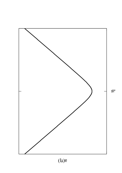
Braneworld models add an interesting new dimension to the scalar-field dynamics. As demonstrated by (1), for a quadratic density term appears in the modified Friedmann equation on the brane. This radically alters the expansion dynamics at early epochs by speeding up the rate of expansion and the value of the Hubble parameter, which now becomes instead of the more conventional . Since the value of affects the motion of through the damping term ‘’ in (5), the scalar field experiences significantly greater damping in braneworld cosmology than in conventional GR. Consequently, inflation on the brane can be realized by very steep potentials – precisely those that are used to describe Quintessence. The braneworld scenario therefore provides us with the opportunity to unify inflation and dark energy through the notion of quintessential inflation [11, 21, 12, 13, 14, 15, 17]. An example of quintessential inflation is shown in Figure 1.
An important property of Quintessential Inflation on the brane is that once the inflationary regime is over and braneworld corrections cease to play an important role, the extreme steepness of the potential causes the scalar field to plunge down its potential resulting in a ‘kinetic regime’ prior to reheating during which . It is well known that the spectrum of relic gravity waves created quantum mechanicaly during Inflation is sensitive to and bears an imprint of the post-inflationary equation of state [18, 19]. The effect of the kinetic regime is to create a ‘blue’ gravity wave spectrum on short wavelength scales which is an important observational signature of Quintessential Inflation on the brane [14, 17]; see also [20].

3 Braneworld models of Dark Energy with and
A radically different way of making the universe accelerate was suggested in [23, 27]. The braneworld model which I now discuss presents a successful synthesis of the higher-dimensional ansatzes proposed by Randall and Sundrum [9] and Dvali, Gabadadze, and Porrati [23], and is described by the action [24]
| (6) |
Here, is the scalar curvature of the five-dimensional metric in the bulk, and is the scalar curvature of the induced metric on the brane, where is the vector field of the inner unit normal to the brane. The quantity is the trace of the symmetric tensor of extrinsic curvature of the brane, and denotes the Lagrangian density of the four-dimensional matter fields whose dynamics is restricted to the brane (the notation and conventions are those of [25]). Integrations over the bulk and brane are taken with the natural volume elements and , respectively. The constants and denote, respectively, the five-dimensional and four-dimensional Planck masses, is the five-dimensional (bulk) cosmological constant, and is the brane tension.
An important difference between the action (6) and that describing the Randall–Sundrum cosmology is the presence of the term in (6). This term can be thought of as resulting from the backreaction of quantum fluctuations of matter fields residing on the brane, and this mechanism of generating the gravitational part of the action was proposed by Sakharov in a seminal paper in 1967 [26]. The effect of including such a term in the braneworld action was explored in [24, 23, 27].
Action (6) leads to the following expression for the Hubble parameter on the brane for a spatially flat universe [27]:
| (7) |
where
| (8) |
Note that the four-dimensional Planck mass is related to the effective Newton’s constant on the brane as . The two Planck masses and define a new length scale in a braneworld which begins to accelerate at the current epoch [23, 27]. (Other applications of braneworlds to the late-time acceleration of the universe are discussed in [29, 36, 30, 31, 33, 34, 35, 28].)
The two signs in (7) correspond to two branches of braneworld models and are related to the two different ways in which the brane can be embedded in the bulk. As shown in [27], the ‘’ sign in (7) corresponds to late time acceleration of the universe driven by dark energy with an ‘effective’ equation of state (we call this model BRANE2) whereas the ‘’ sign is associated with phantom-like behaviour (this model is called BRANE1).
Some limiting cases of (7) will be of interest to the reader:
- 1.
-
2.
In the other extreme case when , extra-dimensional effects become unimportant, and (7) reduces to the LCDM model
(9) - 3.
Consider now the Braneworld with the ‘’ sign on the right-hand side of (7), i.e. BRANE1. In this case the Hubble parameter on the brane can be rewritten as:
The term is composed of two terms, namely, a constant -term and a ‘screening term’:
| (10) |
Screening term
Since the screening term decreases with time, the value of the effective cosmological constant increases. Therefore the Braneworld behaves just like a Phantom model () but without Phantom’s problems: no violation of the weak energy condition and no future singularity. Indeed, from (3) its clear that the universe evolves to CDM in the future (see also [36, 40, 41, 37, 38, 39, 42, 43, 44] [45, 46, 47, 48, 49, 50, 51, 52, 53] for discussions of related issues).
The fact that the Braneworld model (7) can give rise to Phantom-like behaviour can also be seen if we rewrite (7) in terms of the cosmological redshift ‘z’ so that [27]
| (11) | |||||
where we have set the dark radiation term in (7) to zero () and
| (12) |
The quantities satisfy the constraint equation
| (13) |
where the sign in (13) is commensurate with that in (11). For future reference we also note the cosmological density associated with the four-dimensional cosmological constant (3) in Randall–Sundram cosmology
| (14) |
The expression for the current value of the effective equation of state is
| (15) |
and we immediately find that when we take the lower sign in (15), which corresponds to choosing one of two possible embeddings of this braneworld in the higher dimensional bulk (this is BRANE1). (The second choice of embedding (BRANE2) gives .) It is important to note that all BRANE1 models have and at . They therefore successfully cross the ‘great divide’ at (see page 26 of [27] for a discussion of this issue).
4 Transient Dark Energy
Braneworld cosmology has the interesting property that it allows the acceleration of the universe to be a transient phenomenon. (In [27] these models were referred to as ‘Disappearing Dark Energy’ (DDE).) Indeed, by setting the effective four dimensional cosmological constant (3) to zero so that in (14) we get
| (16) |
Selecting the lower sign in (16) and substituting in (11) we find that222Note that the case leads to transient acceleration with which is unrealistic [27].
| (17) |
which vanishes for the upper sign when . This implies that, since the effective four
dimensional cosmological constant vanishes,
the universe reverts to matter dominated
expansion in the future:
. The current acceleration of the
universe is therefore a transient phase in this model, as illustrated in
figure 2.

It is well known that an eternally accelerating universe is endowed with a cosmological event horizon which prevents the construction of a conventional S-matrix describing particle interactions within the framework of string or M-theory [54]. A transiently accelerating braneworld may therefore help reconcile string/M-theory with accelerating cosmology, which is an attractive feature of this braneworld cosmology.
5 Quiescent Future Singularity
As remarked earlier, an interesting property of the Braneworld (7) is that the late-time expansion of the universe can culminate in a ‘Quiescent’ singularity at which the density, pressure and Hubble parameter remain finite while the deceleration parameter and geometrical invariants constructed from the Riemann tensor diverge [55].
In order to appreciate the origin of such unusual future singularities in the braneworld, consider again the expansion law (11). For simplicity, we shall only discuss the solution corresponding to the ‘+’ sign in (11) (called BRANE2 in [27]).
A necessary and sufficient condition for the existence of a Quiescent singularity is for the inequality
| (18) |
to be satisfied [55]. In this case the expression under the square root of (11) becomes zero at a suitably late time, and the cosmological solution cannot be extended beyond this time. It can be shown that the scale factor and its first time derivative remain finite, while all the higher time derivatives of tend to infinity as the singularity is approached.

The limiting redshift, , at which the braneworld becomes singular is given by
| (19) |
The time of occurance of the singularity (measured from the present moment) can easily be determined from
| (20) |
where is given by (11). In Fig. 3 we show a specific braneworld model having , , . In keeping with observations of high redshift supernovae our model universe is currently accelerating [1], but will become singular at , i.e. after Gyr ( km/sec/Mpc). Figure 3 demonstrates that the deceleration parameter becomes singular as is approached:
| (21) |
while the Hubble parameter remains finite:
| (22) |
The possible presence of such ‘Quiescent’ singularity in Braneworld theory can also be seen from the following consideration. As shown in [27], the action (6) leads to the bulk being described by the usual Einstein equation with cosmological constant:
| (23) |
while the field equation on the brane is
| (24) |
Here, is the stress-energy tensor on the brane. A divergent form for the extrinsic curvature (underlined term) caused by a singular embedding of the brane in the bulk will, through (24), lead to a singular value for the Einstein tensor even though all components of the stress-energy tensor on the brane remain finite !
More generally it is well known that Quiescent singularites occur when the original equations of motion are non-linear with respect to the highest derivative. They have earlier been discussed in the context of Einstein gravity with the conformal anomaly [56]. (This result is not surprising in view of the formal similarity between braneworld theory and GR-based models with the conformal anomaly, discussed in [27].) ‘Determinant singularities’ having a similar structure and properties are known to arise in the anisotropic Bianchi I model containing a dilaton coupled to a Gauss–Bonnet term in the action [57] and also in other cosmological models [58, 59]. For instance [58] refer to singularities in which the deceleration parameter tends to infinity as the ‘Big Brake’ while in [59] they are called ‘sudden’ singularities (see also [60]).
We should also emphasise that both the past and future quiescent singularities occur for a wide range in parameter space and might provide an interesting alternative to the ‘big bang’/‘big crunch’ singularities of general relativity.
6 Loitering Braneworld Models

An interesting aspect of the Braneworld models (7) is that they allow for the existence of an early loitering epoch [61]. Loitering is characterized by the fact that the Hubble parameter dips in value over a narrow redshift range referred to as the ‘loitering epoch’. During loitering density perturbations are expected to grow rapidly. In addition, since the expansion of the universe slows down, its age near loitering dramatically increases. An early epoch of loitering is expected to boost the formation of high redshift gravitationally bound systems such as black holes at and lower-mass black holes and/or Population III stars at , whose existence could be problematic within the LCDM scenario.
To demonstrate the possibility of loitering note that for large values of the ‘dark radiation’ term , when and , equation (7) acquires the form
| (25) |
Equation (25) bears a formal resemblance to the Hubble parameter in standard GR
| (26) |
Remarkably, the role of the spatial curvature in (26) is played by the dark-radiation term in (25); consequently, a spatially open universe is mimicked by the BRANE2 model whereas a closed universe is mimicked by BRANE1.
Loitering solutions in standard cosmology were first found for a closed FRW model with a cosmological constant in [62]. Loitering in more general situations was discussed in [63, 64, 65, 61]. An intriguing aspect of braneworld models is that, since a spatially flat braneworld can behave dynamically just like a closed universe, loitering may be realised within a spatially flat setting and therefore be consistent both with Inflationary cosmology and recent CMB results [2]. Indeed, loitering solutions to (7) & (25) can easily be found by requiring that the loitering condition is satisfied. This allows us to determine the ‘loitering redshift’ [61]
| (27) |
From this expression we find that the universe will loiter at a large redshift provided . Since , loitering at large redshifts is not difficult to achieve.
One should note here that a closed FRW universe with a cosmological constant can loiter only at rather small redshifts: for [63]. Therefore Braneworld cosmology is endowed with two fundamentally new attributes: (i) it permits loitering in a spatially flat universe and (ii) it allows the loitering redshift to be large. Neither of these possibilities is allowed in standard Einsteinian cosmology.
The Hubble parameter at loitering is given by the approximate expression [61]
| (28) |
Examples of a loitering model are shown in Fig. 5, where the Hubble parameter of a universe which loitered at is plotted against the redshift. The right hand panel of figure 5 illustrates the fact that the loitering universe can show a variety of interesting behaviour: (i) top curve, is monotonically increasing and in the loitering interval; (ii) middle curve, appears to have an inflexion point () during loitering; (iii) lower curve, has both a maximum and a mininimum, the latter occuring in the loitering regime.

A loitering universe could have several important cosmological consequences, one of them being that the age of the universe during loitering increases, as shown in Fig. 6. The reason for the age increase rests in the expression
| (29) |
which shows that a lower value of close to loitering will boost the age of the universe at that epoch. An important consequence of having a larger age of the universe at (or so) is that astrophysical processes at these redshifts have more time in which to develop. This is especially important for gravitational instability which forms gravitationally bound systems from the extremely tiny fluctuations existing at the epoch of last scattering. Thus, an early loitering epoch may be conducive to the formation of Population III stars and low-mass black holes at and also of black holes at lower redshifts () whose existence could be problematic within the LCDM scenario [66]. (Note that age of a LCDM universe at is years for .)
Another important property of a loitering universe is that it can alter the reionization properties of the inter-galactic medium at moderate redshifts . One should note in this context that a major surprise emerging from the WMAP experiment was the discovery of a large optical depth to reionization [2], which, when translated within the framework of LCDM (assuming instantaneous reionization), implies a rather early epoch for reionization .
In order to appreciate how loitering might alter these conclusions consider the following expression for the optical depth to a redshift
| (30) |
where is the electron density and is the Thompson cross-section describing scattering between electrons and CMB photons. During loitering drops below its value in LCDM, therefore . For instance the redshift of reionization drops to for the loitering models shown in figure 5. Loitering decreases the redshift of reionization and increases the age of the universe thereby alleviating the existing tension between the high redshift universe and dark energy cosmology [61].
6.1 The effective equation of state in a loitering Braneworld.
The deceleration parameter and the effective equation of state in our loitering model are given by the expressions
| (31) |
where is determined from (11). The current values of these quantities are
| (32) |
where . From Eq. (32) we find that if ; in other words, our loitering universe has a phantom-like effective equation of state (EOS). (In particular, for the loitering models shown in Fig. 5, we have , , (top to bottom), all of which are in excellent agreement with recent observations [67, 68].)
An interesting consequence of the loitering braneworld is that the matter density exceeds unity at some time in the past. This follows immediately from the fact that, since the value of in the loitering braneworld model is smaller than its counterpart in LCDM, the value of is larger than its counterpart in LCDM. One important consequence of this behaviour is that, as expected from (32), the effective equation of state (EOS) blows up precisely when .

In Fig. 7, we show that, in contrast to the singular behaviour of the EOS, the deceleration parameter remains finite and well behaved even as . Note that the finite behaviour of when reflects the fact that the EOS for the braneworld is an effective quantity and not a real physical property of the theory. This is an important point with broader ramifications since it concerns dark energy models constructed from modifications to the ‘gravity sector’ of the theory of which Braneworld models are but one example (others being: scalar-tensor gravity, Cardassian approximation, gravity, k-essence, to name but a few). Let me therefore dwell on this point in some more detail.
Within the framework of general relativity the rate of expansion of a FRW universe and its acceleration are described by the pair of equations
| (33) |
where the summation is over all matter fields contributing to the dynamics of the universe. Within this framework, and in the absence of spatial curvature, the energy density and pressure of dark energy can be defined as:
| (34) |
where is the critical density associated with a FRW universe and is the deceleration parameter. An important consequence of using (6.1) & (6.1) is that the ratio can be expressed in terms of the deceleration parameter
| (35) |
i.e. we recover equation (31) which had earlier been used to determine the equation of state in a loitering universe. Since this derivation of uses the general relativistic formulation it can be expected to recover standard results for GR-based dark energy models such as LCDM and quintessence. However the same cannot be said of braneworld models since the Hubble parameter for the latter contains interaction terms between matter and dark energy (see for instance equation (11)) and therefore does not subscribe to the general relativistic format (6.1). “One can however extend the above definition of to non-Einsteinian theories by defining dark energy density to be the remainder term after one subtracts the matter density from the critical density in the Einstein equations. It should be emphasised that, according to this prescription all interaction terms between matter and dark energy (such terms arise in scalar-tensor and brane models) are attributed solely to dark energy. Therefore defined according to (35) is an effective equation of state in these models and not a fundamental physical entity (as it is in LCDM, for instance)” [69]. The fact that the EOS is indeed an effective equation of state and not a fundamental physical quantity is illustrated by figure 7 which shows that diverges when and that this divergence is not reflected in other characteristics of expansion such as the deceleration parameter. 333It should also be stressed that the propagation velocity of small inhomogeneities in dark energy is generically neither , nor . Therefore although is an important physical quantity it does not provide us with an exhaustive description of dark energy and its use as a diagnostic should be treated with some caution, as emphasised in [69].
6.2 The Statefinder diagnostic and Dark Energy
As demonstrated above, the equation of state is not a fundamental physical quantity for dark energy models based either on non-Einsteinian gravity (scalar-tensor theories, Cardassian approximation, k-essence, R + f(R) gravity, etc.) or on Einstein gravity in more than 3+1 dimensions, or indeed in cosmological models with explicit interaction terms between dark matter and dark energy. In all these cases it is useful to supplement the effective equation of state by other geometrical variables, which are ‘model independent’, in the sense that they do not depend upon an underlying theory of gravity in an explicit way, but can be constructed solely from the expansion factor and its derivatives, and therefore would be expected to apply to all metric theories of gravity defined on a space-time manifold. In all such theories the universe can be expected to be characterised by the following general form for the expansion factor:
| (36) |
Usually dark energy models such as quiessence, quintessence, k-essence, braneworld models, Chaplygin gas etc. give rise to families of curves having quite different properties. Since we know that the acceleration of the universe is a fairly recent phenomenon we can, in principle, confine our attention to small values of in (36).
Accordingly, as dicussed in [70, 69], a new diagnostic of dark energy called ‘statefinder’ can be constructed using both the second and third derivatives of the expansion factor (see also [72, 73, 74]). The statefinder pair , defines two new cosmological parameters (in addition to and ):
| (37) | |||||
| (38) |
In figure 8 we show the statefinder pair for several dark energy models including LCDM, quintessence and the Chaplygin gas. For the sake of completeness we say a few words about each of these models below. (Note that the ensuing discussion is largely based on [70, 69] and the reader should refer to these papers for more details.)

-
•
In Quiessence the equation of state of dark energy is a constant so that
(39) where = constant. Important examples of quiessence include: LCDM (), a network of non-interacting cosmic strings (), domain walls () and phantom models (). Quiessence in a FRW universe can also be produced by a scalar field (quintessence) which has the potential , with appropriately chosen values of and [4, 71, 70].
-
•
The density and pressure of Quintessence are given by
(40) while evolution of the Quintessence field is governed by the equation of motion
(41) where
(42) It is clear from (40) that provided . Models with this property can lead to an accelerating universe at late times. An important subclass of Quintessence models displays the so-called ‘tracker’ behaviour during which the ratio of the scalar field energy density to that of the matter/radiation background changes very slowly over a substantial period of time. Models belonging to this class satisfy and approach a common evolutionary ‘tracker path’ from a wide range of initial conditions.
-
•
An interesting alternative form of dark energy is provided by the Chaplygin gas [75, 76] which obeys the equation of state
(43) The energy density of the Chaplygin gas evolves according to
(44) from where we see that as and as . Thus, the Chaplygin gas behaves like pressureless dust at early times and like a cosmological constant during very late times.
The Hubble parameter for a universe containing cold dark matter and the Chaplygin gas is given by
(45) where . It is easy to see from (45) that
(46) Thus, defines the ratio between CDM and the Chaplygin gas energy densities at the commencement of the matter-dominated stage.
For all of the above models the statefinders and can be easily expressed in terms of the Hubble parameter and its derivatives as follows:
| (47) |
where and is given by (39), (42), (45), (11) for the different dark energy models. The results, shown in figures 8 & 9, demonstrate that the Statefinder diagnostic can successfully differentiate between dark energy models as diverse as LCDM, Quintessence, the Chaplgyn Gas and Braneworlds (see [77] for other recent applications of the Statefinder diagnostic).
7 Bouncing Braneworlds
A remarkable feature of Braneworld cosmology is that the expansion dynamics of the early universe can be non-singular. Indeed, as shown in [78] bouncing Braneworld models can be constructed, based upon a Randall–Sundrum type action, but in which the extra dimension is time-like. In this case one starts from the action [78]
| (48) |
where the parameter if the signature of the bulk space is Lorentzian, so that the extra dimension is spacelike, and if the signature is , so that the extra dimension is timelike. The evolution equations resulting from (48) have the form [78]
| (49) |
Where is the effective gravitational constant, and is the effective cosmological constant on the brane. For , Eq. (49) reduces to the well-known Randall–Sundrum form (we ignore and which are unimportant for our purposes)
| (50) |
On the other hand if then we obtain
| (51) |
where the brane tension . (The two braneworld models (50) and (51) are dual, as demonstrated in [79].) Equation (51) clearly demonstrates that when i.e. the universe bounces when the energy density of matter becomes sufficiently large. It is important to note that the singularity-free nature of the early universe is a generic outcome of this theory and does not depend upon whether or not matter violates the energy conditions. An example of a bouncing braneworld universe is shown in figure (10) below.
An early time bounce, such as (51), can be used to construct cyclic models of the universe [80, 81, 82, 83]. Consider for instance the mechanism proposed in [80] in which Phantom dark energy is presumed to exist in addition to matter and radiation so that
| (52) |
where , , and in the case of Phantom leading to
| (53) |
It is clear from (53) that grows at small as well as large values of . Indeed within one cycle the value of will pass through zero twice: (i) at early times when the bounce in (51) is brought about due to large values of the radiation density and (ii) during late times, when the large value of the Phantom energy leads to in (51) and initiates the universe’s recollapse.
Similarly, it is easy to show that a bouncing spatially closed universe with matter satisfying will also be ‘cyclic’ in the sense that it will pass through an infinite number of nonsingular expanding-collapsing epochs [81, 82]. As demonstrated in [81, 82], a massive scalar field in such a universe usually leads to an increase in the amplitude of consecutive expansion cycles and to a gradual amelioration of the flatness problem; see figure 11.

8 Conclusions
Braneworld models hold interesting consequences both for the early as well as the late-time evolution of the universe. At early times, the increased rate of expansion in RSII type braneworlds allows scalar fields with steep potentials to play the dual role of being the inflaton as well as Quintessence.
Braneworld models in which the RSII action is supplemented by an induced gravity term on the brane have important consequences for the late-time evolution of the universe. For instance: (i) The effective equation of state of dark energy in this scenario can be as well as . (ii) The current acceleration of the universe can be a transient phenomenon. (iii) The braneworld universe can end its existence in a Quiescent singularity at which the density, pressure and Hubble parameter remain finite, while the deceleration parameter and all invariants of the Riemann tensor diverge. (iv) Braneworld models of dark energy can loiter at high redshifts: . The Hubble parameter decreases during the loitering epoch relative to its value in LCDM. As a result the age of the universe at loitering dramatically increases and this is expected to boost the formation of high redshift gravitationally bound systems such as black holes at and lower-mass black holes and/or Population III stars at , whose existence could be problematic within the LCDM scenario. (v) In addition to the above, an RSII type Braneworld in which the extra dimension is time-like (instead of space-like) avoids the initial Big Bang singularity by bouncing at early times. This property (which holds even if matter satisfies all the energy conditions) has been used to construct cyclic models of a singularity free universe.
9 Acknowldgements
It is a pleasure to thank Yuri Shtanov who collaborated with me on most of the projects discussed in this paper.
References
- [1] S.J. Perlmutter et al., Astroph. J. 517, 565 (1999) [astro-ph/9812133]; A. Riess et al., Astron. J. 116, 1009 (1998) [astro-ph/9805201]. A.G. Riess, et al., Astroph. J. 607, 665 (2004) [astro-ph/0402512]
- [2] D.N. Spergel, et al., Phys. Rev. D 69, 103501 (2004) [astro-ph/0302209].
- [3] M. Tegmark, et al., astro-ph/0310723.
- [4] V. Sahni and A.A. Starobinsky, IJMP D 9, 373 (2000) [astro-ph/9904398].
- [5] S.M. Carroll, Living Rev.Rel. 4 1 (2001) [astro-ph/0004075].
- [6] P.J.E. Peebles and B. Ratra, Rev.Mod.Phys. 75, 559 (2002) [astro-ph/0207347].
- [7] T. Padmanabhan, Phys. Rep. 380, 235 (2003) [hep-th/0212290].
- [8] V. Sahni, Dark Matter and Dark Energy, Lectures given at the 2nd Aegean Summer School on the Early Universe, Ermoupoli, Island of Syros, Greece, astro-ph/0403324 .
- [9] L. Randall and R. Sundrum, Phys. Rev. Lett. 83, 3370 (1999), [hep-ph/9905221]; L. Randall and R. Sundrum, Phys. Rev. Lett. 83, 4690 (1999), [hep-th/9906064].
- [10] P. Binétruy, C. Deffayet, and D. Langlois, Nucl. Phys. B 565, 269 (2000), [hep-th/9905012]; C. Csáki, M. Graesser, C. Kolda, and J. Terning, Phys. Lett. B 462, 34 (1999), [hep-ph/9906513]; J. M. Cline, C. Grojean, and G. Servant, Phys. Rev. Lett. 83, 4245 (1999), [hep-ph/9906523]; P. Binétruy, C. Deffayet, U. Ellwanger, and D. Langlois, Phys. Lett. B 477, 285 (2000), [hep-th/9910219]. T. Shiromizu, K. Maeda, and M. Sasaki, Phys. Rev. D 62, 024012 (2001), [hep-th/9910076].
- [11] P. J. Peebles and A. Vilenkin, Phys. Rev. D 59, 063505 (1999).
- [12] E.J. Copeland, A. R. Liddle and J. E. Lidsey, Phys. Rev. D 64, 023509 (2001) [astro-ph/0006421].
- [13] G. Huey and Lidsey, Phys. Lett. B 514, 217 (2001).
- [14] V. Sahni, M. Sami and T. Souradeep, Phys. Rev. D65, 023518 (2002).
- [15] A. S. Majumdar, Phys.Rev. D64, 083503 (2001).
- [16] S. Nojiri and S. D. Odintsov, Phys. Rev. D 68, 123512 (2003); Phys. Lett. B 599, 137 (2004).
- [17] M. Sami and V. Sahni, Phys.Rev. D70, 083513 (2004).
- [18] A. A. Starobinsky, JETP Lett., 30, 682 (1979).
- [19] V. Sahni, Phys. Rev. D 42, 453 (1990).
- [20] M. Giovannini, Phys. Rev. D 58, 083504 (1998); Phys. Rev. D 60, 123511 (1999).
- [21] R. Maartens, D. Wands, B.A. Bassett and I.P.C. heard, Phys. Rev. D 62, 041301(R) (2000)
- [22] V. Sahni, and L. Wang, Phys. Rev. D 62, 103517 (2000).
- [23] G. Dvali, G. Gabadadze, and M. Porrati, Phys. Lett. B 485, 208 (2000), [hep-th/0005016].
- [24] H. Collins and B. Holdom, Phys. Rev. D 62, 105009 (2000), hep-ph/0003173; Yu. V. Shtanov, On Brane World Cosmology, hep-th/0005193; C. Deffayet, Phys. Lett. B 502, 199 (2001), hep-th/0010186.
- [25] R. M. Wald, General Relativity, University of Chicago Press, Chicago (1984).
- [26] A. D. Sakharov, Dokl. Akad. Nauk SSSR. Ser. Fiz. 177, 70 (1967) [Sov. Phys. Dokl. 12, 1040 (1968)]; reprinted in: Usp. Fiz. Nauk 161, 64 (1991) [Sov. Phys. Usp. 34, 394 (1991)]; Gen. Rel. Grav. 32, 365 (2000).
- [27] V. Sahni and Yu. V. Shtanov, JCAP 0311, 014 (2003), [astro-ph/0202346]; IJMP D 11, 1515 (2002), [gr-qc/0205111]; U. Alam and V. Sahni, Supernova Constraints on Braneworld Dark Energy, astro-ph/0209443.
- [28] J.S. Alcaniz, D. Jain, A. Dev Phys. Rev. D 66, 067301 (2002) [astro-ph/0206448]; D. Jain, A. Dev, J.S. Alcaniz Phys. Rev. D 66, 083511 (2002) [astro-ph/0206224]
- [29] K. Maeda, S. Mizuno, T. Torii Phys. Rev. D 68, 024033 (2003) [gr-qc/0303039].
- [30] R. Maartens Living Rev.Rel. 7, 7 (2004) [gr-qc/0312059].
- [31] P. Brax, C. van de Bruck, A-C. Davis, Rept.Prog.Phys. 67, 2183 (2004) [hep-th/0404011].
- [32] J.A.S. Lima, Braz.J.Phys. 34, 194 (2004) [astro-ph/0402109].
- [33] R. G. Vishwakarma and P. Singh, Class.Quant.Grav. 20, 2033 (2003) [astro-ph/0211285].
- [34] J.A. Alcaniz and N. Pires, Phys. Rev. D 70, 047303 (2004) [astro-ph/0404146].
- [35] A. Padilla, Infra-red modification of gravity from asymmetric branes, hep-th/0410033; A. Padilla, Cosmic acceleration from asymmetric branes, hep-th/0406157.
- [36] A. Lue and G.D. Starkmann, Phys. Rev. D D70, 101501 (2004) [astro-ph/0408246].
- [37] R. R. Caldwell, Phys. Lett. B 545, 23 (2002) [astro-ph/9908168].
- [38] J.M. Cline, S. Jeon and G.D. Moore, Phys. Rev. D 70, 043543 (2004) [hep-ph/0311312].
- [39] A.A. Starobinsky, JETP Lett. 68, 757 (1998).
- [40] T. Chiba, T. Okabe, T. and M. Yamaguchi, Phys. Rev. D 62, 023511 (2000).
- [41] S. Hellerman, N. Kaloper and L. Susskind, JHEP 0106:003,2001 [hep-th/0104180].
- [42] B. McInnes, JHEP 0208, 029 (2002) [hep-th/0112066].
- [43] R.R. Caldwell, M. Kamionkowski and N.N. Weinberg, Phys.Rev.Lett. 91, 071301 (2003) [astro-ph/0302506].
- [44] S.M. Carroll, M. Hoffman and M. Trodden, Phys. Rev. D 68, 023509 (2003) [astro-ph/0301273].
- [45] P. Frampton, Phys. Lett. B 555, 139 (2003).
- [46] P. Frampton and T. Takahashi, Phys. Lett. B 557, 135 (2003).
- [47] P. Singh, M. Sami and N.K. Dadhich Phys. Rev. D 68, 023522 (2003) [hep-th/0305110].
- [48] V.B. Johri, Phys. Rev. D 70, 041303 (2004) [astro-ph/0311293].
- [49] M. P. Dabrowski, T. Stachowiak, M. Szydlowski, Phys. Rev. D 68, 103519 (2003) [hep-th/0307128];
- [50] S. Nojiri and S. D. Odintsov, Phys. Lett. B 595, 1 (2004), hep-th/0405078; S. Nojiri and S. D. Odintsov, The final state and thermodynamics of dark energy universe, hep-th/0408170; M. C. B. Abdalla, S. Nojiri, and S. D. Odintsov, Consistent modified gravity: dark energy, acceleration and the absence of cosmic doomsday, hep-th/0409177.
- [51] S. Nesseris, L. Perivolaropoulos Phys. Rev. D 70, 123529 (2004) [astro-ph/0410309].
- [52] C. Csaki, N. Kaloper and J. Terning, Exorcising , astro-ph/0409596.
- [53] S.K. Srivastava, Future Universe With Without Big Smash, astro-ph/0407048.
- [54] W. Fischler, A. Kashani-Poor, R. McNees, and S. Paban, JHEP 0107, 3 (2001) [hep-th/0104181]; J. Ellis, N. E. Mavromatos, and D. V. Nanopoulos, String theory and an accelerating universe, hep-th/0105206; J. M. Cline, JHEP 0108, 35 (2001) [hep-ph/0105251]; X.-G. He, Accelerating universe and event horizon, astro-ph/0105005.
- [55] Yu. Shtanov and V. Sahni, Class.Quant.Grav. 19, L101 (2002) [gr-qc/0204040].
- [56] R. M. Wald, Ann. Phys. 110, 472 (1978); M. V. Fischetti, J. B. Hartle, and B. L. Hu, Phys. Rev. D 20, 1757 (1979).
- [57] S. Alexeyev, A. Toporensky, and V. Ustiansky, Phys. Let. B 509, 151 (2001); A. Toporensky and S. Tsujikawa, Phys. Rev. D 65, 123509, (2002), [gr-qc/0202067].
- [58] V. Gorini, A. Yu. Kamenshchik, U. Moschella, V. Pasquier, Phys. Rev. D 69, 123512 (2004).
- [59] J.D. Barrow, Class.Quant.Grav. 21, L79 (2004).
- [60] S. Cotsakis, I. Klaoudatou, Future Singularities of Isotropic Cosmologies, gr-qc/0409022.
- [61] V. Sahni and Yu. Shtanov, astro-ph/0410221.
- [62] A. G. Lemaître, MNRAS 91, 483 (1931).
- [63] V. Sahni, H. Feldman and A. Stebbins, Astrophys. J. 385, 1 (1992).
- [64] S. Alexander, R. Brandenberger, D. Easson, Phys. Rev. D 62, 103509 (2000); R. Brandenberger, D. Easson, D. Kimberley, Nuc. Phys. B623, 421 (2002).
- [65] M. Chevallier and D. Polarski, Int. J. Mod. Phys. D10, 213 (2001) [gr-qc/0009008]
- [66] G. T. Richards et al., Astron. J. 127, 1305 (2004) [astro-ph/0309274]; Z. Haiman and E. Quataert, The Formation and Evolution of the First Massive Black Holes, astro-ph/0403225; D. N. Spergel, et al., Astrophys. J. Suppl. 148, 175 (2003) [astro-ph/0302209]; R. Barkana and A. Loeb, In the Beginning: The First Sources of Light and the Reionization of the Universe, astro-ph/0010468; B. Ciardi and A. Ferrara, The First Cosmic Structures and their Effects, astro-ph/0409018.
- [67] U. Alam, V. Sahni, and A. A. Starobinsky, JCAP 06, 008 (2004), [astro-ph/0403687].
- [68] U. Seljak et al., Cosmological parameter analysis including SDSS Ly-alpha forest and galaxy bias: constraints on the primordial spectrum of fluctuations, neutrino mass, and dark energy, astro-ph/0407372.
- [69] U. Alam, V. Sahni, T. D. Saini and A. A. Starobinsky, MNRAS 344, 1057 (2003), [astro-ph/0303009].
- [70] V. Sahni, T.D. Saini, A.A. Starobinsky, and U. Alam, JETP Lett. 77 201 (2003) [astro-ph/0201498].
- [71] L.A. Urena-Lopez, T. Matos, Phys. Rev. D 62, 081302, (2000) [astro-ph/0003364].
- [72] T. Chiba and N. Nakamura, Prog. Theor. Phys. 100, 1077 (1998).
- [73] M. Visser, Class.Quant.Grav. 21, 2603 (2004) [gr-qc/0309109].
- [74] E. Linder, astro-ph/0404032.
- [75] A. Kamenshchik, U. Moschella, and V. Pasquier, Phys. Lett. B 511 265 (2001).
- [76] M.C. Bento, O. Bertolami, A.A. Sen, Phys. Rev. D D66, 043507 (2002) [gr-qc/0202064 ]; N. Bilic, G.B. Tupper and R. Viollier Phys. Lett. B 535, 17 (2002). J.S. Fabris, S.V. Goncalves and P.E. de Souza, astro-ph/0207430; V. Gorini, A. Kamenshchikand U. Moschella, Phys. Rev. D 67 063509 (2003) [astro-ph/0209395]; J.S. Alcaniz, D. Jain and A. Dev Phys. Rev. D 67, 043514 (2003) [astro-ph/0210476]; C. Avelino, L.M.G. Beca, J.P.M. de Carvalho, C.J.A.P. Martins, and P. Pinto, Phys. Rev. D 67, 023511 (2003) [astro-ph/0208528]; O. Bertolami, A.A. Sen, S. Sen and P.T. Silva, MNRAS 353, 329 (2004) [astro-ph/0402387].
- [77] W. Zimdahl and D. Pavon, Gen.Rel.Grav. 36, 1483 (2004) [gr-qc/0311067]; A.K.D. Evans, I.K. Wehus, O. Gron, O. Elgaroy astro-ph/0406407.
- [78] Yu. Shtanov and V. Sahni, Phys.Lett.B 557, 1 (2003) [gr-qc/0208047]
- [79] E. J. Copeland, S-J. Lee, J. E. Lidsey, S. Mizuno, astro-ph/0410110
- [80] M. G. Brown, K. Freese, W. H. Kinney, astro-ph/0405353
- [81] N. Kanekar, V. Sahni and Yu. Shtanov, Phys. Rev. D 63, 083520 (2001) [astro-ph/0101448].
- [82] Y-S. Piao, gr-qc/0407027
- [83] Y-S. Piao, Phys. Rev. D 70, 101302, (2004) [hep-th/0407258].