Massive galaxies & EROs at $z=1-3$ in cosmological hydrodynamic simulations: near-IR properties

Abstract

Recent observations have revealed a population of red massive galaxies at high redshift which are challenging to explain in hierarchical galaxy formation models. We analyze this “massive galaxy problem” with two different types of hydrodynamic simulations – Eulerian total variation diminishing (TVD) and smoothed particle hydrodynamics (SPH) — of a concordance $\Lambda$ cold dark matter ($\Lambda$CDM) universe. We consider two separate but connected aspects of the problem posed by these extremely red objects (EROs): (1) the mass-scale of these galaxies, and (2) their red colors. We perform spectrophotometric analyses of simulated galaxies in $B,z,R,I,J_{s},K_{s},K$ filters, and compare their near-infrared (IR) properties with observations at redshift $z=1-3$. We find that the simulated galaxies brighter than the magnitude limit of $K_{\rm vega}=20$ mag have stellar masses $M_{\star}\gtrsim 10^{11}{h^{-1}}{{\rm M}_{\odot}}$ and a number density of a few $\times 10^{-4}h^{3}{\rm\,Mpc}^{-3}$ at $z\sim 2$, in good agreement with the observed number density in the K20 survey. Therefore, our hydrodynamic simulations do not exhibit the “mass-scale problem”. The answer to the “redness problem” is less clear because of our poor knowledge of the amount of dust extinction in EROs and the uncertain fraction of star-forming EROs. However, our simulations can account for the observed comoving number density of $\sim 1\times 10^{-4}\,{\rm\,Mpc}^{-3}$ at $z=1-2$ if we assume a uniform extinction of $E(B-V)=0.4$ for the entire population of simulated galaxies. Upcoming observations of the thermal emission of dust in 24 $\mu$m by the Spitzer Space Telescope will help to better estimate the dust content of EROs at $z=1-3$, and thus to further constrain the star formation history of the Universe, and theoretical models of galaxy formation.

1 Introduction

Multiband photometry including the near infrared (IR) band makes it possible to estimate the stellar mass of high redshift galaxies when the observed photometric results are fitted with artificial galaxy spectra generated by a population synthesis model. Working in the near-IR also allows one to construct a mass-selected sample, because near-IR band emission is less affected by dust extinction than at shorter wavelengths and closely traces the total stellar mass. Using this technique, a number of recent observational studies have revealed a seemingly new population of very red, massive galaxies at redshift $z=1-3$ (e.g. Franx et al., 2003; Rudnick et al., 2003; Glazebrook et al., 2004; McCarthy et al., 2004; Fontana et al., 2004; Saracco et al., 2004, 2005; Daddi et al., 2004a, b; Cimatti et al., 2004).

In this paper, we first give a brief review of the results of some of the major surveys that detected such a population of galaxies (see Section 2). All of these recent observational studies, particularly at $z=1-3$, both in the UV and near-IR wavelengths, imply a range of novel tests for the hierarchical structure formation theory. We now face the important question as to whether this evidence for high-redshift massive galaxy formation is consistent with theoretical predictions based on the concordance $\Lambda$CDM model. This question is sometimes called the “massive galaxy problem”.

In more detail, the “massive galaxy problem” that is posed by these observations can be divided into two separate but connected issues: (1) the “mass-scale problem”, and (2) the “redness problem”. The first aspect asks whether the hierarchical CDM model can produce a sufficient number of massive galaxies by $z=1-2$. The second part of the problem, which seems to be more challenging for models, is whether there are enough very red, old, quiet, and massive galaxies. For example, Somerville et al. (2004) compared the results of the Great Observatories Origins Deep Survey (GOODS) data and the semi-analytic model of Somerville et al. (2001), and concluded that the semi-analytic model shows a deficit of both EROs and galaxies with $K<22$ at $z>1.5$, and that new or modified physics not yet accounted for in the semi-analytic models is needed to resolved this discrepancy. Therefore, it is of considerable interest whether hydrodynamic simulations of galaxy formation also suffer from the same problems.

In our first paper of the series (Nagamine et al., 2004), we argued that, based on two different types of hydrodynamic simulations (Eulerian TVD and SPH) and the theoretical model of Hernquist & Springel (2003) (hereafter H&S model), the predicted cosmic star formation rate (SFR) density peaks at $z\geq 5$, with a higher stellar mass density at $z=3$ than suggested by current observations, in contrast to some claims to the contrary. This star formation history predicts that 70 (50, 30)% of the total stellar mass at $z=0$ has already been formed by $z=1$ (2, 3). We also compared our results with those from the updated semi-analytic models of Somerville et al. (2001), Granato et al. (2000), and Menci et al. (2002), and found that our simulations and the H&S model predicts an earlier peak of the SFR density and a faster build-up of stellar mass density compared to these semi-analytic models.

It is then interesting to examine what our simulations predict for the properties of massive galaxies at $z\sim 2$. In our second paper (Nagamine et al., 2005), we analyzed for this purpose the same set of hydrodynamic simulations, focusing on the UV properties of the most massive galaxies at the relevant epochs. Using the latest population synthesis model of Bruzual & Charlot (2003), we computed the spectra of simulated galaxies and performed a spectrophotometric analysis in the $U_{n},G,R$ filter set. We found that the simulated galaxies at $z=2$ satisfy the color-selection criteria proposed by Adelberger et al. (2004) and Steidel et al. (2004) when we assume a Calzetti extinction with $E(B-V)\sim 0.15$. The total number density of simulated galaxies brighter than $R=25.5$ at $z=2$ was about $1\times 10^{-2}\,h^{3}\,{\rm Mpc}^{-3}$ for a uniform extinction of $E(B-V)=0.15$ (see Section 6 for a discussion of the number density of UV and IR selected galaxies). The most massive galaxies at $z=2$ have stellar masses $\geq 10^{11-12}{\rm M}_{\odot}$, and they typically have been continuously forming stars with a rate exceeding $30\,{\rm M}_{\odot}\,{\rm yr}^{-1}$ over a few Gyrs from $z=10$ to $z=2$, together with a significant number of starbursts reaching $1000\,{\rm M}_{\odot}\,{\rm yr}^{-1}$, often lasting for a few tens of million years, superposed on the continuous component. TVD simulations indicated a more sporadic star formation history than the SPH simulations. Those galaxies that appear to be red, passive systems at $z=2$ have completed the build-up of their stellar mass by $z\sim 3$, and have been quiet between $z=3$ and $z=2$. We argued that our results imply that hierarchical galaxy formation can account for the massive galaxies at $z\geq 1$.

In this paper, we extend our analysis to the near-IR properties of massive galaxies at $z=1-3$, with special focus on colors and stellar masses of galaxies. The paper is organized as follows. In Section 2, we give a brief summary of the current observational situation with respect to EROs, and in Section 3 we describe the simulations we use. In Section 4, we review our method for computing spectra and photometric magnitudes of simulated galaxies. We present our results for the near-IR properties of galaxies in Section 5. Finally, we summarize and discuss the implications of our work in Section 6.

2 Observational data on massive galaxies and EROs

The Gemini Deep Deep Survey (GDDS, Abraham et al., 2004) has obtained 225 secure spectroscopic redshifts of the reddest and most luminous galaxies with $K_{\rm vega}<20.6$ mag. These galaxies lie near the $I-K$ versus $I$ color-magnitude track mapped out by passively evolving galaxies in the redshift interval $0.8<z<2$, probing the ‘redshift desert’. The infrared selection means that the GDDS is observing not only star-forming galaxies, as in most high-redshift galaxy surveys, but also quiescent evolved galaxies. About 25% of their sample shows clear spectral signatures of evolved (pure old, or old + intermediate-age) stellar populations, 35% shows features consistent with either a pure intermediate-age or a young + intermediate-age stellar population. About 29% of the galaxies in the GDDS at $0.8<z<2$ are young starbursts with strong interstellar lines. Using the GDDS data, Glazebrook et al. (2004) estimated the stellar masses, and argued that there are a number of very massive, evolved red ($(I-K)_{\rm vega}>4$) galaxies with stellar masses $M_{\star}>10^{11}M_{\odot}$ at $z\sim 2$, which make a large contribution (30%) to the stellar mass density in the Universe. McCarthy et al. (2004) estimated the ages of the red galaxies at $1.3<z<2.2$ in the GDDS data, and found that they have a median age of $1-3$ Gyrs with a history of a strong starburst phase ($300-500\,{\rm M}_{\odot}\,{\rm yr}^{-1}$) in the past. These results suggest an early and rapid formation of massive galaxies at $z\gtrsim 1$.

Similarly, the recently completed K20 survey (e.g., Cimatti et al., 2002a, b, c) identified a sample of over 500 spectroscopic galaxies with $K_{s,\rm vega}<20$ with high spectroscopic completeness. Among these, $\sim 30$ galaxies had spectroscopic redshifts $z>1.4$. They also obtained $BVRIzJHK$ photometric data. Using the K20 data, Fontana et al. (2004) demonstrated that there are galaxies with stellar masses $M_{\star}>10^{11}{\rm M}_{\odot}$ at $z\simeq 2$. Cimatti et al. (2002c) showed that some semi-analytic models of galaxy formation underpredict the $K$ -band number counts compared to the K20 survey data, and suggested a possible problem with current semi-analytic models. Daddi et al. (2004a, b) identified a significant population of $z=2$ galaxies with $K_{s,{\rm vega}}<20$ with high average star formation rates of $SFR\sim 200\,{\rm M}_{\odot}\,{\rm yr}^{-1}$ and median extinctions of $E(B-V)\sim 0.4$. These values are significantly higher than those of Lyman break galaxies’ (LBGs’) ($SFR\sim 40\,{\rm M}_{\odot}\,{\rm yr}^{-1}$ and $E(B-V)\sim 0.15$). Cimatti et al. (2004) found 4 old, fully assembled, massive ($M_{\star}>10^{11}{\rm M}_{\odot}$) spheroidal galaxies at $1.6<z<1.9$ in the K20 data. The number density of such objects amounts to a few $\times 10^{-4}\,h^{3}\,{\rm\,Mpc}^{-3}$. In parallel to the K20 survey, Saracco et al. (2005) discovered 7 bright ($17.8<K_{\rm vega}<18.4$) massive evolved galaxies at $0<z<1.7$ with $M_{\star}=(3-6)\times 10^{11}{\rm M}_{\odot}$ in the Munich Near-IR Cluster Survey (MUNICS: Drory et al., 2001).

The Faint InfraRed Extragalactic Survey (FIRES, Franx et al., 2003) has revealed significant numbers of fairly bright galaxies at $z>2$ down to the magnitude limit of $K_{s}<24.4$ ($K_{s,{\rm vega}}=22.5$) selected by $(J_{s}-K_{s})_{\rm vega}>2.3$ colors. They named this population ‘distant red galaxies’ (DRGs). Förster-Schreiber et al. (2004) and van Dokkum et al. (2004) performed near-IR spectroscopic analyses on $5-10$ DRGs, and found that they are more metal-rich ($\gtrsim$ solar), more massive ($M_{\star}=1-5\times 10^{11}{\rm M}_{\odot}$) and older (ages of $1-2.5$ Gyr) than the $z=3$ LBGs, with extinctions of $A_{V}=2-3$ mags and extinction-corrected SFRs of $100-400\,{\rm M}_{\odot}\,{\rm yr}^{-1}$. A plausible scenario that emerged from their study is that these DRGs are the descendants of LBGs at even higher redshifts, $z\gtrsim 5$. Rudnick et al. (2003) estimated the stellar mass density from FIRES data at $z=0-3$ by combining the estimates of the rest-frame optical luminosity density and the mean cosmic mass-to-light ratio. The FIRES group concluded that the red galaxies likely contribute $\gtrsim 50\%$ of the stellar mass density in the Universe at $z\sim 2.5$. In parallel to the FIRES, Saracco et al. (2004) also discovered 3 objects with $J_{S}-K_{s}>3$ at $z=2-3$ in the Hubble Deep Field South, and that these objects have already assembled $M_{\star}\sim 10^{11}{\rm M}_{\odot}$ by then. Their results suggest that up to 40% of the stellar mass content of bright ($L>L^{*}$) local early type galaxies was already in place at $z>2.5$.

Other works on the global stellar mass density in the Universe in the redshift range of $0\leq z\leq 3$ include those by Brinchmann & Ellis (2000), Cole et al. (2001), Cohen (2002), Dickinson et al. (2003), and Fontana et al. (2003). These observational estimates constrain the evolution of the stellar mass density $\Omega_{\star}$ as a function of redshift or cosmic time. By comparing observational data and semi-analytic models of galaxy formation (e.g. Kauffmann et al., 1999; Somerville et al., 2001; Cole et al., 2000), some authors have argued that the hierarchical structure formation theory may have difficulty in accounting for sufficient early star formation (e.g., Poli et al., 2003; Fontana et al., 2003; Dickinson et al., 2003).

In addition to these recent findings on the red massive galaxies, Adelberger et al. (2004) and Steidel et al. (2004) have introduced new techniques for exploring the so-called ‘redshift desert’, making it possible to efficiently identify a large number of galaxies that are bright in the ultra-violet (UV) wavelengths with the help of a color selection criteria in the color-color plane of $U_{n}-G$ versus $G-R$. In this technique, galaxies at $z=2-2.5$ are located photometrically from the mild drop in the $U_{n}$ filter owing to the Ly-$\alpha$ forest opacity, and galaxies at $z=1.5-2$ are recognized from the lack of a break in their observed-frame optical spectra. The large sample of UV bright galaxies identified by these authors at $z\sim 2$ makes it now possible to study galaxy formation and evolution for over 10 Gyrs of cosmic time, from redshift $z=3$ to $z=0$, without a significant gap. We note that the epoch around $z\sim 2$ is particularly important for understanding galaxy evolution because the number density of quasi-stellar objects (QSOs) peaks at $z=1-2$ (e.g., Schmidt, 1968; Schmidt et al., 1995; Fan et al., 2001; Barger et al., 2005) and the UV luminosity density began to decline by about an order of magnitude from $z\sim 2$ to $z=0$ (e.g., Lilly et al., 1996; Connolly et al., 1997; Sawicki et al., 1997; Treyer et al., 1998; Pascarelle et al., 1998; Cowie et al., 1999).

At the same time, there has been mounting evidence for high redshift galaxy formation including the discovery of Extremely Red Objects (EROs, often defined as $(I-K)_{\rm vega}>4$ or $(R-K)_{\rm vega}>5$) at $z\geq 1$ (e.g., Elston et al., 1988; McCarthy et al., 1992; Hu & Ridgway, 1994; Smail et al., 2002; Cimatti et al., 2003; Saracco et al., 2003; McCarthy, 2004), sub-millimeter galaxies at $z\geq 2$ (e.g., Smail et al., 1997; Chapman et al., 2003), Lyman break galaxies (LBGs) at $z\geq 3$ (e.g., Steidel et al., 1999; Iwata et al., 2003; Ouchi et al., 2004), and Lyman-$\alpha$ emitters at $z\geq 4$ (e.g., Hu et al., 1999; Rhoads & Malhotra, 2001; Taniguchi et al., 2003; Kodaira et al., 2003; Ouchi et al., 2003).

We will give further details on the observations of EROs in the relevant subsequent sections.

3 Simulations

In this section, we describe the two different types of cosmological hydrodynamic simulations that we use in this paper. Both approaches include “standard” physics such as radiative cooling/heating, star formation, and supernova (SN) feedback, although the details of the models and the parameter choices vary considerably.

One set of simulations was performed using an Eulerian approach, which employed a particle-mesh method for the gravity and the total variation diminishing (TVD) method (Ryu et al., 1993) for the hydrodynamics, both with a fixed mesh. The treatment of the radiative cooling and heating is described in Cen (1992). The structure of the code is similar to that of Cen & Ostriker (1992, 1993), but it has significantly improved over the years with additional input physics. It has been used for a variety of studies, including the evolution of the intergalactic medium (Cen et al., 1994; Cen & Ostriker, 1999a, b; Cen et al., 2004), damped Lyman-$\alpha$ absorbers (Cen et al., 2003), and galaxy formation (e.g. Cen & Ostriker, 2000; Nagamine, Fukugita, Cen, & Ostriker, 2001a, b; Nagamine, 2002).

The other set of simulations employs the Lagrangian smoothed particle hydrodynamics (SPH) technique. We used an updated version of the code GADGET (Springel et al., 2001), based on an ‘entropy conserving’ formulation (Springel & Hernquist, 2002) of SPH that alleviates problems with energy/entropy conservation (e.g. Hernquist, 1993) and numerical overcooling. The code also includes a subresolution multiphase model for the interstellar medium, a phenomenological model for feedback by galactic winds (Springel & Hernquist, 2003a), and the impact of a uniform ionizing radiation field (Katz et al., 1996; Davé et al., 1999). These simulations have been used previously to study the evolution of the cosmic SFR (Springel & Hernquist, 2003b; Nagamine et al., 2004), damped Lyman-$\alpha$ absorbers (Nagamine, Springel, & Hernquist, 2004a, b), Lyman-break galaxies (Nagamine, Springel, Hernquist, & Machacek, 2004c), disk formation (Robertson et al., 2004), emission from the intergalactic medium (Furlanetto et al., 2003, 2004a, 2004b, 2004c, 2004d; Zaldarriaga et al., 2004), and the detectability of high redshift galaxies (Barton et al., 2004; Furlanetto et al., 2004e).

The cosmological parameters adopted in the simulations are consistent with recent observational determinations (e.g. Spergel et al., 2003), as summarized in Table 1, where we list the most important numerical parameters of our primary runs. While there are many similarities in the physical treatment between the two approaches (TVD and SPH), they differ in their relative resolution as a function of density. Broadly speaking, the TVD simulations tend to have better mass resolution in low density regions, while the SPH simulations tend to have better spatial resolution in high-density regions. In this sense, the two approaches can be viewed as complementary, and results found in common can be expected to be robust.

4 Analysis Method

In this section, we briefly describe our spectrophotometric analysis method, which is based on the same techniques for identifying the galaxies in our simulations and computing their spectra as in Nagamine et al. (2004).

We use the population synthesis model by Bruzual & Charlot (2003), assuming a Chabrier (2003b) initial mass function (IMF) within a mass range of $[0.1,100]\,{\rm M}_{\odot}$, as recommended by Bruzual & Charlot (2003). Spectral properties obtained with this IMF are very similar to those obtained using the Kroupa (2001) IMF, but the Chabrier (2003b) IMF provides a better fit to counts of low-mass stars and brown dwarfs in the Galactic disk (Chabrier, 2003a). We use the high resolution version of the spectral library of Bruzual & Charlot (2003) which contains 221 spectra describing the spectral evolution of a “simple stellar population” from $t=0$ to $t=20$ Gyr over 6900 wavelength points in the range of 91 Å- 160 $\mu$m. Based on the stellar mass, metallicity, and the formation time of each star particle in the simulations, we compute the spectrum of each star particle treating it as a simple stellar population. We then later co-add them to obtain the spectra of simulated galaxies, each typically containing hundreds to thousands of star particles.

Once the intrinsic spectrum is computed, we apply the Calzetti et al. (2000) extinction law with different values of $E(B-V)=0.0$, $0.15$, $0.4$, $0.75$, $1.0$, in order to investigate the impact of internal extinction within the galaxies. Because the median extinction of the K20 galaxies is $E(B-V)=0.4$, we take this value as our fiducial value in the following. Note that the analysis presented in Nagamine et al. (2004) was limited to $E(B-V)\leq 0.3$. Using the spectra computed in this manner, we then derive the rest-frame colors and luminosity functions of the simulated galaxies.

To obtain the spectra in the observed frame, we redshift the spectra and apply absorption by the intergalactic medium (IGM), following the prescription of Madau (1995). Once the redshifted spectra in the observed frame are obtained, we convolve them with different filter functions, including $U_{n},G,R$ (Steidel & Hamilton, 1993), standard Johnson bands, and SDSS bands as well as $J_{s}$ and $K_{s}$-bands, and compute the magnitudes in the AB system. (See Night et al. (2005) for the details of this procedure.) All the magnitudes are presented in the AB system unless otherwise indicated. Where a conversion between AB and Vega system is necessary, we use the following relationships and explicitly mention which system is being used in the subscript: $R_{AB}=R_{\rm vega}+0.27$, $I_{AB}=I_{\rm vega}+0.50$, $J_{s,AB}=J_{s,{\rm vega}}+0.92$, $K_{\rm AB}=K_{\rm vega}+1.88$, therefore $(R-K)_{AB}=(R-K)_{\rm vega}-1.6$, $(I-K)_{AB}=(I-K)_{\rm vega}-1.4$, and $(J_{s}-K_{s})_{AB}=(J_{s}-K_{s})_{\rm vega}-0.96$. These values were obtained by computing the AB magnitude of the Vega star, using the Kurucz (1992) model spectra for Vega included in the population synthesis package by Bruzual & Charlot (2003), with the normalization of $f_{\lambda}=3.44\times 10^{-9}$ erg cm^-2 s^-1 Å^-1 at 5556 Å (Hayes, 1985). For example, the color-cut of $(I-K)_{\rm vega}>4$, $(R-K_{s})_{\rm vega}>5$ (for the EROs), $(J_{s}-K_{s})_{\rm vega}>2.3$ (for the DRGs) corresponds to $I-K>2.6$, $R-K_{s}>3.4$, $J_{s}-K_{s}>1.34$ in the AB system.

5 Results

5.1 $K_{s}$ magnitude and stellar mass

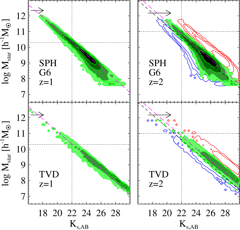
Figure 1: $K$-band magnitude versus stellar mass of simulated galaxies at $z=2$. The two dashed lines in the right column panels correspond to the relation found by Daddi et al. (2004b) from the K20 survey observational data (see text for details). In the right column panels, three sets of distributions are shown in blue, green, and red colors, corresponding to the extinction values $E(B-V)=0.0$, 0.4, and 1.0, respectively, with an arrow indicating the increasing extinction from 0.0 to 1.0. In the left column panels, only the case for $E(B-V)=0.4$ for $z=1$ is shown and the magenta dashed line is a similar relation to those in the right column panels with different normalization (see text for the exact value). The vertical dotted line indicates the magnitude limit of $K_{S}=22$, and the horizontal dotted line indicates the mass-scale of $M_{\star}=10^{10.3}{h^{-1}}{{\rm M}_{\odot}}$ for $z=1$ (left column) and $10^{11}{h^{-1}}{{\rm M}_{\odot}}$ for $z=2$ (right column).

In Figure 1, we plot the $K_{s}$ magnitude versus stellar mass for galaxies at $z=1$ and $2$, for SPH as well as TVD runs. In the right column panels, three sets of distributions are shown in blue, green, and red colors, respectively, corresponding to the extinction values $E(B-V)=0.0$, $0.4$, and $1.0$, with an arrow indicating the increasing extinction from 0.0 to 1.0. The two dashed lines in the right column panels for $z=2$ correspond to the relation found by Fontana et al. (2004) and Daddi et al. (2004b): $\log(M_{\star}/10^{11}{\rm M}_{\odot})=-0.4(K-K^{11})$, where $K_{AB}^{11}=21.37$ and 22.01 depends on the method used for the estimate. The good agreement between the simulation results and the observational relation is very encouraging. Slight deviations of the simulation results from the lines can be attributed to the scatter in the extinction value which is not taken into account in our theoretical calculations. In the left column panels, only the case for $E(B-V)=0.4$ is shown and the magenta dashed line is for $K_{AB}^{11}=20.7$.

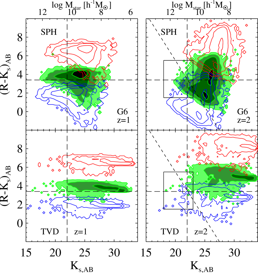
Figure 3: Color-magnitude diagram in the plane of $R-K_{s}$ color versus $K_{s}$-band magnitude for the SPH G6 run (upper row) and the TVD N864L22 run (bottom row) at $z=1$ (left column) and $z=2$ (right column). The top axes indicate the corresponding mass-scale obtained by the relation described in Section 5.1. The three different sets of distributions in each panel correspond to extinction values $E(B-V)=0.0$ (blue), 0.4 (green), and 1.0 (red). The magnitude limit of $K_{s}<22$ and the color-cut of $R-K_{s}>3.4$ (i.e., $(R-K)_{\rm vega}>5$) for the ERO selection is indicated by the vertical and horizontal long-dashed line, respectively. The square box shown in the right column panels encompasses the same region of space as Fig. 9 of Steidel et al. (2004), for comparison with a UV selected sample. The slanted short-dashed line in the right column panels indicates the constant magnitude limit of $R=25.5$.

Note that the scatter in the distribution of the simulated galaxies is much smaller compared with the same diagram as a function of $R$-band magnitude (Fig. 3 of Nagamine et al., 2005). This is because the $K$-band magnitude traces the stellar mass better than the $R$-band magnitude which probes the rest-frame UV wavelengths at $z=2-3$.

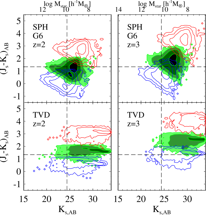
Figure 4: Color-magnitude diagram in the plane of $J_{s}-K_{s}$ color versus $K_{s}$-band magnitude for the SPH G6 run and the TVD run at $z=2$ and 3. The vertical dashed line indicates the magnitude limit of $K_{s}<24.4$ (i.e., $K_{\rm vega}\lesssim 22.5$), and the color-cut of $J_{s}-K_{s}>1.34$ (i.e., $(J_{s}-K_{s})_{\rm vega}>2.3$) is also shown as the horizontal dashed line. The four different colors represent different extinction values: $E(B-V)=0.0$ (blue), 0.4 (green), and 1.0 (red).

Also from this figure, we see that the magnitude limit of $K_{s}=22$ (i.e., $K_{s,{\rm vega}}=20$ mag) roughly corresponds to the stellar mass $M_{\star}\sim 10^{10.3}{h^{-1}}{{\rm M}_{\odot}}$ (at $z=1$) and $10^{11}{h^{-1}}{{\rm M}_{\odot}}$ (at $z=2$), as indicated by the vertical dotted line. As was shown in panel (a) of Fig. 4 in Nagamine et al. (2005), the corresponding number density at $z=2$ above the limit of $M_{\star}=10^{11}{h^{-1}}{{\rm M}_{\odot}}$ is $n(M_{\star}>10^{11}{h^{-1}}{{\rm M}_{\odot}})=3.5\times 10^{-4}\,h^{3}\,{\rm\,Mpc}^{-3}$ for the SPH G6 run, and $6.6\times 10^{-4}\,h^{3}\,{\rm\,Mpc}^{-3}$ for the TVD run. The number density at $z=2$ above the magnitude limit of $K_{s}=22$ is $n(K_{s}<22)=4.5\times 10^{-4}\,h^{3}\,{\rm\,Mpc}^{-3}$ for the SPH G6 run, and $5.6\times 10^{-4}\,h^{3}\,{\rm\,Mpc}^{-3}$ for the TVD run. The agreement between the two runs is reasonable when effects owing to the differences in boxsize, simulation methodology, and cosmic variance are taken into account.

We have repeated the same exercise at $z=3$. To summarize, we find that the following values of $K_{AB}^{11}$ describes the relation between the $K_{s}$ magnitude and the stellar mass of simulated galaxies: $K_{AB}^{11}=20.7$ (for z=1), 22.01 (for $z=2$, as given above by the K20 survey), and 23.0 (for z=3).

5.2 Color – magnitude diagrams

5.2.1 $I-K$ versus $I$ at $z=1$

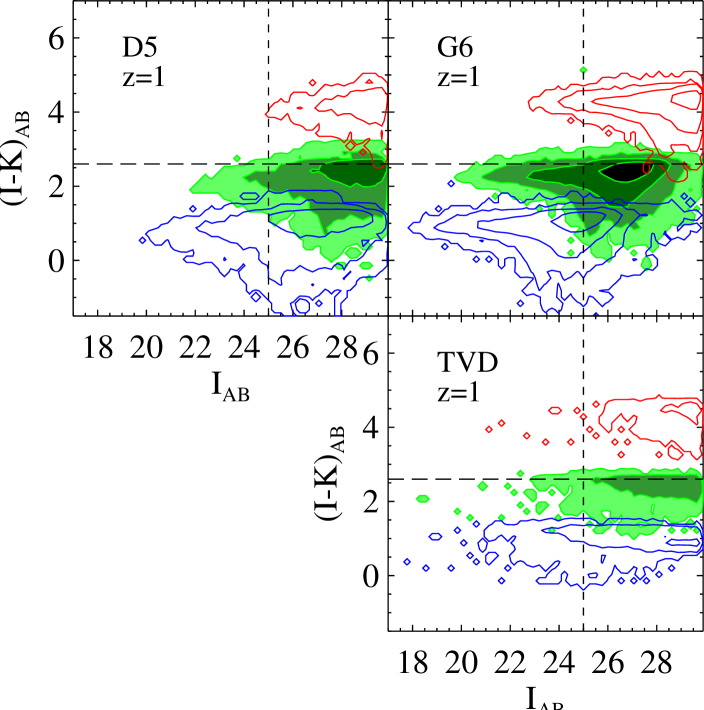
Figure 2: Color-magnitude diagram in the plane of $(I-K)_{AB}$ color versus $I_{AB}$-band magnitude for the SPH and TVD runs at $z=1$, corresponding to those of the GDDS (Abraham et al., 2004). The three different sets of distributions represent different extinction values: $E(B-V)=0.15$ (blue), 0.4 (green), and 1.0 (red). The magnitude limit of $I_{AB}=25$ of GDDS is indicated by the vertical dashed line. The color-cut $(I-K)_{AB}>2.6$ (i.e., $(I-K)_{\rm vega}>4$) for the ERO selection is also indicated as a long-dashed line.

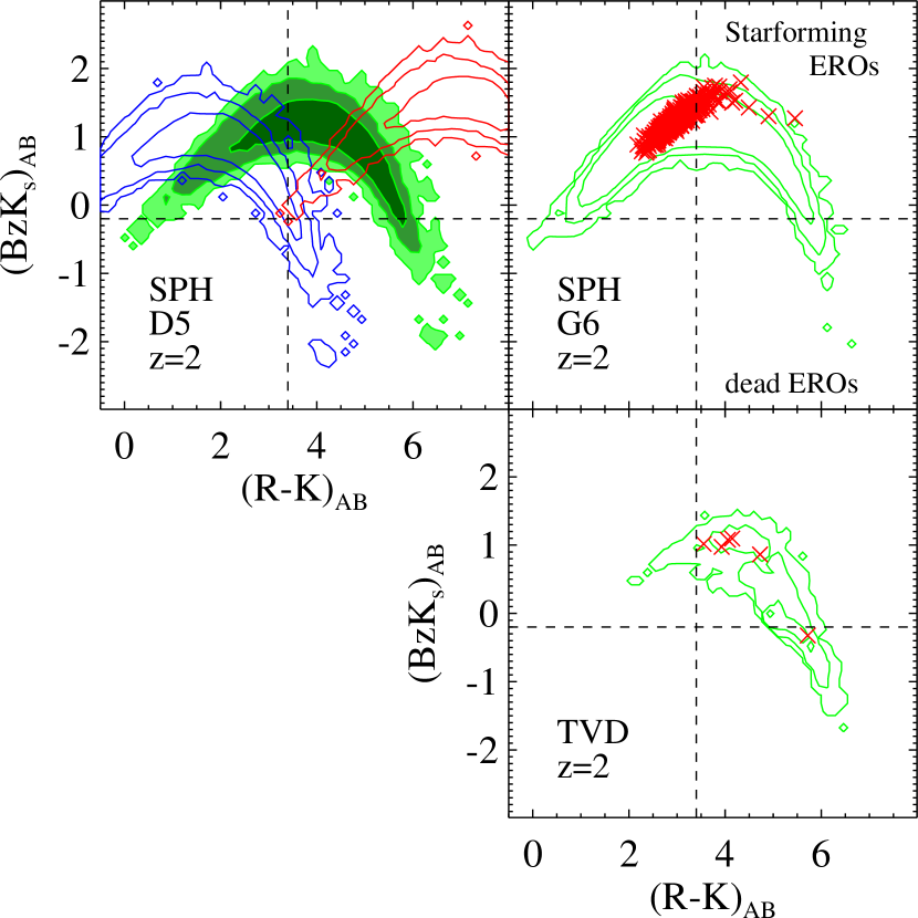
Figure 6: $BzK_{s}$ versus $R-K_{s}$ diagram of simulated galaxies at $z=2$, both for SPH and TVD runs. Similar to Figure 5, in the top left panel for the SPH D5 runs, three different sets of distributions are shown, corresponding to $E(B-V)=0.0$ (black), 0.4 (blue), and 1.0 (red). In the panels for the SPH G6 and TVD run, only the case of $E(B-V)=0.4$ is shown. The red crosses overplotted in the SPH G6 and the TVD panels are the galaxies that are brighter than $K_{s}=22$ (i.e., $K_{s,{\rm vega}}<20$).

Figure 2 shows the color-magnitude diagram of $I-K$ versus $K$-band magnitude at $z=1$, both for SPH and TVD simulations. This diagram corresponds to those presented by the GDDS group, e.g., Fig. 6 of Abraham et al. (2004) for galaxies at $z\sim 1$. The three different distributions represent different extinction values of $E(B-V)=0.0$ (blue), 0.4 (green), and 1.0 (red). The magnitude limit of $I_{AB}=25$ (i.e., $I_{\rm vega}=24.5$) of GDDS is indicated by the vertical dashed line. The color-cut $I-K>2.6$ (i.e., $(I-K)_{\rm vega}>4$) for the ERO selection is also indicated as a long-dashed line. Our simulations suggest extinction values of $E(B-V)\gtrsim 0.4$ for the EROs with $I-K>2.6$ at $z\sim 1$. Assuming $E(B-V)=0.4$ uniformly for the entire population, the corresponding number density of EROs at $z=1$ ($I<25$ and $I-K>2.6$) within the magnitude limit is $2.3\times 10^{-4}\,h^{3}\,{\rm\,Mpc}^{-3}$ for the SPH D5 run, $3.2\times 10^{-4}\,h^{3}\,{\rm\,Mpc}^{-3}$ for the SPH G6 run, and $2.5\times 10^{-3}\,h^{3}\,{\rm\,Mpc}^{-3}$ for the TVD run.

For comparison, the GDDS sample in McCarthy et al. (2004) with $(I-K)_{\rm vega}>4$ (16 objects) contributes $n=(3.4_{-1.2}^{+1.3})\times 10^{-4}\,h^{3}\,{\rm\,Mpc}^{-3}$ at $1.3<z<2$, in good agreement with our SPH results. The TVD run predicts a higher number density for the $I-K$ selected EROs at $z=1$ compared to the GDDS data.

5.2.2 $R-K_{s}$ versus $K_{s}$ at $z=1-3$

In Figure 3, we show the color-magnitude diagram of $R-K_{s}$ versus $K_{s}$-band magnitude at $z=1$ and $z=2$, both for the SPH G6 run and TVD runs. The top axes indicate the corresponding mass-scale obtained by the relation described in Section 5.1. In each panel, three different distributions are shown for extinctions $E(B-V)=0.0$ (blue), 0.4 (green), and 1.0 (red). The magnitude limit of $K_{s}=22$ and the color-cut of $R-K_{s}>3.4$ (i.e., $(R-K_{s})_{\rm vega}>5$) for the ERO selection is indicated by the long-dashed lines. Similarly to Fig. 2, our simulations suggest that extinction of $E(B-V)\gtrsim 0.4$ is needed to account for the EROs with $R-K_{s}>3.4$ at $z\sim 2$.

Assuming a uniform extinction of $E(B-V)=0.4$ for the entire population of simulated galaxies, the corresponding number density of EROs at $z=1-2$ that satisfy $K_{s}<22$ is summarized in Table 2. If we change the magnitude limit to $R<25.5$ instead (with $R-K_{s}>3.4$), we then obtain $5.0\times 10^{-5}\,h^{3}\,{\rm\,Mpc}^{-3}$ (SPH G6 run) and $3.8\times 10^{-4}\,h^{3}\,{\rm\,Mpc}^{-3}$ (TVD run) at $z=2$. At $z=3$ there are only a handful of galaxies that satisfy $R-K_{s}>3.4$ and $R<25.5$, and the numbers are clearly affected by the small statistics: $5.0\times 10^{-6}\,h^{3}\,{\rm\,Mpc}^{-3}$ for the SPH G6 run (5 objects in a $L_{\rm box}=100{h^{-1}}{\rm\,Mpc}$ box), and a null result for the TVD run.

Moustakas et al. (2004) estimated the space density of EROs using the GOODS data, finding $1.87\times 10^{-3}\,h^{3}\,{\rm\,Mpc}^{-3}$ for the EROs with $K_{s}<22$, $R-K_{s}>3.35$, and a median redshift of $z_{\rm med}=1.2$. The simulated number density of EROs at $z=1$ listed in Table 2 is slightly higher than their estimate, but they are reasonably close to each other considering the uncertainty in the distribution of the extinction parameter. Cimatti et al. (2002a) estimated the number density of EROs with $K_{\rm vega}<19.2$ and $(R-K_{s})_{\rm vega}>5$, and found $6.3\times 10^{-4}\,h^{3}\,{\rm\,Mpc}^{-3}$, whereas we find somewhat higher values of $1.4\times 10^{-3}\,h^{3}{\rm\,Mpc}^{-3}$ (SPH G6 run) and $2.0\times 10^{-3}\,h^{3}{\rm\,Mpc}^{-3}$ (TVD run) for the same magnitude limit and a uniform extinction of $E(B-V)=0.4$ at $z=1$. Väisänen & Johansson (2004) also estimated the ERO number density to be $\approx 5.8\times 10^{-5}\,h^{3}\,{\rm\,Mpc}^{-3}$ for the EROs with $K_{\rm vega}<17.5$, using the European Large Area ISO Survey (ELAIS) data. For the same magnitude limit and a uniform extinction of $E(B-V)=0.4$, we find $1.5\times 10^{-4}\,h^{3}\,{\rm\,Mpc}^{-3}$ (SPH G6 run) and $5.6\times 10^{-4}\,h^{3}\,{\rm\,Mpc}^{-3}$ (TVD run) at $z=1$. Saracco et al. (2005) obtained the comoving number density of $1.6\times 10^{-4}\,h^{3}\,{\rm\,Mpc}^{-3}$ for the EROs with $17.8<K<18.4$ and $(R-K)_{\rm vega}>5.3$ in the MUNICS data. In comparison, we find $3.3\times 10^{-4}\,h^{3}\,{\rm\,Mpc}^{-3}$ (SPH G6 run) and $1.9\times 10^{-4}\,h^{3}\,{\rm\,Mpc}^{-3}$ (TVD run) at $z=1$ for the same magnitude range and color-cut.

The number density of $R-K_{s}$ selected simulated galaxies (with $K_{s}<22$) is higher than that of $I-K$ selected (with $I<25$) galaxies. This is consistent with the finding of Väisänen & Johansson (2004) that the $R-K$ selected EROs have higher number counts than the $I-K$ selected EROs.

In the panels of the right column for $z=2$ in Figure 3, black square boxes that encompass the same region of space as Fig. 9 of Steidel et al. (2004) are shown. The dashed line indicates the constant magnitude limit of $R=25.5$, therefore, the observed data lie inside the box below this dashed line. We see that the simulated galaxies occupy a similar region in the color-magnitude plane as Steidel’s sample at $z=2$, suggesting some overlap between the near-IR selected sample and that of Steidel et al. (2004). The figure also suggests that the UV selected sample does not contain highly extincted galaxies with $E(B-V)\geq 0.75$.

5.2.3 $J_{s}-K_{s}$ versus $K_{s}$ at $z=2-3$

Figure 4 shows the color-magnitude diagram of $J_{s}-K_{s}$ color versus $K_{s}$-band magnitude, at redshifts $z=2$ and 3, both for SPH G6 run and TVD runs. This diagram has been used by the FIRES group (e.g. Franx et al., 2003; van Dokkum et al., 2004; Förster-Schreiber et al., 2004). The top axes indicate the corresponding mass-scale obtained by the relation described in Section 5.1. The three different distributions in each panel represent extinction values of $E(B-V)=0.0$ (blue), 0.4 (green), and 1.0 (red). The vertical short-dashed lines indicate the magnitude limit of $K_{s}<24.4$ (i.e., $K_{s,{\rm vega}}\lesssim 22.5$), and the color-cut of $J_{s}-K_{s}>1.34$ (i.e., $(J_{s}-K_{s})_{\rm vega}>2.3$) is shown as a horizontal long-dashed line.

Similar to Fig. 2, our simulations suggest extinction values of $E(B-V)\gtrsim 0.4$ for galaxies with $J_{s}-K_{s}>1.34$ at $z\sim 2$. Assuming $E(B-V)=0.4$ uniformly for the entire $z=2$ sample, the corresponding number densities for the above magnitude limit and the color-cut are $1.4\times 10^{-3}\,h^{3}\,{\rm\,Mpc}^{-3}$ for the SPH G6 run and $7.4\times 10^{-3}\,h^{3}\,{\rm\,Mpc}^{-3}$ for the TVD run. Similarly at $z=3$, $1.3\times 10^{-3}\,h^{3}\,{\rm\,Mpc}^{-3}$ for the SPH G6 run and $1.5\times 10^{-3}\,h^{3}\,{\rm\,Mpc}^{-3}$ for the TVD run.

Because the magnitude limit ($K_{s,AB}=24.4$) of FIRES is a few magnitudes deeper than that of the GDDS and the K20 survey, galaxies with stronger extinction ($E(B-V)\gtrsim 0.5$) can be sampled better, as seen in Fig. 4. This is in accordance with the fact that the amount of extinction estimated from the FIRES data is in the range $A_{V}=1-3$ mags, which corresponds to $E(B-V)=0.25-0.74$ for the Calzetti et al. (2000) extinction law. Comparison of Fig. 3 and Fig. 4 suggests that there would be a significant overlap between EROs (defined as $(R-K_{S})_{\rm vega}>5$) and DRGs (defined as $(J_{S}-K_{s})_{\rm vega}>2.3$), but the overlap may not be complete.

5.3 $BzK_{s}$ diagram at $z=2$

Recently, Daddi et al. (2004b) devised a new color-selection technique in order to separate star-forming galaxies and quiescent old galaxies for the $K_{s}$-band bright galaxies. They defined $BzK_{s}\equiv(z-K_{s})_{AB}-(B-z)_{AB}$, and demonstrated, using the K20 data, that the line of $BzK_{s}=-0.2$ in the color-color plane of $B-z$ versus $z-K_{s}$ (’$BzK_{s}$ diagram’) separates star-forming and quiescent old galaxies without star formation (indicated as ‘dead & red’) at $z>1.4$ quite nicely. The star-forming galaxies can hence be isolated in a $BzK_{s}$ diagram by $BzK>-0.2$, (upper left part of the plot) and the old galaxies by the criteria of $BzK_{s}<-0.2$ combined with $z-K_{s}>2.5$ (upper right corner of the plot). The $z-K_{s}>2.5$ criteria is similar to the commonly employed color-cut $R-K_{s}>5$ for selecting EROs. A convenient feature of this color separation technique is that the the extinction vector is almost parallel to the line of $BzK_{s}=-0.2$, therefore, the separation of the two populations is not strongly dependent on the amount of dust reddening.

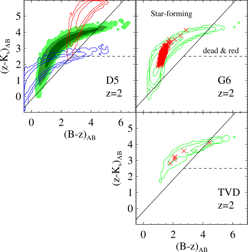
Figure 5: ‘BzK’ diagram at $z=2$ for the SPH and TVD runs. The lines $BzK_{s}=-0.2$ and $z-K_{s}=2.5$ are shown by the solid and the dashed lines, respectively. In the top left panel for the SPH D5 run, we show three different sets of distributions corresponding to $E(B-V)=0.0$ (blue), 0.4 (green), and 1.0 (red). The red crosses overplotted in the SPH G6 and the TVD panels are the galaxies that are brighter than $K_{s}=22$ (i.e., $K_{s,{\rm vega}}<20$).

Figure 5 shows the $BzK_{s}$ diagram of simulated galaxies at $z=2$, both for SPH and TVD runs. The lines $BzK_{s}=-0.2$ and $z-K_{s}=2.5$ are shown by the solid and the dashed lines, respectively. In the top left panel, for the SPH D5 run, we show three different distributions corresponding to $E(B-V)=0.0$ (blue), 0.4 (green), and 1.0 (red). In the panels for the SPH G6 and TVD runs, only the case for $E(B-V)=0.4$ is shown. The red crosses overplotted in the SPH G6 and the TVD panels are the galaxies that are brighter than $K_{s}=22$ (i.e., $K_{s,{\rm vega}}\lesssim 20$). In the SPH G6 run, all the red crosses are in the star-forming region, but in the TVD simulation there is one galaxy that satisfies $BzK_{s}<-0.2$ and $z-K_{s}>2.5$.

In the SPH G6 run, the corresponding number density of galaxies at $z=2$ with $K_{s}<22$ and $z-K_{s}>2.5$ is $2.2\times 10^{-4}h^{3}{\rm\,Mpc}^{-3}$. For the TVD run, we find $5.6\times 10^{-4}h^{3}{\rm\,Mpc}^{-3}$, but if we also require $BzK_{s}<-0.2$ we have $1.0\times 10^{-4}h^{3}{\rm\,Mpc}^{-3}$. These number densities are roughly consistent with the observed number density of $\sim 10^{-4}{\rm\,Mpc}^{-3}$ for galaxies with $K_{S,{\rm vega}}<20$ and $E(B-V)\sim 0.4$ by Daddi et al. (2004b). See Section 6 for further discussion on the comparison of our results with observations.

Figure 6 shows $BzK_{s}$ versus $R-K_{s}$ diagram of simulated galaxies at $z=2$ for both SPH and TVD runs. Similar to Figure 5, in the top left panel for the SPH D5 run, we show three distributions corresponding to extinction $E(B-V)=0.0$ (black), 0.4 (blue), and 1.0 (red). In the panels for the SPH G6 and TVD runs, only the case for $E(B-V)=0.4$ is shown. The red crosses overplotted in the SPH G6 and the TVD panels are the galaxies that are brighter than $K_{s}=22$ (i.e., $K_{s,{\rm vega}}<20$). This figure corresponds to Fig. 15 in Daddi et al. (2004b), in which they showed that about 50% of $BzK_{s}$ ($>-0.2$) selected galaxies at $z>1.4$ have ERO colors ($R-K_{s}>3.4$). In the SPH G6 run, 13% of galaxies at $z=2$ with $BzK_{s}>-0.2$ and $K_{s}<22$ satisfy the ERO color criteria, and the corresponding number density is $5.6\times 10^{-5}h^{3}{\rm\,Mpc}^{-3}$ for the star-forming EROs. In the TVD run, all galaxies brighter than $K_{s}=22$ satisfy the ERO color criteria for $E(B-V)=0.4$, and the corresponding number density is $5.6\times 10^{-4}h^{3}{\rm\,Mpc}^{-3}$.

5.4 Star formation histories of EROs

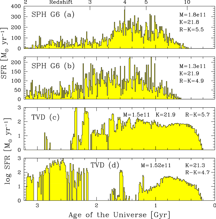
Figure 7: Star formation histories of the reddest EROs that satisfy $K_{s,AB}<22$ (i.e., $M_{\star}\gtrsim 1\times 10^{11}{h^{-1}}{{\rm M}_{\odot}}$) in our simulations. The top two panels show two galaxies from the G6 run z=2 output, and the bottom two panels show two galaxies from the TVD z=2 output (note the logarithmic scale of the ordinate). Panel (c) is the one in TVD run that satisfies the $BzK<-0.2$ criteria as well, being the only ‘dead & red’ massive ERO with $M_{\star}>1\times 10^{11}{h^{-1}}{{\rm M}_{\odot}}$. Note that this is a composite star formation history of all the progenitors that end up in the galaxy with properties indicated in the legend at $z=2$, therefore the early star formation may be attributed to several progenitors.

Figure 7 shows the star formation histories of the reddest EROs that satisfy $K_{s,AB}<22$ (i.e., $M_{\star}\gtrsim 1\times 10^{11}{h^{-1}}{{\rm M}_{\odot}}$) with a bin-size of 10 Myrs. The top two panels show two galaxies from G6 run z=2 output, and the bottom two panels show two galaxies from the TVD z=2 output (note the logarithmic scale of the ordinate). This is a composite star formation history of all the progenitors that end up in the galaxy with properties indicated in the legend at $z=2$, therefore the early star formation may be attributed to several progenitors.

Panel (c) is the one in the TVD run that satisfies the $BzK<-0.2$ criterion as well as the magnitude cut, formally being the only ‘dead, red, & old’ massive ERO with $M_{\star}>1\times 10^{11}{h^{-1}}{{\rm M}_{\odot}}$ according to the $BzK$ criteria. Indeed, this galaxy has built up most of its stellar mass by $z=3$, and star formation is almost absent between $z=3$ and $z=2$; i.e., passively evolving. On the other hand, the galaxy shown in panel (d) has little star formation in-between $z=5$ and $z=3$, but somewhat significant star formation in-between $z=3$ and $z=2$. This history allows it to pass the ERO criterion, but not the $BzK<-0.2$ criterion, and it does not qualify as a ‘dead, red, & old’ massive ERO.

The two EROs from the SPH G6 run shown in panels (a) and (b) experience a moderate peak of star formation in-between $z=5$ and $z=3$, but the star formation does not die away in-between $z=3$ and $z=2$, making it slightly too blue to satisfy the $BzK<-0.2$ criterion.

6 Discussion & Conclusions

We have used two different types of hydrodynamic cosmological simulations (Eulerian TVD and Lagrangian SPH) to study the properties of massive galaxies at $z=1-3$ in a $\Lambda$CDM universe. Our emphasis has been on the stellar mass and near-IR colors of galaxies, and on a comparison of our results with observations, including those of the GDDS, K20, FIRES, and GOODS surveys.

Our results suggest that hydrodynamic simulations based on the $\Lambda$CDM model do not exhibit the “mass-scale problem”; i.e. there is no obvious difficulty for the simulations to produce a sufficiently large number density of massive galaxies at high redshift, unlike some of the semi-analytic models. In particular, we find that the magnitude limit of $K_{s}=22$ (i.e., $K_{s,{\rm vega}}\simeq 20$ mag) of the K20 survey roughly corresponds to the stellar mass $M_{\star}\sim 10^{11}{h^{-1}}{{\rm M}_{\odot}}$ at $z=2$, and the number density above the magnitude limit is $\sim(3-6)\times 10^{-4}\,h^{3}\,{\rm\,Mpc}^{-3}$ at $z=2$. The simulated number density above the stellar mass limit of $M_{\star}>10^{11}{h^{-1}}{{\rm M}_{\odot}}$ agrees very well with these values. Our simulations can therefore account for the observed number density of massive galaxies found by the K20 survey.

The mean stellar mass of UV selected galaxies with $R<25.5$ at $z=2$ by Steidel et al. (2004) is $\left\langle\log M_{\star}\right\rangle\sim 10.3$, and their space density is $\sim 6\times 10^{-3}\,h^{3}\,{\rm\,Mpc}^{-3}$ (Erb et al., 2004). Therefore the mean stellar mass of the current UV selected sample is smaller by an order of magnitude than the K20 galaxies, while the number density is higher by an order of magnitude. Roughly $\lesssim 10$% of the UV selected sample has $K_{\rm vega}<20$, $M_{\star}>10^{11}{\rm M}_{\odot}$, $(J-K)_{\rm vega}>2.3$ (Erb et al., 2004), so currently the overlap between the K20 galaxies and the UV-selected galaxies by Steidel et al. (2004) seems to be at most 10% of the UV selected sample at $z\sim 2$. Of course, the UV selection will miss the reddest galaxies in the K20 sample. When the magnitude limit of the $K$-band selected sample is brought down to $K_{s}\sim 24$ (i.e., $K_{\rm vega}=22$, as already for the FIRES data), the $K$-band selected sample will contain galaxies with $M_{\star}\gtrsim 10^{10}\,{\rm M}_{\odot}$ at $z\sim 2$, and the space density of the two samples (UV selected and $K$-band selected) will be comparable at $\sim 6\times 10^{-3}\,h^{3}\,{\rm\,Mpc}^{-3}$. At that point, the overlap between the two samples may increase to a fraction higher than 10%. In Nagamine et al. (2005), we showed that the total number density of galaxies with $R<25.5$ in our simulations was about $2\times 10^{-2}\,h^{3}\,{\rm\,Mpc}^{-3}$ when a uniform extinction of $E(B-V)=0.15$ was assumed. This is twice the value of Erb et al.’s estimate, therefore we can obtain a consistent picture if the other half of the galaxies have higher extinction values $E(B-V)\gtrsim 0.4$ and can only be detected in the $K$-band survey.

The answer to the “redness problem” remains somewhat uncertain owing to the unknown dust content of the EROs and the number fraction of dusty star-forming galaxies within the observed ERO samples. We have studied the $I-K$, $R-K_{s}$, and $J_{s}-K_{S}$ colors of simulated galaxies by applying uniform extinction values to the entire samples. In all cases, our simulations suggest that the simulated EROs need to have extinction values greater than $E(B-V)=0.4$ in order to have colors as red as $(I-K)_{\rm vega}>4$, $(R-K_{s})_{\rm vega}>5$, or $(J_{s}-K_{s})_{\rm vega}>2.3$. This is consistent with the extinction values estimated for the EROs by observational means (e.g., Cimatti et al. 2002a; Daddi et al. 2004a; van Dokkum et al. 2004; Förster Schreiber et al. 2004).

The number density of EROs and DRGs (Distant Red Galaxies, see Section 2) in our simulations for a uniform extinction of $E(B-V)=0.4$ is summarized in Table 2. A robust comparison between theoretical models and observations is currently limited by our poor knowledge of the amount of dust in EROs and the number fraction of highly obscured starburst galaxies in the ERO samples. However, the numbers listed in Table 2 should serve as a benchmark for more stringent comparisons in the future. If the median extinction of EROs is close to $E(B-V)\sim 0.4$ as suggested by Daddi et al. (2004b), then the numbers summarized in Table 2 may not be so far from the actual values. This speculation is perhaps not so unreasonable as it may seem, because the recent morphological studies of EROs find that the fraction of early and late type is comparable at $30-40\%$ (e.g., Cimatti et al., 2003, 2004; Moustakas et al., 2004; Cassata et al., 2005). In this case, one may plausibly speculate that roughly half of the EROs have extinction smaller than $E(B-V)=0.4$, and the other half has $E(B-V)>0.4$.

As we described in Section 5.2.2, our simulations are able to account for the comoving number density of EROs of a few $\times 10^{-3}\,h^{3}\,{\rm\,Mpc}^{-3}$ at $z=1$ and a few $\times 10^{-4}\,h^{3}\,{\rm\,Mpc}^{-3}$ at $z=2$, provided we assume a uniform extinction of $E(B-V)=0.4$. These values are comparable to, or even slightly higher than the observational estimates (Cimatti et al., 2002a; Moustakas et al., 2004; Väisänen & Johansson, 2004; Daddi et al., 2004b). Taking this result at face value, our simulations do not appear to exhibit the “redness problem” either. However, as discussed in Section 5.3, if the observed number density of quiescent old EROs (that satisfy the criteria $K_{s}<22$, $BzK_{s}<-0.2$, and $z-K_{s}>2.5$) is really $\sim 1\times 10^{-4}\,h^{3}{\rm\,Mpc}^{-3}$, then the current SPH simulations underpredict the space density of such a population at $z=2$. The TVD simulation contained one such object, yielding the correct space density, but the statistical uncertainty of this result in a $L_{\rm box}=22{h^{-1}}{\rm\,Mpc}$ box is, of course, very large.

Since the space density of massive EROs is fairly low, large simulation boxsizes with $L_{\rm box}\gtrsim 100{h^{-1}}{\rm\,Mpc}$ are desired for future comparisons with observations. The controversial question is not just whether the hierarchical models can account for the space density of EROs, but it is the number density of quiescent, old, passively evolving EROs. It appears unlikely that our simulations have a problem in reproducing the space density of star-forming EROs. The $BzK_{s}$ diagram proposed by Daddi et al. (2004b) provides a useful test for this interesting population of old EROs which would otherwise be difficult to separate out clearly owing to dust confusion. Indeed, a recent study by Daddi et al. (2005) using the Hubble Ultra Deep Field data shows that the bulk of objects selected by $K_{s}<22$, $BzK<-0.2$, and $z-K>2.5$ are old and passive early types at redshifts $1.4<z<2.0$, with space density of $\sim 10^{-4}\,{\rm\,Mpc}^{-4}$. The “redness problem” is therefore perhaps better described as a “dead massive ERO problem”.

In this regard the connection between EROs and AGNs is intriguing. On the observational side, it is shown by Chandra and XMM-Newton that a sizable fraction ($\gtrsim 15$%) of the $2-10$ keV selected sources are associated with EROs (Rosati et al., 2002; Mainieri et al., 2002). The majority of the X-ray emitting EROs studied so far strongly suggests that the bulk of this population is composed of obscured AGNs, at least for the brightest X-ray fluxes (e.g., Alexander et al., 2002, 2003; Severgnini et al., 2005). On the theoretical side, Springel, DiMatteo, & Hernquist (2004) recently investigated the effect of AGN feedback during major mergers of gas-rich spiral galaxies using hydrodynamic simulations. Springel, DiMatteo, & Hernquist (2005) showed that mergers with black holes produce ellipticals that redden much faster owing to the suppression of further star formation by a strong outflow generated by the central black hole (see also Sazonov et al., 2005; Scannapieco & Oh, 2004), when feedback effects are normalized to reproduce the observed correlation between black hole mass and stellar velocity dispersion (Di Matteo, Springel, & Hernquist, 2005). Therefore, AGN feedback may play a critical role in producing red, old, and passively evolving massive EROs. This scenario can be tested with future cosmological simulations which self-consistently include black hole growth and AGN feedback processes.

Although the different simulation methods analyzed here broadly agree on the properties of high redshift galaxies, there are also interesting systematic differences between them. In general, the TVD run tends to predict a somewhat higher number density of EROs at all redshifts compared with the SPH simulations. This may owe to the fact that the star formation history in the TVD simulation is more sporadic than that of the SPH simulations, as we showed in Nagamine et al. (2005). Therefore at any given time, the stellar population of the simulated galaxies in the TVD run has more time to become redder between starbursts, without being so frequently affected by the blue light from the most recent star formation. This difference in the nature of the star formation history probably owes to a combination of differences in the details of the parameterization of the star formation physics, the strength of the feedback effects, the hydrodynamic methods, and the numerical resolution reached in the different simulations.

Finally, we comment on the differences between our hydrodynamic simulations and semi-analytic models of galaxy formation. As described in Section 1 and by Nagamine et al. (2004), our simulations have a star formation rate history that peaks at much higher redshift ($z\geq 5$) than that of most published semi-analytic models. We argue that this is one of the reasons why our hydrodynamic simulations are more successful in reproducing the properties of red massive galaxies at $z\sim 2$. Apparently, the star formation rate at high redshift ($z\geq 3$) is strongly suppressed by supernovae feedback in these semi-analytic models. While this helps them to match the faint-end of the galaxy luminosity function at $z=0$, they have problems in explaining EROs at high redshift. However, we note that a more recent revised version of the semi-analytic model by Baugh et al. (2005) enhances the burst-mode of star formation and obtains better agreement with the infra-red galaxy number counts and the redshift distribution of submillimeter galaxies at high redshift. Note that both TVD and SPH simulations (see Figure 7) automatically includes high amplitude bursts in response to infalling lumps of gas. Another revised semi-analytic model by Granato et al. (2004) incorporates the effects of AGN feedback, and now succeeds in producing red massive spheroidal galaxies at early times, also achieving better agreement with the observed infra-red to submillimeter galaxy counts (Silva et al., 2005). The results on the star formation rate history obtained by these recent semi-analytic models seem to be much closer to our hydrodynamic simulations and show more intense star formation at high redshifts. It would be interesting to see whether these revised semi-analytic models have the “dead massive ERO problem” by examining the $BzK$ diagrams of massive galaxies at $z\sim 2$.

Table 1: Simulations

Run	$L_{\rm box}$ [${h^{-1}}{\rm\,Mpc}$]	$N_{\rm mesh/ptcl}$	$m_{\rm DM}$ [${h^{-1}}{{\rm M}_{\odot}}$]	$m_{\rm gas}$ [${h^{-1}}{{\rm M}_{\odot}}$]	$\Delta\ell$ [${h^{-1}}{\rm\,kpc}$]
TVD: N864L22a	22.0	$864^{3}$	$8.9\times 10^{6}$	$2.2\times 10^{5}$	25.5
SPH: D5b	33.75	$324^{3}$	$8.2\times 10^{7}$	$1.3\times 10^{7}$	4.2
SPH: G6b	100.0	$486^{3}$	$6.3\times 10^{8}$	$9.7\times 10^{7}$	5.3

Note. — Parameters of the primary simulations on which this study is based. The quantities listed are as follows: $L_{\rm box}$ is the simulation box size, $N_{\rm mesh/ptcl}$ is the number of the hydrodynamic mesh points for TVD, or the number of gas particles for SPH, $m_{\rm DM}$ is the dark matter particle mass, $m_{\rm gas}$ is the mass of the baryonic fluid elements in a grid cell for TVD, or the masses of the gas particles in the SPH simulations. Note that TVD uses $432^{3}$ dark matter particles for N864 runs. $\Delta\ell$ is the size of the resolution element (cell size in TVD and gravitational softening length in SPH in comoving coordinates; for proper distances, divide by $1+z$). The upper indices on the run names correspond to the following sets of cosmological parameters: $(\Omega_{\rm M},\Omega_{\Lambda},\Omega_{b},h,n,\sigma_{8})=(0.29,0.71,0.047,0.7,1.0,0.85)$ for (a), and $(0.3,0.7,0.04,0.7,1.0,0.9)$ for (b).

Table 2: Number density of EROs and DRGs in the simulations

	$z=1$			$z=2$				$z=3$
	$(I-K)$	$(R-K_{s})$		$(R-K_{s})$	$(J_{s}-K_{s})$	$(z-K_{s})$		$(R-K_{s})$	$(J_{s}-K_{s})$
SPH	$(2-3)\times 10^{-4}$	$3.2\times 10^{-3}$		$5.6\times 10^{-5}$	$1.4\times 10^{-3}$	$2.2\times 10^{-4}$		$5.0\times 10^{-6}$	$1.3\times 10^{-3}$
TVD	$2.5\times 10^{-3}$	$4.2\times 10^{-3}$		$5.6\times 10^{-4}$	$7.4\times 10^{-3}$	$5.6\times 10^{-4}$		—	$1.5\times 10^{-3}$

Note. — Number density of EROs and DRGs in units of $h^{3}\,{\rm\,Mpc}^{-3}$ in our simulations satisfying the above color-selection and magnitude limit, assuming a uniform extinction of $E(B-V)=0.4$ for all galaxies. The density for the $R-K_{s}$ selection at $z=3$ is clearly affected by the limited boxsize, and is not very reliable. The number density for the $J_{s}-K_{s}$ selection is higher than other cases because of the deeper magnitude limit (corresponding to the FIRES data).

References

- Abraham et al. (2004) Abraham, R. G., Glazebrook, K., McCarthy, P. J., Crampton, D., Murowinski, R., Jørgensen, I., Roth, K., Hook, I. M., et al. 2004, AJ, 127, 2455
- Adelberger et al. (2004) Adelberger, K. L., Steidel, C. C., Shapley, A. E., Hunt, M. P., Erb, D. K., Reddy, N. A., & Pettini, M. 2004, ApJ, 607, 226
- Alexander et al. (2003) Alexander, D. M., Bauer, F. E., Brandt, W. N., et al. 2003, AJ, 126, 539
- Alexander et al. (2002) Alexander, D. M., Vignali, C., Bauer, F. E., et al. 2002, AJ, 123, 1149
- Barger et al. (2005) Barger, A. J., Cowie, L. L., Mushotzky, R. F., Yang, Y., Wang, W. H., Steffen, A. T., & Capak, P. 2005, AJ, 129, 578
- Barton et al. (2004) Barton, E. J., Davé, R., Smith, J.-D. T., Papovich, C., Hernquist, L., & Springel, V. 2004, ApJ, 605, L1
- Baugh et al. (2005) Baugh, C. M., Lacey, C. G., Frenk, C. S., Granato, G. L., Silva, L., Bressan A., Benson, A. J., & Cole, S. 2005, MNRAS, 356, 1191
- Brinchmann & Ellis (2000) Brinchmann, J. & Ellis, R. 2000, ApJ, 536, L77
- Bruzual & Charlot (2003) Bruzual, G. & Charlot, S. 2003, MNRAS, 344, 1000
- Calzetti et al. (2000) Calzetti, D., Armus, L., Bohlin, R. C., Kinney, A. L., Koornneef, J., & Storchi-Bergmann, T. 2000, ApJ, 533, 682
- Cassata et al. (2005) Cassata, P., Cimatti, A., Franceschini, A., Daddi, E., Pignatelli, E., Fasano, G., Rodighiero, G., Pozzetti, L., et al. 2005, MNRAS, 357, 903
- Cen (1992) Cen, R. 1992, ApJS, 78, 341
- Cen et al. (1994) Cen, R., Miralda-Escudé, J., Ostriker, J. P., & Rauch, M. 1994, ApJ, 437, L9
- Cen et al. (2004) Cen, R., Nagamine, K., & Ostriker, J. P. 2004, ApJ, submitted (astro-ph/0407143)
- Cen & Ostriker (1992) Cen, R. & Ostriker, J. P. 1992, ApJ, 399, L113
- Cen & Ostriker (1993) —. 1993, ApJ, 417, 404
- Cen & Ostriker (1999a) —. 1999a, ApJ, 514, 1
- Cen & Ostriker (1999b) —. 1999b, ApJ, 519, L109
- Cen & Ostriker (2000) —. 2000, ApJ, 538, 83
- Cen et al. (2003) Cen, R., Ostriker, J. P., Prochaska, J. X., & Wolfe, A. M. 2003, ApJ, 598, 741
- Chabrier (2003a) Chabrier, G. 2003a, ApJ, 586, L133
- Chabrier (2003b) —. 2003b, PASP, 115, 763
- Chapman et al. (2003) Chapman, S. C., Blain, A. W., Ivison, R. J., & Smail, I. R. 2003, Nature, 422, 695
- Cimatti et al. (2003) Cimatti, A., Daddi, E., Cassata, P., Pignatelli, E., Fasano, G., Vernet, J., Fomalont, E., Kellermann, K., et al. 2003, A&A, 412, L1
- Cimatti et al. (2002a) Cimatti, A., Daddi, E., Mignoli, M., Pozzetti, L., Renzini, A., Zamorani, G., Broadhurst, T., Fontana, A., et al. 2002a, A&A, 381, L68
- Cimatti et al. (2004) Cimatti, A., Daddi, E., Renzini, A., Cassata, P., Vanzella, E., Pozzetti, L., Cristiani, S., Fontana, A., et al. 2004, Nature, 430, 184
- Cimatti et al. (2002b) Cimatti, A., Mignoli, M., Daddi, E., Pozzetti, L., Fontana, A., Saracco, P., Poli, F., Renzini, A., et al. 2002b, A&A, 392, 395
- Cimatti et al. (2002c) Cimatti, A., Pozzetti, L., Mignoli, M., Daddi, E., Menci, N., Poli, F., Fontana, A., Renzini, A., et al. 2002c, A&A, 391, L1
- Cohen (2002) Cohen, J. G. 2002, ApJ, 567, 672
- Cole et al. (2000) Cole, S., Lacey, C. G., Baugh, C. M., & Frenk, C. S. 2000, MNRAS, 319, 168
- Cole et al. (2001) Cole, S., Norberg, P., Baugh, C. M., Frenk, C. S., Bland-Hawthorn, J., Bridges, T., Cannon, R., Colless, M., Collins, C., et al. 2001, MNRAS, 326, 255
- Connolly et al. (1997) Connolly, A. J., Szalay, A. S., Dickinson, M. E., SubbaRao, M. U., & Brunner, R. J. 1997, ApJ, 486, L11
- Cowie et al. (1999) Cowie, L. L., Songaila, A., & Barger, A. J. 1999, AJ, 118, 603
- Daddi et al. (2004a) Daddi, E., Cimatti, A., Renzini, A., Vernet, J., Conselice, C., Pozzetti, L., Mignoli, M., Tozzi, P., et al. 2004a, ApJ, 600, L127
- Daddi et al. (2004b) —. 2004b, ApJ, 617, 746
- Daddi et al. (2005) Daddi, E., Renzini, A., Pirzkal, N., Cimatti, A., Malhotra, S., Stiavelli, M., Xu, C., Pasquali, A., et al. 2005, ApJ, 626, 680
- Davé et al. (1999) Davé, R., Hernquist, L., Katz, N., & Weinberg, D. H. 1999, ApJ, 511, 521
- Di Matteo et al. (2005) Di Matteo, T., Springel, V., & Hernquist, L. 2005, Nature, 433, 604
- Dickinson et al. (2003) Dickinson, M., Papovich, C., Ferguson, H., & Budavári, T. 2003, ApJ, 587, 25
- Drory et al. (2001) Drory, N., Feulner, G., Bender, R., et al. 2001, MNRAS, 325, 550
- Elston et al. (1988) Elston, R., Rieke, G. H., & Rieke, M. 1988, ApJ, 331, L77
- Erb et al. (2004) Erb, D. et al. 2004, in Starbursts - from 30 Doradus to Lyman break galaxies, ed. de Grijs R. & Gonzalez Delgado R.M. (Astrophysics & Space Science Library, Kluwer: Dordrecht)
- Fan et al. (2001) Fan, X., Strauss, M. A., Schneider, D. P., Gunn, J. E., Lupton, R. H., Becker, R. H., Davis, M., Newman, J. A., et al. 2001, AJ, 121, 54
- Fontana et al. (2003) Fontana, A., Donnarumma, I., Vanzella, E., Giallongo, E., Menci, N., Nonino, M., Saracco, P., Cristiani, S., et al. 2003, ApJ, 594, L9
- Fontana et al. (2004) Fontana, A., Pozzetti, L., Donnarumma, I., Renzini, A., Cimatti, A., Zamorani, G., Menci, N., Daddi, E., et al. 2004, A&A, 424, 23
- Förster-Schreiber et al. (2004) Förster-Schreiber, N. M., van Dokkum, P. G., Franx, M., Labbe, I., Rudnick, G., Daddi, E., Illingworth, G. D., Kriek, M., et al. 2004, ApJ, 616, 40
- Franx et al. (2003) Franx, M., Labbe, I., Rudnick, G., van Dokkum, P. G., Daddi, E., Förster, S., Natascha, M., Moorwood, A., et al. 2003, ApJ, 587, L79
- Furlanetto et al. (2004e) Furlanetto, S. R., Hernquist, L., & Zaldarriaga, M. 2004e, MNRAS, 354, 695
- Furlanetto et al. (2003) Furlanetto, S. R., Schaye, J., Springel, V., & Hernquist, L. 2003, ApJ, 599, L1
- Furlanetto et al. (2004d) —. 2004d, ApJ, 606, 221
- Furlanetto et al. (2004a) Furlanetto, S. R., Sokasian, A., & Hernquist, L. 2004a, MNRAS, 347, 187
- Furlanetto et al. (2004b) Furlanetto, S. R., Zaldarriaga, M., & Hernquist, L. 2004b, ApJ, 613, 16
- Furlanetto et al. (2004c) —. 2004c, ApJ, 613, 1
- Glazebrook et al. (2004) Glazebrook, K., Abraham, R., McCarthy, P., Savaglio, S., Chen, H.-W., Crampton, D., Murowinski, R., Jorgensen, I., et al. 2004, Nature, 430, 181
- Granato et al. (2000) Granato, G. L., Lacey, C. G., Silva, L., Bressan, A., Baugh, C. M., Cole, S., & Frenk, C. S. 2000, ApJ, 542, 710
- Granato et al. (2004) Granato, G. L., De Zotti, G., Silva, L., Bressan, & Danese, L. 2004, ApJ, 600, 580
- Hayes (1985) Hayes, D. S. 1985, in Calibration of Fundamental Stellar Quantities, IAU Symposium 111, ed. D. S. Hayes et al. (Dordrecht, Reidel), 225
- Hernquist (1993) Hernquist, L. 1993, ApJ, 404, 717
- Hernquist & Springel (2003) Hernquist, L. & Springel, V. 2003, MNRAS, 341, 1253
- Hu et al. (1999) Hu, E. M., McMahon, R. G., & Cowie, L. L. 1999, ApJ, 522, L9
- Hu & Ridgway (1994) Hu, E. M. & Ridgway, S. E. 1994, AJ, 107, 1303
- Iwata et al. (2003) Iwata, I., Ohta, K., Tamura, N., Ando, M., Wada, S., Watanabe, C., Akiyama, M., & Aoki, K. 2003, PASJ, 55, 415
- Katz et al. (1996) Katz, N., Weinberg, D. H., & Hernquist, L. 1996, ApJS, 105, 19
- Kauffmann et al. (1999) Kauffmann, G., Colberg, J. M., Diaferio, A., & White, S. D. M. 1999, MNRAS, 303, 188
- Kodaira et al. (2003) Kodaira, K., Taniguchi, Y., Kashikawa, N., Kaifu, N., Ando, H., Karoji, H., Ajiki, M., Akiyama, M., et al. 2003, PASJ, 55, L17
- Kroupa (2001) Kroupa, P. 2001, MNRAS, 322, 231
- Kurucz (1992) Kurucz, R. L. 1992, in The Stellar Populations of Galaxies, IAU Symposium, ed. B. Barbuy & A. Renzini, 225
- Lilly et al. (1996) Lilly, S. J., Fèvre, O. L., Hammer, F., & Crampton, D. 1996, ApJ, 460, L1
- Madau (1995) Madau, P. 1995, ApJ, 441, 18
- Mainieri et al. (2002) Mainieri, V., Bergeron, J., Hasinger, G., et al. 2002, A&A, 393, 425
- McCarthy (2004) McCarthy, P. J. 2004, ARA&A, 42, 477
- McCarthy et al. (2004) McCarthy, P. J., Le Borgne, D., Crampton, D., Chen, H.-W., Abraham, R. G., Glazebrook, K., Savaglio, S., Carlberg, R. G., et al. 2004, ApJ, 614, L9
- McCarthy et al. (1992) McCarthy, P. J., Persson, S. E., & West, S. C. 1992, ApJ, 386, 52
- Menci et al. (2002) Menci, N., Cavaliere, A., Fontana, A., Giallongo, E., & Poli, F. 2002, ApJ, 575, 18
- Moustakas et al. (2004) Moustakas, L. A., Casertano, S., Conselice, C., Dickinson, M. E., Eisenhardt, P., Ferguson, H., Giavalisco, M., et al. 2004, ApJ, 600, L131
- Nagamine (2002) Nagamine, K. 2002, ApJ, 564, 73
- Nagamine et al. (2004) Nagamine, K., Cen, R., Hernquist, L., Ostriker, J. P., & Springel, V. 2004, ApJ, 610, 45
- Nagamine et al. (2005) —. 2005, ApJ, 618, 23
- Nagamine et al. (2001a) Nagamine, K., Fukugita, M., Cen, R., & Ostriker, J. P. 2001a, ApJ, 558, 497
- Nagamine et al. (2001b) —. 2001b, MNRAS, 327, L10
- Nagamine et al. (2004a) Nagamine, K., Springel, V., & Hernquist, L. 2004a, MNRAS, 348, 421
- Nagamine et al. (2004b) —. 2004b, MNRAS, 348, 435
- Nagamine et al. (2004c) Nagamine, K., Springel, V., Hernquist, L., & Machacek, M. 2004c, MNRAS, 350, 385
- Night et al. (2005) Night, C., Nagamine, K., Springel, V., & Hernquist, L. 2005, MNRAS, submitted (astro-ph/0503631)
- Ouchi et al. (2003) Ouchi, M., Shimasaku, K., Furusawa, H., Miyazaki, M., Doi, M., Hamabe, M., Hayashino, T., Kimura, M., et al. 2003, ApJ, 582, 60
- Ouchi et al. (2004) —. 2004, ApJ, 611, 660
- Pascarelle et al. (1998) Pascarelle, S. M., Lanzetta, K. M., & Fernandez-Soto, A. 1998, ApJ, 508, L1
- Poli et al. (2003) Poli, F., Giallongo, E., Fontana, A., Menci, N., Zamorani, G., Nonino, M., Saracco, P., Vanzella, E., et al. 2003, ApJ, 593, L1
- Rhoads & Malhotra (2001) Rhoads, J. E. & Malhotra, S. 2001, ApJ, 563, L5
- Robertson et al. (2004) Robertson, B. E., Yoshida, N., Springel, V., & Hernquist, L. 2004, ApJ, 606, 32
- Rosati et al. (2002) Rosati, P., Tozzi, P., Giacconi, R., et al. 2002, ApJ, 566, 667
- Rudnick et al. (2003) Rudnick, G., Rix, H.-W., Franx, M., Labbe, I., Blanton, M., Daddi, E., Förster, S., Natascha, M., et al. 2003, ApJ, 599, 847
- Ryu et al. (1993) Ryu, D., Ostriker, J. P., Kang, H., & Cen, R. 1993, ApJ, 414, 1
- Saracco et al. (2003) Saracco, P., Longhetti, M., Severgnini, P., Ceca, R. D., Mannucci, F., Bender, R., Drory, N., Feulner, G., et al. 2003, A&A, 398, 127
- Saracco et al. (2004) Saracco, P., Longhetti, M., Giallongo, E., Arnouts, S., Cristiani, S., D’Odorico, S., Fontana, A., Nonino, M., & Vanzella, E. 2004, A&A, 420, 125
- Saracco et al. (2005) Saracco, P., Longhetti, M., Severgnini, P., Ceca, R. D., Braito, V., Mannucci, F., Bender, R., Drory, N., et al. 2005, MNRAS, 357, L40
- Sawicki et al. (1997) Sawicki, M. J., Lin, H., & Yee, H. K. C. 1997, AJ, 113, 1
- Sazonov et al. (2005) Sazonov, S. Y., Ostriker, J. P., Ciotti, L., & Sunyaev, R. A. 2005, MNRAS, 358, 168
- Scannapieco & Oh (2004) Scannapieco, E. & Oh, S. P. 2004, ApJ, 608, 62
- Schmidt (1968) Schmidt, M. 1968, ApJ, 151, 393
- Schmidt et al. (1995) Schmidt, M., Schneider, D. P., & Gunn, J. E. 1995, AJ, 110, 68
- Severgnini et al. (2005) Severgnini, P., Ceca, R. D., Braito, V., Longhetti, P. S. M., Bender, R., Drory, N., Feulner, G., et al. 2005, A&A, 431, 87
- Silva et al. (2005) Silva, L., De Zotti, G. Granato, G. L., Maiolino, R., & Danese, L. 2005, MNRAS, 357, 1295
- Smail et al. (1997) Smail, I., Ivison, R. J., & Blain, A. W. 1997, ApJ, 490, L5
- Smail et al. (2002) Smail, I., Owen, F. N., Morrison, G. E., Keel, W. C., Ivison, R. J., & Ledlow, M. J. 2002, ApJ, 581, 844
- Somerville et al. (2004) Somerville, R. S., Moustakas, L. A., Mobasher, B., Gardner, J. P., Cimatti, A., Conselice, C., Daddi, E., Dahlen, T., et al. 2004, ApJ, 600, L135
- Somerville et al. (2001) Somerville, R. S., Primack, J. R., & Faber, S. M. 2001, MNRAS, 320, 504
- Spergel et al. (2003) Spergel, D., Verde, L., Peiris, H. V., Komatsu, E., Nolta, M. R., Bennett, C. L., Halpern, M., Hinshaw, G., et al. 2003, ApJS, 148, 175
- Springel et al. (2005) Springel, V., DiMatteo, T., & Hernquist, L. 2005, ApJ, 620, L79
- Springel et al. (2004) —. 2004, MNRAS, submitted (astro-ph/0411108)
- Springel & Hernquist (2002) Springel, V. & Hernquist, L. 2002, MNRAS, 333, 649
- Springel & Hernquist (2003a) —. 2003a, MNRAS, 339, 289
- Springel & Hernquist (2003b) —. 2003b, MNRAS, 339, 312
- Springel et al. (2001) Springel, V., Yoshida, N., & White, S. D. M. 2001, New Astronomy, 6, 79
- Steidel et al. (1999) Steidel, C. C., Adelberger, K. L., Giavalisco, M., Dickinson, M., & Pettini, M. 1999, ApJ, 519, 1
- Steidel & Hamilton (1993) Steidel, C. C. & Hamilton, D. 1993, AJ, 105, 2017
- Steidel et al. (2004) Steidel, C. C., Shapley, A. E., Pettini, M., Adelberger, K. L., Erb, D. K., Reddy, N. A., & Hunt, M. P. 2004, ApJ, 604, 534
- Taniguchi et al. (2003) Taniguchi, Y., Ajiki, M., Murayama, T., Nagao, T., Veilleux, S., Sanders, D. B., Komiyama, Y., Shioya, Y., et al. 2003, ApJ, 585, L97
- Treyer et al. (1998) Treyer, M. A., Ellis, R. S., Millard, B., Donas, J., & Bridges, T. J. 1998, MNRAS, 300, 303
- Väisänen & Johansson (2004) Väisänen, P. & Johansson, P. H. 2004, A&A, 421, 821
- van Dokkum et al. (2004) van Dokkum, P., Franx, M., Schreiber, N. F., Illingworth, G., Daddi, E., Knudsen, K. K., Labbe, I., Moorwood, A., et al. 2004, ApJ, 611, 703
- Zaldarriaga et al. (2004) Zaldarriaga, M., Furlanetto, S. R., & Hernquist, L. 2004, ApJ, 608, 622