A numerical comparison of theories of violent relaxation

Abstract

Using $N$-body simulations with a large set of massless test particles we compare the predictions of two theories of violent relaxation, the well known Lynden-Bell theory and the more recent theory by Nakamura. We derive “weakened” versions of both theories in which we use the whole equilibrium coarse-grained distribution function $\bar{f}_{i}$ as a constraint instead of the total energy constraint. We use these weakened theories to construct expressions for the conditional probability $K_{i}(\tau)$ that a test particle initially at the phase-space coordinate $\tau$ would end-up in the $i$’th macro-cell at equilibrium. We show that the logarithm of the ratio $R_{ij}(\tau)\equiv K_{i}(\tau)/K_{j}(\tau)$ is directly proportional to the initial phase-space density $f_{0}(\tau)$ for the Lynden-Bell theory and inversely proportional to $f_{0}(\tau)$ for the Nakamura theory. We then measure $R_{ij}(\tau)$ using a set of $N$-body simulations of a system undergoing a gravitational collapse to check the validity of the two theories of violent relaxation. We find that both theories are at odds with the numerical results, both qualitatively and quantitatively.

1 Introduction

A statistical theory that successfully describes the process of a collisionless gravitational collapse has been a longstanding open problem. The ultimate goal of such a theory is to predict the (semi-) equilibrium state of a gravitational system that is described by the Vlasov equation, given its initial phase-space density $f_{0}(\mathbf{r},\mathbf{v})$. The implications of such a theory to cosmology and astrophysics are immense. For example, such a theory may be able to explain the origin of cusps found in simulations of CDM haloes, the universality of their shape, and possibly connect them to the initial cold phase-space density distribution.

The first attempt to construct such a theory was made by Lynden-Bell in his pioneering work from 1967 (Lynden-Bell, 1967, hereafter the LB67 theory) which actually coined the phrase “violent relaxation” to describe the relaxation of such systems. However, already in that paper Lynden-Bell predicted that his theory will not be applicable to large parts of the system due to the “incompleteness of violent relaxation”. The fluctuations of the gravitational potential, which drive the system towards an equilibrium state fade out too soon for the system to explore the full configuration space. Therefore the final equilibrium state picked by the system is not necessarily the one that maximises the entropy. The discrepancy becomes larger as we go from the centre of the system to its outer parts where the gravitational fluctuations are much smaller. Accordingly, Lynden-Bell assumed that the complete relaxation is limited to a sphere of radius $R_{1}$ around the system’s centre of mass.

Soon after this paper, many $N$-body simulations were run to check its validity. Most of these simulations were of one-dimensional models of either plane sheets or of spherical shells (Cohen & Lecar, 1968; Hénon, 1968; Cuperman at el., 1969; Goldstein et al., 1969; Lecar & Cohen, 1971; Tanekusa, 1987). In most cases the LB67 theory was only partially correct at best. A common outcome of the “water-bucket” initial conditions (in which there is only one level of phase-space density surrounded by a vacuum) was the “core-halo” structure in which the halo took most of the energy of the system, leaving the core (which contained most of the mass) degenerate. Compared with predictions, the phase-space density was too high at very low energies, too low at intermediate energies, and oscillated at high energies. One can find a good fit for the core using the degenerate solution of the LB67 theory, and a reasonable fit for the halo using the non-degenerate solution - but then it is difficult to find a clean way to decide which particles should be described by which one of the two solutions. Consequently, the theory loses much of its predictive power. This ambiguity was attributed to the incompleteness of the relaxation: the inner parts where the relaxation was effective could be described by a LB67 solution, unlike the outer parts which were only partially relaxed.

The disagreement between the predictions of the LB67 theory and experiments, in addition to some disturbing conceptual issues it possesses (such as its infinite mass prediction in 3D and phase-space densities segregation - see Sec. 2.3 for further details), have led people to consider alternatives to it, e.g., Shu (1978); Stiavelli & Bertin (1987); Spergel & Hernquist (1992); Kull et al. (1997); Nakamura (2000); Trenti & Bertin (2005). In all these theories the equilibrium state is assumed to be the most probable state of the system, which is found by maximising the entropy under the appropriate constraints. The difference between these theories is mainly due to the definition of entropy they use and the constraints under which it is maximised.

For the purpose of this paper we roughly divide these theories into two groups: in the first group we have theories which are based on a more fundamental approach to the problem, thereby incorporating (almost) all of the dynamical constraints when maximising the entropy. In this group we essentially have two theories: the theory of Lynden-Bell (1967) and the theories of Kull et al. (1997) and Nakamura (2000), which as we shall see, are basically the same theory. In the second group we have theories that use more heuristic, ad-hoc like, constraints and entropy definitions, such as Stiavelli & Bertin (1987); Spergel & Hernquist (1992); Trenti & Bertin (2005), or Hansen et al. (2005) who use non-extensive statistical mechanics, and to some extent Shu (1978). Non of these theories, for example, take into account the conservation of the phase-space volume by the dynamics, as required by Liouville’s theorem. As a rule of thumb, the predictions of the second group are in a better agreement with simulations and observations than the first group. However, this is achieved at the expense of increasing the number of assumptions and free parameters in the theory. In this paper we are interested in examining how well the fundamental assumptions of statistical mechanics apply in violent relaxation, we shall therefore concentrate on the first group of theories: the LB67 theory and the theory of Nakamura (2000) (hereafter NK00).

The purpose of this paper is three-fold: firstly, we wish to compare the predictions of the LB67 and NK00 theories with numerical experiments done in 3D. To our knowledge this has not yet been done directly, in particular when it comes to the NK00 theory. While the 1D case shares many common characteristics with the 3D case, it is known that dimensionality may play an important role in systems undergoing violent relaxation. For example, the 3D system has more degrees of freedom, and may therefore experience a more efficient mixing. Indirect support for the NK00 theory in $3D$ is found in Merrall & Henriksen (2003). Here the authors show that the velocity distribution function of isolated systems after violent relaxation is well fitted by a single Gaussian, as is predicted by the NK00 theory for the non-degenerate case. Nevertheless, we would like to perform a more direct test of the predictions of this theory.

Secondly, acknowledging the fact that these theories are largely incorrect, we would still like to see if certain aspects of them are true. In other words, we would like to see if the approach of maximising the entropy under the proper constraints is at all useful in the weakest possible sense for a dissipationless self-gravitating system. Thirdly, as we shall see in Sec. 2, the NK00 theory and the LB67 theory have a very similar structure, incorporating the same set of constraints, while using fundamentally different entropy definitions. We would therefore like to know which definition describes violent relaxation better. We feel that somehow the question of how entropy should be defined is more fundamental than the full statistical theory around it. For example, a local definition of entropy can be used in a dynamical theory that describes the approach to equilibrium [e.g. Chavanis (1998)].

The structure of this paper is as follows: in Sec. 2 we review the LB67 and NK00 theories and derive them using the information-theory approach. We introduce the conditional and joint probabilities that describe the path of a test particle and relate them to the different definitions of entropy between the two theories. We then list some of the problems and questions with these theories and re-derive “weakened” versions of the theories. We show how the predictions of these theories can be tested in a numerical experiment that to a large extent avoids many of the pitfalls we would have encountered had we tried to test the LB67 and NK00 theories in their original form. In Sec. 3 we describe how the conditional probabilities can be measured in an $N$-body simulation using a large number of test particles. Then in Sec. 4 we describe the numerical simulations that we have performed to measure these probabilities and in Sec. 5 we present the results of the simulations. Our conclusions are presented in Sec. 6.

2 Theoretical background - two theories for violent relaxation

In this section we will focus on the LB67 theory and a more recent alternative to it - the NK00 theory. The aim of these theories is to predict the final equilibrium state of a collisionless gravitating system, given its initial state. The state of the system is completely determined by its phase-space density function (DF) $f(\mathbf{r},\mathbf{v},t)$, which is governed by the Vlasov equation

$$\partial_{t}f+\mathbf{v}\cdot\partial_{\mathbf{r}}f-\nabla\Phi\cdot\partial_{\mathbf{v}}f=0\ .$$ (1)

Here $\Phi(\mathbf{r},t)$ is the gravitational potential, calculated self-consistently from $\rho(\mathbf{r},t)=\int\!\!f(\mathbf{r},\mathbf{v},t)d^{3}\mathbf{v}$ via Poisson’s equation.

2.1 Derivation of the NK00 theory

The NK00 theory was originally derived in the framework of information theory. Here we shall repeat its derivation for comparison with the LB67 theory. We first formulate the violent relaxation process as an experiment with a well defined set of possible results $\omega_{i}$ and a set of corresponding probabilities $p_{i}$. The most probable result is then the one that maximises the Shannon entropy $S=\sum_{i}p_{i}\log p_{i}$ under some prescribed constraints on $p_{i}$ (Jaynes, 1957a, b).

Let $f_{0}(\tau)$ be the initial phase-space density of the system, with $\tau\equiv(\mathbf{r},\mathbf{v})$ being a phase-space coordinate. We toss a test particle into the initial phase-space according to the probability distribution $p_{0}(\tau)$ which is defined by

$$p_{0}(\tau)=\frac{1}{M}f_{0}(\tau)\ ,$$ (2)

and let it move under gravity just like any phase-space element. We define $p(\tau,t)$ to be the probability distribution of finding the test particle at time $t>0$. The conservation of phase-space volume guarantees that $p(\tau,t)=f(\tau,t)/M$ for all $t>0$.

Next, we divide phase-space into macro-cells $i=1,2,3,\ldots$ of volume $\tilde{\omega}$, and define the coarse-grained probability $\bar{p}_{i}$ as the probability of finding the test particle in the $i$’th macro-cell when the system reaches an equilibrium. From the above discussion it is clear that $\bar{p}_{i}$ is equal to $\bar{f}_{i}/M$ with $\bar{f}_{i}$ being the coarse-grained DF in the macro-cell $i$ at equilibrium.

A possible result of our experiment is the pair $(\tau,i)$ which specifies the initial location of the test particle and the number of the cell where it is finally found. With each such pair we associate the joint probability-distribution $p_{i}(\tau)$. $p_{i}(\tau)d^{6}\tau$ is the probability that the particle was initially in a small patch of volume $d^{6}\tau$ around $\tau$, and ended up in the $i$’th macro-cell. The Shannon entropy of our experiment is then

$$S_{NK}=-\sum_{i}\int\!\!d^{6}\tau\,p_{i}(\tau)\log p_{i}(\tau)\ .$$ (3)

Maximising $S_{NK}$ gives us the most probable $p_{i}(\tau)$, from which we can get

$$\bar{f}_{i}=M\int\!p_{i}(\tau)d^{6}\tau\ .$$ (4)

Before maximising $S_{NK}$, however, we must write down the constraints on the probabilities $p_{i}(\tau)$. The first constraint stems from the initial conditions and from the fact that $p_{i}(\tau)$ is a joint probability distribution:

$$\sum_{i}p_{i}(\tau)=p_{0}(\tau)=\frac{1}{M}f_{0}(\tau)\ .$$ (5)

The second constraint comes from the conservation of phase-space volume under the collisionless dynamics: the overall initial phase-space volume of all phase-space elements that ended up in cell $i$ will be exactly $\tilde{\omega}$:

$$M\int\!\!d^{6}\tau\frac{p_{i}(\tau)}{f_{0}(\tau)}=\tilde{\omega}\ .$$ (6)

This constraint guarantees that the NK00 theory does not violate Liouville’s theorem. Finally, from the conservation of energy, the total energy in $\bar{f}_{i}$ must be equal to the initial energy of the system $E$

$$E=\sum_{i}\tilde{\omega}\bar{f}_{i}\left[\frac{v^{2}_{i}}{2}+\frac{G}{2}\sum_{j}\frac{\tilde{\omega}\bar{f}_{j}}{|\mathbf{r}_{i}-\mathbf{r}_{j}|}\right]\ ,$$ (7)

with $(\mathbf{r}_{i},\mathbf{v}_{i})$ being the phase-space coordinates of the centre of the $i$’th cell.

The initial conditions (5) and the phase-space volume constraints (6) can be neatly written in terms of the conditional probability distribution $K_{i}(\tau)$, defined by

$$K_{i}(\tau)\equiv\frac{p_{i}(\tau)}{p_{0}(\tau)}=M\frac{p_{i}(\tau)}{f_{0}(\tau)}\ .$$ (8)

$K_{i}(\tau)$ is the probability that a test particle which is initially at $\tau$ will end-up at the $i$’th cell. Then the initial conditions and volume preservation constraints can be written as

$$\sum_{i}K_{i}(\tau) = 1\ ,$$ (9)

$$\int\!\!d^{6}\tau K_{i}(\tau) = \tilde{\omega}\ ,$$ (10)

while the coarse-grained DF is given by

$$\bar{f}_{i}=\int\!\!f_{0}(\tau)K_{i}(\tau)\,d^{6}\tau\ .$$ (11)

Using the well known technique of Lagrange multipliers it can now be easily shown that the $K_{i}(\tau)$ for which $\delta S_{NK}=0$ is

$$K_{i}(\tau)=e^{-\beta\epsilon_{i}-\delta(\tau)-\lambda_{i}/f_{0}(\tau)}\ .$$ (12)

Here $\epsilon_{i}=v_{i}^{2}/2+\Phi(\mathbf{r}_{i})$ is the specific energy in the $i$’th cell and $\beta,\delta(\tau),\lambda_{i}$ are the Lagrange multipliers of the energy constraint, the initial conditions constraint and the volume preservation constraint respectively.

2.2 The LB67 theory: equal-mass discretisation vs. equal-volume discretisation

The NK00 theory was originally derived within the information theory approach which was outlined in the previous section, while the LB67 theory was derived using a combinatorial approach. Their different predictions, however, are not related to the different frameworks in which they were derived, but rather to the different definition of entropy they use. As noted by Nakamura (2000), the LB67 theory can be recovered in the framework of information theory if instead of defining the entropy in terms of the joint-probability $p_{i}(\tau)$, one defines it in terms of the conditional probability $K_{i}(\tau)$:

$$S_{LB}=-\sum_{i}\int\!\!d^{6}\tau\,K_{i}(\tau)\log K_{i}(\tau)\ .$$ (13)

Indeed, maximising $S_{LB}$ with respect to the constraints (5-7) yields the expression

$$K_{i}(\tau)=e^{-\beta f_{0}(\tau)\epsilon_{i}-\delta(\tau)-\lambda_{i}}\ ,$$ (14)

with $\beta,\delta(\tau),\lambda_{i}$ being the Lagrange multipliers as in Eq. (12). Using the volume preservation constraint (6) it is easy to express $\lambda_{i}$ in terms of the other unknowns, and plugging this into Eq. (11), after a trivial re-definition of $\delta$ we obtain

$$\bar{f}_{i}=\frac{\int_{f_{0}>0}f_{0}(\tau)e^{-\beta f_{0}(\tau)\epsilon_{i}-\delta(\tau)}d^{6}\tau}{1+\int_{f_{0}>0}e^{-\beta f_{0}(\tau^{\prime})\epsilon_{i}-\delta(\tau^{\prime})}d^{6}\tau^{\prime}}\ ,$$ (15)

which is identical to the expression for the coarse-grained DF in the LB67 theory.

On the other hand, Arad & Lynden-Bell (2005) have shown that the NK00 theory can be derived in a combinatorial approach, where the entropy is defined simply (up to an additive constant) as the logarithm of the number of micro-states which comply with a given macro-state. While in the LB67 theory one discretises phase-space by considering elements of equal volume, the NK00 theory is recovered if one considers elements of equal mass. Therefore we see that using the joint probability distribution in the information theory approach is equivalent to equal-mass discretisation, whereas the use of conditional probability distribution is equivalent to equal-volume discretisation. The discretisation of phase-space into cells of equal mass was already done by Kull et al. (1997). The NK00 theory is therefore essentially the same as the Kull et al. (1997) theory and for that reason we only consider one of them in this paper.

The above analogy can also be demonstrated by modifying the test particle experiment that was used in the previous section to derive the NK00 theory. Instead of letting $p_{0}(\tau)$ - the probability distribution for finding the test particle initially at $\tau$ - be proportional to $f_{0}(\tau)$, we can devise an alternative experiment in which the particle has an equal probability of being everywhere in phase-space, provided, of course, that the overall phase-space volume $V$ is finite. In other words, we let $p^{(LB)}_{0}(\tau)=1/V$. As $p^{(LB)}_{0}(\tau)$ is a constant, the conditional probability $K^{(LB)}_{i}(\tau)$ is proportional to the joint-probability and therefore the usual Shannon entropy Eq. (3) will yield the LB67 results. The connection to the equal-volume discretisation versus equal-mass discretisation difference that is found in the combinatorial approach is now evident: in the LB67 experiment the probability of initially finding the particle in a given patch of phase-space is proportional to the volume of the patch, whereas in the NK00 experiment it is proportional to the mass within that patch.

Before concluding this section we note an important difference between the resultant conditional probability in the LB67 theory and the NK00 theory. Whereas in the LB67 theory the coupling between the initial coordinates $\tau$ and the final coordinate $i$ is in the $\beta f_{0}(\tau)\epsilon_{i}$ term in the exponent, in the NK00 theory it is in the $\lambda_{i}/f_{0}(\tau)$ term. This different coupling will be extensively discussed in the following sections.

2.3 Empirical and conceptual problems in the theories

The statistical theory of violent relaxation (both LB67 and NK00) suffers from several problems and open questions. In the next two sections we briefly describe some of these problems and sketch a numerical experiment which will enable us to answer some of these questions.

1. Incomplete relaxation

Firstly, and perhaps most importantly, the relaxation is never complete - indeed, as was already noticed by Lynden-Bell (1967), after a few oscillations on the dynamical timescale of $(G\bar{\rho})^{-1/2}$ it is over. This does not give the system enough time to probe the configuration space, and as a result the system will settle down in a state that does not necessarily maximise the entropy.

Nevertheless, it has often been argued that in the central regions of the collapsed object, where $\bar{\rho}$ is high and the dynamical time scales are short, violent relaxation is efficient and we may therefore expect the system to approach the equilibrium solution in these regions. However, it is not clear how this claim can be verified quantitatively. The equilibrium state depends on the gravitational potential, which in turn depends on the phase-space density also in the outer parts of the system, where the relaxation is incomplete.

2. Definition of entropy

As demonstrated in the last two sections, there exist (at least) two equally plausible ways of defining the entropy. These two definitions yield two different predictions for the equilibrium state, and therefore at least one of them is wrong. It would be interesting to check numerically which entropy (if either) better describes violent relaxation.

3. Additional hidden constraints

It is possible that in the violent relaxation process there exist a set of preserved quantities that are not taken into account in the theories when maximising the entropy. In such a case, the actual configuration space of the system is much more limited and its maximal entropy state may be different from the calculated one. Moreover, this state would have a smaller entropy than the maximal entropy which is calculated without the constraints. Such a mechanism may prove to be another reason for the incomplete violent relaxation.

One such uncounted constraint is the total angular momentum of the system, which has not been taken into account in the present derivations of the LB67 and NK00 theories. In principle, however, it can be taken into account by adding the appropriate Lagrange multipliers, with the cost of adding some additional complication to the final result. Another such invariant is

$$Q_{\nu}\equiv\int\!\!\bar{f}(\tau)\left(\frac{|\mathbf{J(\tau)}|}{\epsilon^{3/4}(\tau)}\right)^{\nu}$$ (16)

which was suggested by Stiavelli & Bertin (1987) to be approximately conserved upon a phenomenological basis [see also Trenti & Bertin (2005)]. Further examples of invariants and their influence on the dynamics can be found in Moutarde et al (1995); Henriksen (2004).

Finally the Hamiltonian nature of the phase-space flow gives rise to a set of constraints that are more difficult to handle. Such flows which can always be described by a canonical transformation $(\mathbf{r},\mathbf{v})\to(\mathbf{r}^{\prime},\mathbf{v}^{\prime})$, necessarily preserve the so called Poincaré integral invariants which are an infinite set of invariants. The circulation-like integrals which were already mentioned in Lynden-Bell (1967) are a subset of these invariants. The inclusion of such invariants in a statistical theory of violent relaxation is a mathematical challenge, which to the best of our knowledge is yet to be overcome.

2.4 The weakened versions of LB67 and NK00

To study these three points we have devised a numerical experiment in which the conditional probability $K_{i}(\tau)$ is directly measured. It is then compared to weakened versions of the LB67 and NK00 theories in which the whole equilibrium coarse-grained DF $\bar{f}_{i}$ is taken as a constraint, thereby replacing the total energy constraint. To see how this construction may shed light on the above points, let us first derive the weakened versions of the LB67 and NK00 theories.

We start with the NK00 theory, replacing the energy constraint (7) with the “final conditions” Eq. (11), which is now taken as a constraint. The Lagrange multiplier $\beta$ is thus replaced with a set of multipliers $\xi_{i}$, and the functional we wish to maximise is

$$I_{NK} = -\sum_{i}\int\!\!d^{6}\tau\,f_{0}(\tau)K_{i}(\tau)\ln[f_{0}(\tau)K_{i}(\tau)]$$ (17)

$$+\ \sum_{i}\int\!\!\Big{[}\delta(\tau)K_{i}(\tau)+\lambda_{i}K_{i}(\tau)$$

$$+\ \xi_{i}f_{0}(\tau)K_{i}(\tau)\Big{]}\,d\tau\ .$$

The functional derivative of $I$ with respect to $K_{i}(\tau)$ is then

$$\frac{\delta I_{NK}}{\delta K_{i}(\tau)} = -f_{0}(\tau)\big{\{}\ln[f_{0}(\tau)K_{i}(\tau)]+1\big{\}}+\delta(\tau)$$ (18)

$$+\ \lambda_{i}+f_{0}(\tau)\xi_{i}\ ,$$

and equating it to zero we obtain

$$\ln K_{i}(\tau)=\frac{\delta(\tau)}{f_{0}(\tau)}+\xi_{i}+\frac{\lambda_{i}}{f_{0}(\tau)}\ ,$$ (19)

after trivial redefinitions of $\delta(\tau)$ and $\xi_{i}$.

To derive the equivalent result for the LB67 theory, we replace $f_{0}(\tau)K_{i}(\tau)\to K_{i}(\tau)$ in the definition of the entropy in Eq. (17), while leaving the constraints intact. We thus obtain a new functional $I_{LB}$. Differentiating it with respect to $K_{i}(\tau)$ we get

$$\frac{\delta I_{LB}}{\delta K_{i}(\tau)}=-\ln K_{i}(\tau)+1+\delta(\tau)+\lambda_{i}+f_{0}(\tau)\xi_{i}\ ,$$ (20)

and therefore the extremum solution is

$$\ln K_{i}(\tau)=\delta(\tau)+\lambda_{i}+f_{0}(\tau)\xi_{i}\ ,$$ (21)

after redefining $\lambda_{i}\to\lambda_{i}+1$. As noticed at the end of section 2.2, the most striking difference between the two theories is the coupling between the initial coordinate $\tau$ and the final coordinate $i$. This can be summarised as follows

$$K^{(NK)}_{i}(\tau) = A^{(NK)}(\tau)\,B_{i}^{(NK)}\,e^{\frac{c_{i}^{(NK)}}{f_{0}(\tau)}}\ ,$$ (22)

$$K^{(LB)}_{i}(\tau) = A^{(LB)}(\tau)\,B_{i}^{(LB)}\,e^{c_{i}^{(LB)}f_{0}(\tau)}\ .$$ (23)

We see very prominent differences between the two theories, which may be detectable numerically if one measures $K_{i}(\tau)$ directly. However, to find the theoretical predictions for $A(\tau),B_{i}$ and $c_{i}$ one has to solve the constraints Eqs. (9, 10, 11), which is a non-trivial task. This can be largely avoided if we focus on the ratio

$$R_{ij}(\tau)\equiv K_{i}(\tau)/K_{j}(\tau)$$ (24)

for some fixed $i,j$ coordinates. The predictions of the NK00 and LB67 theories for this quantity are:

$$R^{(NK)}_{ij}(\tau) = \frac{B_{i}^{(NK)}}{B_{j}^{(NK)}}e^{\frac{c_{i}^{(NK)}-c_{j}^{(NK)}}{f_{0}(\tau)}}\ ,$$ (25)

$$R^{(LB)}_{ij}(\tau) = \frac{B_{i}^{(LB)}}{B_{j}^{(LB)}}e^{\left(c_{i}^{(LB)}-c_{j}^{(LB)}\right)f_{0}(\tau)}\ .$$ (26)

We notice that in both cases the only dependence of $R_{ij}(\tau)$ on $\tau$ is through $f_{0}(\tau)$, and therefore by plotting $R_{ij}$ as a function of $f_{0}(\tau)$ we can see if either of the theories hold. Specifically, the LB67 theory predicts that $\ln R_{ij}(\tau)$ is linear in $f_{0}(\tau)$ whereas the NK00 theory predicts that it is linear in $1/f_{0}(\tau)$. This is the central idea of this paper.

This is of course only a sufficient test. By passing it, we are not guaranteed that $K_{i}(\tau)$ is given by Eq. (22) or Eq. (23). Moreover, even if this is the case, it is still not the form of the original NK00 and LB67 theories which use the much weaker energy constraint instead of the full coarse-grained $\bar{f}_{i}$ constraint. But this is also the advantage of using such a test: we already know that these theories are wrong to a large extent, in particular at the outer parts of the collapsed object. Therefore just because this test is a very weak test, it allows us to see if there is a little grain of truth in either of them. If neither of the theories passes the test then there is an extremely small chance that the idea of maximising the entropy, at least as defined in the NK00 and LB67 theories, has any physical relevance. On the other hand, if one of these theories passes the test it would allow us to decide what is the preferable form of the entropy.

The proposed test also partly circumvents the difficulties in points 1 and 3: firstly, by picking $i$, $j$ and $\tau$ to be well inside the collapsed object, we are assured that the region of phase-space that we are measuring has undergone the maximal mixing which the simulation provides. Of course it does not mean that this is the maximal mixing that is necessary for the entropy to reach its predicted maximum - but it is “as good as it can get”.

Secondly, as the above predictions for $R_{ij}(\tau)$ were made on the basis of theories which use the final $\bar{f}_{i}$ as a constraint, any failure of the theories in passing the test could not be attributed to any unknown constraint which involve $\bar{f}_{i}$ (such as energy and total angular momentum). In other words, the inclusion of such constraints would not change the predictions of the theories for $R_{ij}(\tau)$. Other constraints, which involve $K_{i}(\tau)$ itself, such as possibly the constraints due to the conservation of circulation integrals, may still affect the predictions.

3 Measuring conditional probabilities in an $N$-body simulation

To test the predictions of the LB67 and NK00 theories we ran a set of $N$-body simulations of a gravitational collapse. The goal of these simulations was to measure the conditional probability $K_{i}(\tau)$ from which the ratio $R_{ij}(\tau)=K_{i}(\tau)/K_{j}(\tau)$ can be calculated. In what follows we explain how this probability is measured.

3.1 Using test particles to measure $K_{i}(\tau)$

Theoretically, the conditional probabilities $K_{i}(\tau)$ can be measured in an $N$-body simulation using a large set of $N_{t}$ test particles which are placed initially in a small patch of phase-space around $\tau$. The gravitational mass of the test particles is set to zero so that they do not affect the evolution of the system - but only trace it. Then when the system relaxes one can estimate the phase-space density of the test particles by re-assigning to them a mass of $m_{t}=1/N_{t}$, such that their total mass is unity. The resultant density in the macro-cell $i$ is then simply $K_{i}(\tau)$.

In practise, however, this procedure might fail as it is well known that in almost any $N$-body simulation the trajectory of each particle exponentially departs from the exact trajectory of the Vlasov equation due to chaos (see for example Heggie, 1991; Quinlan & Tremaine, 1992). These deviations, however, may only have a small effect on statistical measurements like the average density of some region in space, since the errors of individual particles tend to cancel out each other. On the other hand, this cancellation, is not guaranteed when considering a group of test particles which are initially located in a tiny patch of phase-space. Such a configuration may be very sensitive to the particular realisation of the massive particles since all the trajectories of the test particles are very close to each other and they can all be influenced simultaneously by a single massive particle. As a result, two simulations that use exactly the same initial phase-space density but with different realisations (say, by choosing a different random-number-generator seed) would produce significantly different results when measuring the test particles distribution at some final time $t$. The distribution of the massive particles, however, would be almost statistically identical. This behaviour was observed when we first tried to measure $K_{i}(\tau)$ using the above method.

To overcome this difficulty we spread the test particles over large 5D regions in phase-space in which $f_{0}(\mathbf{r},\mathbf{v})$ is constant. We denote these regions by $V_{0}$. The assumption here is that in such regions the diversity in the test particles trajectories is large enough to produce stable statistical results. This of course has to be checked numerically by running the same simulation with a different realisation of the massive particles.

Finally, a similar situation exists in the final snapshot, when one wishes to recover the phase-space density of the test particles. A single-point measurement tends to fluctuate both in time and as a function of the initial realisation due to Poissonian noise. These fluctuations can be removed by measuring the average phase-space density on surfaces over which we assume from symmetry considerations that the exact phase-space density (i.e., the exact solution of the Vlasov equation) is constant. For example, if the equilibrium system is spherical and isotropic, we can choose the surface to be a sphere around its centre with $\mathbf{v}=0$. We denote the final surfaces by $S_{1}$. Consequently, the averaged conditional probability over the initial region $V_{0}$ and the final surface $S_{1}$ is denoted by $\left<K(S_{1},V_{0})\right>$.

Even after averaging over $V_{0}$ and $S_{1}$ our results were sensitive to the particular realisation of the massive particles that was used. To estimate this sensitivity we measured $\left<K(S_{1},V_{0})\right>$ from five simulations with different realisations of the initial conditions, and calculated the average and scatter. As discussed in Sec. 5, the typical scatter between the different realisations was of the order of 20%-30%.

We conclude this section by noting that the averaging procedure over $V_{0}$ and $S_{1}$ does not change the prediction of the theories. To see why this is the case, let us pass to a continuous description of the conditional probabilities by replacing the macro-cell coordinate $i$ with the continuous coordinate $\bar{\tau}$ which specifies the phase-space coordinate of the centre of the macro-cell $i$. Then the conditional probability is defined such that $K(\bar{\tau},\tau)d^{6}\bar{\tau}$ is the probability that a particle that was initially at $\tau$ will end up in a small phase-space region $d^{6}\bar{\tau}$ around $\bar{\tau}$. The predictions of the generalised NK00 and LB67 theories for the conditional probabilities, which are given in Eqs. (22, 23), can now be written as

$$K^{(NK)}(\bar{\tau},\tau) = A^{(NK)}(\tau)\,B^{(NK)}(\bar{\tau})\,e^{\frac{c^{(NK)}(\bar{\tau})}{f_{0}(\tau)}}\ ,$$ (27)

$$K^{(LB)}(\bar{\tau},\tau) = A^{(LB)}(\tau)\,B^{(LB)}(\bar{\tau})\,e^{c^{(LB)}(\bar{\tau})f_{0}(\tau)}\ .$$ (28)

Then the average conditional probability over $V_{0}$ and $S_{1}$ is

$$\left<K(S_{1},V_{0})\right> \equiv |V_{0}|^{-1}|S_{1}|^{-1}\int_{V_{0}}d^{5}\tau^{\prime}\int_{S_{1}}d^{2}\bar{\tau}^{\prime}\,K(\bar{\tau}^{\prime},\tau^{\prime})$$ (29)

$$= |V_{0}|^{-1}\int_{V_{0}}d^{5}\tau^{\prime}\,K(\bar{\tau}^{\prime},\tau^{\prime})\ .$$

In the last equality we used the assumption that $K(\bar{\tau},\tau)$ is identical for all $\bar{\tau}\in S_{1}$. Plugging the expressions for $K^{(NK)}(\bar{\tau},\tau)$ and $K^{(LB)}(\bar{\tau},\tau)$ into the above equation, and using the fact that $f_{0}(\tau)$ is constant over $V_{0}$, we get

$$\left<K^{(NK)}(S_{1},V_{0})\right>$$

$$\quad=\left<A^{(NK)}(\tau)\right>_{0}\,B^{(NK)}(\bar{\tau})\,e^{\frac{c^{(NK)}(\bar{\tau})}{f_{0}}}\,$$ (30)

$$\left<K^{(LB)}(S_{1},V_{0})\right>$$

$$\quad=\left<A^{(LB)}(\tau)\right>_{0}\,B^{(LB)}(\bar{\tau})\,e^{c^{(LB)}(\bar{\tau})f_{0}}\ ,$$ (31)

with $\left<\cdot\right>_{0}$ denoting an average over the initial region $V_{0}$.

We thus see that the structure of the conditional probabilities in both theories remains unchanged.

3.2 Numerically estimating the phase-space density of the test particles

Estimating the 6D phase-space density of few tens of thousands particles is by no means a trivial task. A simple box-counting procedure with equal volume boxes is impractical as the number of boxes in the 6D phase-space overwhelmingly exceeds the number of available particles, unless we choose the boxes to be so large that the resultant resolution is extremely poor. The solution is to use an adaptive technique such as the kernel-based technique in SPH simulations. In this work, we used the Delaunay Tessellation Field Estimator (DTFE) method which was introduced by Schaap & van de Weygaert (2000) to estimate real space densities, and was later adapted by Arad et al. (2004) for the estimation of phase-space densities. To calculate the average phase-space density on the $S_{1}$ sphere we used a Monte-Carlo integration technique by randomly picking $N_{MC}=5,000$ points on $S_{1}$ and calculating the average phase-space density at these points. Arad et al. (2004) demonstrated that $f^{DTFE}/f^{exact}$ is approximately given by a log-normal distribution, and therefore we calculated the average $K$ using a geometrical mean:

$$\log\left<K(S_{1},V_{0})\right>\equiv\frac{1}{N_{MC}}\sum_{j=1}^{N_{MC}}\log[f_{t}^{DTFE}(\tau_{j})]\ .$$ (32)

In the above formula $\tau_{1},\ldots,\tau_{N_{MC}}$ are the Monte-Carlo sampling points on $S_{1}$ and $f_{t}^{DTFE}(\tau_{j})$ is the DTFE estimate for the phase-space density of the test particles at $\tau_{j}$ - test particles that were placed initially in the region $V_{0}$.

To estimate the internal DTFE measurement error we used the same Monte-Carlo technique to estimate the phase-space density in a synthetic distribution realised using $100,000$ particles (the same number of test particles as was used in the simulations, see next section). The $f(\mathbf{r},\mathbf{v})$ of the synthetic distribution was identical to the initial distribution of the massive particle in the experiment (see next section). This is a Hernquist-like distribution with Gaussian velocity distribution, described by Eqs. (33-36). We estimated the phase-space density on spheres with $0.1<r<1.8$ and $\mathbf{v}=0$. The results are presented in Fig. 1. We see that the DTFE method produces a Poissonian scatter of about 20%-30% around its mean, which in turn matches the exact phase-space density within an error of no more than 10%.

We notice that the average DTFE values are systematically smaller than the exact density. This can be explained by the fact that we are measuring the phase-space density on a surface where $\mathbf{v}=0$. According to Eq. (33) in the next section, such a surface corresponds to a local maxima in $f_{0}(\mathbf{r},\mathbf{v})$ and since the density in a given point is calculated by linearly interpolating the phase-space density of nearby particles, we expect it to be lower than the exact value. Indeed for smaller radii, where the mean separation between particles is smaller, the systematic deviation is smaller. Such systematic errors, however, will be largely cancelled out from the ratio in Eq. (24).

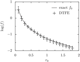
Figure 1: The DTFE-measured average phase-space density of the massive particles on surfaces where the exact phase-space density is constant. Each average phase-space density was calculated using 5,000 random points on the surface. The error-bars denote the Poissonian error which is typically 30%. However, the error in the average density itself is much smaller, typically about 7% and it never exceeds 10%.

4 Numerical Simulations

We used a large set of numerical simulations to measure $\left<K(S_{1},V_{0})\right>$ for 12 initial regions $V_{0}$ and 5 final surfaces $S_{1}$. All simulations used the same initial phase-space density $f_{0}(\mathbf{r},\mathbf{v})$ which was realised using 120,000 massive particles. Each of the initial $V_{0}$ regions was sampled using 100,000 test particles. The simulations were run in physical coordinates with no cosmological expansion and in dimensionless mode with the gravitational constant, unitlength, unitmass and unitvelocity all set to unity.

As was mentioned in Sec. 3.1, we used 5 different realisation of essentially the same simulation in order to estimate the sensitivity of the final $\left<K(S_{1},V_{0})\right>$ to a particular realisation. Therefore, for each $V_{0}$ we run a set of 5 different simulations in which we used a different realisation of $f_{0}(\mathbf{r},\mathbf{v})$ (by using a different random-number-generator seed in the routine that set the initial positions and velocities of the massive particles). The initial positions and velocities of the test particles in $V_{0}$ were always the same. Our results, which are presented in Sec. 5, are based on the average of these different realisations.

In the following sections we give a detailed description of the initial conditions and of the numerical simulations themselves.

4.1 Initial conditions

4.1.1 Massive particles

Initially, the system consisted of four identical haloes that collapse into each other, producing a single virialised halo. Each halo was realised using 30,000 massive particles, giving a total of 120,000 massive particles in each simulation. The haloes were placed in a symmetrical tetrahedron around the origin with their respective centres separated by six length units. This setup was chosen to maximise the level of violent relaxation and to ensure that there was no preferred direction in the final merger of the haloes. The test particles were then placed in equi-density regions inside each halo, as explained in the next section. A schematic picture of this setup is shown in Fig. 2: the four haloes are represented by the large spheres while the test particles are represented by the smaller spheres which are embedded inside them.

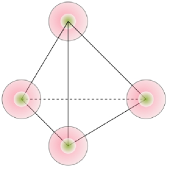
Figure 2: An illustration of our initial conditions showing the four haloes arranged in a symmetrical tetrahedron. The figure depicts the massive particles embedded with the massless test particles in the centre of each halo.

The haloes were set to be spherical and isotropic with Gaussian velocities:

$$f_{0}(\mathbf{r},\mathbf{v})=(2\pi)^{-3/2}\frac{\rho(r)}{\sigma^{3}(r)}e^{-\frac{v^{2}}{2\sigma^{2}(r)}}.$$ (33)

We used a Hernquist-like density profile

$$\rho(r)=\frac{1}{r(1+r)^{3}}\ ,$$ (34)

while the velocity dispersion $\sigma(r)$ was set by the Jeans equation (Binney & Tremaine, 1987) with a vanishing anisotropy parameter $\beta$

$$\frac{d(\rho\sigma_{r}^{2})}{dr}=-\rho\frac{d\Phi}{dr}\ .$$ (35)

This yielded

$$\sigma^{2}(r)=\frac{G}{\rho(r)}\int_{r}^{\infty}\frac{M(r^{\prime})\rho(r^{\prime})}{r^{\prime 2}}dr^{\prime}\ .$$ (36)

To increase the amount of violent relaxation in the simulations, we set the gravitational constant to $G=0.5$ in this calculation instead of the $G=1.0$ that was used in the simulation. This ensured that each halo would simultaneously collapse upon itself while merging with the other haloes.

$V_{0}(r_{0})$	$f_{0}$
$V_{0}(0.30)$	0.495881
$V_{0}(0.33)$	0.416877
$V_{0}(0.37)$	0.337873
$V_{0}(0.43)$	0.258869
$V_{0}(0.53)$	0.179865
$V_{0}(0.71)$	0.107462
$V_{0}(0.73)$	0.100861
$V_{0}(0.96)$	0.060260
$V_{0}(1.16)$	0.041870
$V_{0}(1.32)$	0.032079
$V_{0}(1.47)$	0.026000
$V_{0}(1.60)$	0.021858

Table 1: The phase-space density in the 12 initial volumes $V_{0}(r_{0})$. Each initial volume $V_{0}(r_{0})$ is a union of 4 shells around the 4 haloes. The outer radius of the shell is $r_{0}$ and the inner radius is $r_{0}/2$. The outer radius $r_{0}$ has values in the range $0.30<r_{0}<1.60$

4.1.2 Test particles

We used 12 initial $V_{0}$ regions. Each region was defined as the union of four identical thick shells in real space around each one of the 4 haloes. Each shell extended from the radius $r_{0}/2$ to $r_{0}$, with $r_{0}$ taking 12 possible values from 0.3 to 1.6. We denote the $V_{0}$ region that corresponds to $r_{0}$ by $V_{0}(r_{0})$. The initial values of $r_{0}$ and the corresponding $f_{0}$ for each $V_{0}$ are given in Table. 1.

We used 100,000 test particles to sample each $V_{0}$ region by placing 25,000 particles in every shell. The test particles were put in locations where the initial phase-space density Eq. (33) was exactly $f_{0}=(2\pi)^{-3/2}\rho(r_{0})/\sigma^{3}(r_{0})$. The position and velocity of a test particle were chosen in the following way: first we chose the particle position by randomly picking a location within the shell, in such a way that the real-space distribution of test particles would be homogeneous and isotropic. Once $\mathbf{r}$ was set it implied a value for $|\mathbf{v}|$ by requiring that the RHS of Eq. (33) would be equal to $f_{0}$. The directionality of $\mathbf{v}$ was then set isotropically.

Strictly speaking, one should add the contributions to $f(\mathbf{r},\mathbf{v})$ from the three other haloes. However, by taking $r_{0}$ small enough we have ensured that these contributions would never be larger than 10% of $f_{0}$.

4.2 The $S_{1}$ surfaces

The $S_{1}$ surfaces were chosen as two-dimensional shells in real space whose centres were at the centre of the equilibrium halo with radii of $r_{1}=0.3,0.4,0.5,0.6,0.7$. In accordance with Sec. 2.4, the measurements were done well within the centre of the relaxed halo where the dynamical time is short and violent relaxation is believed to be efficient, see Fig. 4 and Sec. 4.3 for more details. To specify a particular $S_{1}$ surface we use the notation $S_{1}(r_{1})$. We define the centre of the halo by calculating its centre of mass using an iterative centre of mass (COM) approach.

The velocity coordinates of the $S_{1}$ surfaces were chosen to be the velocity of the centre of mass, which amounts to $\mathbf{v}=0$ in the centre of mass frame. The underlying assumption here is that the equilibrium phase-space density of the test particles is isotropic when measured in that frame, and therefore for $\bar{\tau}=(\mathbf{r},\mathbf{v})$ the un-averaged (i.e., local) conditional probability is given by

$$K(\bar{\tau},\tau)=K\big{(}|\mathbf{r}|,|\mathbf{v}|,(\mathbf{r}\cdot\mathbf{v}),\tau\big{)}\ .$$ (37)

Such a function is constant over surfaces with $|\mathbf{r}|=r_{1}$ and $\mathbf{v}=0$. Support for this assumption is found in the Poissonian errors in $\left<K(S_{1},V_{0})\right>$ that we measured using the DTFE and Eq. (32). In all the measurements we obtained an error $\lesssim 30\%$ - which is the typical Poissonian error that was found when measuring the phase-space density in the spherical and isotropic Hernquist-like distribution in Eqs. (33-36) (see Fig. 1 and Sec. 3.2). If the phase-space density on these surfaces was not constant we would have obtained much larger errors.

4.3 $N$-body simulations and numerical effects

All simulations were run using the parallel version of the publicly available tree-code GADGET (Springel et al., 2001). The simulations were run on COSMOS, a shared-memory Altix 3700 with 152 1.3-GHz Itanium2 processors hosted at the Department of Applied Mathematics and Theoretical Physics (Cambridge).

The accuracy of a collisionless GADGET simulation can be determined by three parameters: the gravitational softening $\epsilon$, the internal time-step accuracy $\eta$ and the cell-opening accuracy parameter of the force calculation $\alpha$. After a number of test simulations we settled for the following values for the simulation parameters. We used a physically fixed force softening of $\epsilon=0.02$ for both the massive and massless test particles in the simulations. The half-mass radius $r_{m/2}$ of the final collapsed halo was $\sim 2.7$ length units and hence the employed softening was $\epsilon=7\times 10^{-3}r_{m/2}$. We chose timesteps according to $\Delta t=\sqrt{2\eta\epsilon/|\textbf{a}|}$ (time-step criterion 0 of GADGET). Here a is the acceleration and $\eta$ is the time-step accuracy parameter which we set to $\eta=0.01$. In the force calculation we employed the new GADGET cell opening criterion with a high force accuracy of $\alpha=0.001$, for details see Springel et al. (2001).

The simulations were ran for $t=70$ time units, with a typical run taking $\sim 70,000$ timesteps to reach the final time. In the final snapshot, at least 70% of the test particles were found within the half-mass radius, the fraction rising to above 90% for runs with low values of $r_{0}$. At the half-mass radius the crossing time was $t_{cross}\sim 10$, thus ensuring that the test particles that were used for the measurement were fully relaxed. Further support for this conclusion is presented in Fig. 3, which shows the virial ratio $-U/2K$ for one of the simulations. Here $U$ is the total potential energy and $K$ is the total kinetic energy of the system. For a fully relaxed system this ratio should be equal to one (the virial theorem). We see that the system fluctuates strongly until $t\sim 20$, after which the gravitational potential becomes constant and the evolution of the phase-space density (both of the massive and test particles) is through phase mixing only. Figure 4 shows the radial density profile of the massive particles at $t=70$. The dashed line is the function $4\rho_{0}(r)$ with $\rho_{0}(r)$ being the initial Hernquist-like profile of the four haloes given by Eq. (34). We see that the profile of the relaxed halo is well fitted by the profile of the initial haloes. This is in agreement with Boylan-Kolchin & Ma (2004) who found the same behaviour in a head-on collision of two cuspy haloes.

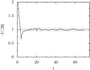
Figure 3: The virial ratio $-U/2K$ as a function of time for one of the simulations. $U$ is the total potential energy and $K$ is the total kinetic energy. Other simulations give very similar results. The dashed line denotes a ratio of 1 - for a fully relaxed system. For $t>30$ the virial ratio is always between $0.95$ and $1.05$, which are denoted by the dotted lines. The principal fluctuations occur at $t<20$, whereas at later times the gravitational potential is essentially constant and evolution proceeds through mixing.

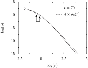
Figure 4: The radial density profile of the relaxed system (solid line) at $t=70$. The dashed line is the initial radial density profile of the 4 haloes scaled by a factor of 4. The good fit between the two is in agreement with other numerical experiments such as Boylan-Kolchin & Ma (2004). The two arrows denote the $r_{1}=0.3$ and $r_{1}=0.7$ radii which are the minimum and maximum radii at which the phase-space density of the test particles was measured.

An important test in assessing the reliability of a collisionless simulation is to calculate to what extent the simulation is affected by two-body relaxation. There have been a number of recent studies on what regions can be considered reliable against two-body relaxation [i.e. Power et al. (2003); Diemand et al. (2004)]. We chose here to follow Boylan-Kolchin & Ma (2004) who construct the local two-body relaxation time $t_{r}$ as defined in terms of the circular velocity $V_{circ}=V_{circ}(r)$, period $T(r)=2\pi r/V_{circ}$ and the number of particles $N$ (or equivalently mass $M$) interior to a radius r as

$$t_{r}(r) = T(r_{vir})\frac{N}{8\ln N}\frac{r}{r_{vir}}\frac{V_{circ}}{V_{circ}(r_{vir})}$$ (38)

$$= \frac{\pi}{4}\frac{N}{\ln N}\sqrt{\frac{r^{3}}{GM(r)}}.$$

To minimise the effects of two-body relaxation we require that $t_{r}(r)$ is longer than the overall simulation time for all values of $r$ for which we measure the conditional probabilities. We find for the range $r=0.3-0.7$ for which the measurement of the final phase-space density is done that the relaxation time is $t_{r}=90-470$, thus concluding that the simulation is not affected by two-body relaxation in our region of interest.

5 Results

Figure 5 shows $\log\left<K[S_{1}(r_{1}),V_{0}(r_{0})]\right>$ as a function of $r_{1}$ for 6 out of the 12 initial conditions, at two different times: $t_{1}=40$ time units and $t_{2}=70$ time units. To simplify the notation, we denote it simply by $K(r_{1},r_{0})$.

$K(r_{1},r_{0})$ is the result of averaging both over the $S_{1}(r_{1})$ surfaces and over the 5 different simulations that were run for each initial region $V_{0}(r_{0})$. We first calculated the $S_{1}$ average and then calculated the average of the different realisations. Both averages were done using $\log K$. In each realisation about 100-700 particles contributed to the $S_{1}(r_{1})$ average. These particles defined the Delaunay cells which were intersected by the 5D $S_{1}(r_{1})$ surface. The errors in Fig. 5 are the scatter errors among the different realisations. They are typically in the range $20\%-30\%$, and in general the two snapshots agree within that range. We also notice that for the lowest values of $r_{0}$ the agreement between the two snapshots is better than for higher values of $r_{0}$. This is an indication that the phase-space structure of the low $r_{0}$ test particles is more relaxed than that of the higher $r_{0}$. In addition, for lower values of $r_{0}$, the spatial distribution is more concentrated, having more test particles with smaller orbits. Such particles have shorter dynamical times and thus tend to relax more quickly than particles on outer orbits. It is therefore not surprising that $K(r_{1},r_{0})$ with lower $r_{0}$ are less fluctuating than those with higher values of $r_{0}$.

Figure 6 shows the log of the ratio $R(r_{i},r_{j})\equiv K(r_{i},r_{0})/K(r_{j},r_{0})$ calculated from the average $K(r,r_{0})$ at $t=70$. This is the main result of this paper. The upper plots show $\log R$ as a function of $f_{0}$ for comparison with the LB67 theory, whereas the lower plots show the same $\log R$ as a function of $1/f_{0}$ for comparison with the NK00 theory. In both groups the pairs $(r_{i},r_{j})$ are $(0.3,0.5)$, $(0.5,0.7)$ and $(0.3,0.7)$. Other combinations of radii give similar results.

In the upper plot we see that $\log R(r_{i},r_{j})$ increases until $f_{0}\sim 0.25$ after which it becomes approximately constant. On the other hand, in the lower plot $\log R(r_{i},r_{j})$ decreases until $1/f_{0}\sim 25$, where again it saturates. Putting it all together we see that $\log R(r_{i},r_{j})$ is approximately constant for $f_{0}<0.04$, then it increases (as a function of $f_{0}$) until $f_{0}\simeq 0.25$ and then it saturates once more. $\log R(r_{i},r_{j})$ is therefore highly non-linear both as a function of $f_{0}$ and as a function of $1/f_{0}$. As was discussed in Sec. 2.4, a linear behaviour is a necessary condition for either theories to be correct.

To quantify the above departure from non-linearity, we fitted a straight line for each of the size plots using a least-mean-square procedure. As expected, the results, are decisively against both theories. The quality of the fits is very bad, as can be clearly seen from the plots. The reduced $\chi^{2}$ of the fits for the Lynden-Bell theory are (left to right, top of Figure 6) $\chi_{LB}^{2}=1.31,2.51,6.59$ and for the Nakamura theory (left to right, bottom of Figure 6) $\chi_{NK}^{2}=4.06,2.43,10.00$. The lower $\chi^{2}$ for the first two fits is due to the small differences between $r_{i}$ and $r_{j}$, which causes $R_{ij}$ to be very close to unity and consequently $\log R_{ij}$ to approach zero, and thus be better approximated by a straight line. On the other hand, in the third pair where the difference between $r_{i}$ and $r_{j}$ is maximal, $R_{ij}$ spans a wider range of values, and consequently both theories produce a very poor fit of $\chi_{LB}^{2}=6.59$ and $\chi_{NK}^{2}=10.00$. This clearly shows that both theories fail miserably the test of linearity of $\log R$ in $f_{0}$ (LB67) and $1/f_{0}$ (NK00).

Figure 5: The average $\log K(r,r_{0})$ for 6 out of the 12 possible values of the initial radius $r_{0}$. The dashed line is the average at $t=40$ whereas the smooth line is the average at $t=70$. The average was calculated using 5 different runs of the same simulation with different realisations of the initial conditions. The statistical error is typically smaller than $20\%$. The agreement between the $t=40$ and $t=70$ snapshots is also typically within an error of $20\%$. It is particularly good for the lowest values of $r_{0}$, indicating that these test particles are more relaxed that the ones with larger values of $r_{0}$.

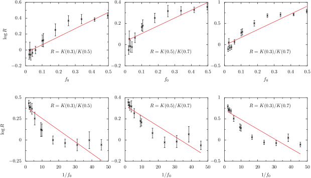
Figure 6: The logarithm of the ratio $R(r_{i},r_{j})\equiv K(r_{i},r_{0})/K(r_{j},r_{0})$ as a function of $f_{0}$ and of $1/f_{0}$, with $f_{0}$ being the initial phase-space density of the test particles. The $K(r_{j},r_{0})$ that was used to calculate the ratio is the average of 5 simulations, and is shown in Fig. 5. For all plots a straight line was fitted using a least-mean-square procedure. The resultant $\chi^{2}$ for the three upper plots (LB67) is (left to right) $\chi^{2}=1.31,2.51,6.59$ and for the lower plots (NK00) $\chi^{2}=4.06,2.43,10.00$. All plots show a very strong non-linear behaviour, in contradiction with both LB67 and NK00 theories.

6 Summary and conclusions

We have performed a series of $N$-body simulations to test the validity of the LB67 and NK00 theories. Unfortunately, due to a limited amount of time and computer resources we did not perform simulations with different $f_{0}(\mathbf{r},\mathbf{v})$ or with higher number of particles. Different initial conditions and different resolutions may yield qualitatively different equilibrium states [see, for example, Merrall & Henriksen (2003)]. The running of additional simulations is left for possible future work. However, in light of the strong non-linearity of the plots in Fig. 6, and the use of a very weak and general condition to test the theories, we believe that our conclusions will not be altered by additional simulations.

The main aspects in which our numerical experiment differ from previous studies are:

• We used 3D simulations whereas previous studies concentrated on 1D simulations.

• The experiment was explicitly designed to check which one of the two possible formulas of entropy is more correct: the LB67 formula which is derived using an equal-volume discretisation or the NK00 formula which is derived using an equal-mass discretisation.

• To distinguish between the two theories we used a very weak condition on the conditional probabilities $K_{i}(\tau)$, which was estimated by measuring the phase-space densities of sets of test particles. Therefore we did not need the full analytical solution of the theories with all its computational and conceptual difficulties.

• Previous attempts to verify the LB67 theory were done with the water-bucket initial conditions, in which the initial phase-space density has only one level. Here, as we needed to distinguish between the LB67 and NK00 theories, the initial phase-space density covered a continuous range.

The results of the experiment are summarised in Fig. 6. They provide very strong evidence against the LB67 and NK00 theories. As was discussed in Sec. 2.4, the linearity of $\log R$ in $f_{0}$ or $1/f_{0}$ is a very basic and weak requirement of both theories. Therefore the non-linearity of all the plots in Fig. 6 must be attributed to the failure of the most basic assumption in these theories, i.e., the maximisation of entropy. Indeed, we cannot explain the failure of the theories by the existence of additional conserved quantities that depend on the $f(\mathbf{r},\mathbf{v})$ (such as the total angular momentum vector $\mathbf{L}$) since we have used the final $f(\mathbf{r},\mathbf{v})$ itself as a constraint. We also cannot argue that our measurements reflect the incomplete relaxation of the outer parts of the system since they are done in the innermost parts of the system (less than $1/2r_{m/2}$) and in addition the linearity condition is independent of the full solution of the theories that assumes complete relaxation in all parts of the system. As was explained in Sec. 2.4, the weaker the condition is, the deeper is the failure of the theories if they do not pass it - and this is the bottom line.

In some respect this is a disappointing result as it shows that neither of the theories is even remotely correct. Additionally we are unable to decide which definition of the entropy is the “right” one as they both seem to perform equally bad.

On the other hand, one may find some sort of comfort in the fact that both theories fail, as there is no solid a priori theoretical argument against either equal-volume discretisation or equal-mass discretisation, and it is not obvious why they should produce such different results in the first place. Additionally, as was shown recently by Arad & Lynden-Bell (2005), both theories contain some sort of self-inconsistency since they are both non-transitive. Knowing that the theories are fundamentally wrong empirically thus solves many of these problems or at least makes them less relevant.

References

- Arad et al. (2004) Arad I., Dekel A., Klypin A., 2004, MNRAS, 353, 15
- Arad & Lynden-Bell (2005) Arad I., Lynden-Bell D., 2005, MNRAS, 361, 385
- Boylan-Kolchin & Ma (2004) Boylan-Kolchin M., Ma, C.-P., 2004, MNRAS, 349, 1117
- Binney & Tremaine (1987) Binney J., Tremaine S., 1987, Galactic Dynamics, Princeton Univ. Press, Princeton, NJ
- Chavanis (1998) Chavanis P.-H., 1998, MNRAS, 300, 981
- Cohen & Lecar (1968) Cohen L., Lecar M., 1968, MNRAS, 146, 161
- Cuperman at el. (1969) Cuperman S., Goldstein S., Lecar M., 1969, MNRAS, 146, 161
- Diemand et al. (2004) Diemand J., Moore B., Stadel J., Kazantzidis S., 2004, MNRAS, 348, 977
- Goldstein et al. (1969) Goldstein S., Cuperman S., Lecar M., 1969, MNRAS, 143, 209
- Jaynes (1957a) Jaynes E. T., 1957, Phys. Rev., 106, 620
- Jaynes (1957b) Jaynes E. T., 1957, Phys. Rev., 108, 171
- Hansen et al. (2005) Hansen S. S, Egli D., Hollenstein L., Salzmann C., 2005, New Astron, 10, 379
- Heggie (1991) Heggie D. C., 1991, in Roy A. E., ed., Predictability, Stability and Chaos in -Body Dynamical Systems. Plenum Press, New York, p. 47
- Hénon (1968) Hénon M., 1968, Bull. Astronomique, 3, 241
- Henriksen (2004) Henriksen R. N., 2004, MNRAS, 355, 1217
- Lecar & Cohen (1971) Lecar M., Cohen L., 1971, Astrophys. Space Sci., 13, 397
- Lynden-Bell (1967) Lynden-Bell D., 1967, MNRAS, 136, 101
- Kull et al. (1997) Kull A., Treumann R. A., Bohringer H, 1997, ApJ, 484, 58
- Merrall & Henriksen (2003) Merral T. E. C., Henriksen R. N., 2003, ApJ, 595, 43
- Moutarde et al (1995) Moutarde F., Alimi J. M., Bouchet F. R., Pellat R., 1995, ApJ, 441, 10
- Nakamura (2000) Nakamura T. K. 2000, ApJ, 531, 739
- Power et al. (2003) Power C., Navarro J.F., Jenkins A., Frenk C.S., White S.D.M., Springel V., Stadel J., Quinn T., 2003, MNRAS, 338, 14
- Quinlan & Tremaine (1992) Quinlan G. D., Tremaine S., 1992, MNRAS, 259, 505
- Schaap & van de Weygaert (2000) Schaap W., van de Weygaert R., 2000, A&A, 363, L29
- Shu (1978) Shu F. H, 1978, Apj, 255, 83
- Springel et al. (2001) Springel V., Yoshida N., White S.D.M., 2001, New Astron, 6, 79
- Spergel & Hernquist (1992) Spergel D. N, Hernquist L., 1992, ApJ, 75
- Stiavelli & Bertin (1987) Stiavelli M., Bertin G., 1987, MNRAS, 229, 61
- Tanekusa (1987) Tanekusa J., 1987, Publ. Astron. Soc. Japan, 39, 425
- Trenti & Bertin (2005) Trenti M., Bertin G., 2005, A&A, 429, 161