Elementary Heating Events - Magnetic Interactions Between Two Flux Sources. III Energy Considerations

The magnetic field plays a crucial role in heating the solar corona - this has been known for many years - but the exact energy release mechanism(s) is(are) still unknown. Here, we investigate in detail, using resistive, non-ideal, MHD models, the process of magnetic energy release in a situation where two initially independent flux systems are forced into each other. Work done by the foot point motions goes into building a current sheet in which magnetic reconnection releases some of the free magnetic energy leading to magnetic connectivity changes. The scaling relations of the energy input and output are determined as functions of the driving velocity and the strength of fluxes in the independent flux systems. In particular, it is found that the energy injected into the system is proportional to the distance travelled. Similarly, the rate of Joule dissipation is related to the distance travelled. Hence, rapidly driven foot points lead to bright, intense, but short-lived events, whilst slowly driven foot points produce weaker, but longer-lived brightenings. Integrated over the lifetime of the events both would produce the same heating if all other factors were the same. A strong overlying field has the effect of creating compact flux lobes from the sources. These appear to lead to a more rapid injection of energy, as well as a more rapid release of energy. Thus, the stronger the overlying field the more compact and more intense the heating. This means observers need to know not only the flux of the magnetic fragments involved in an event, but also their rate and direction of movement, as well as the strength and orientation of the surrounding field to be able to predict the energy dissipated. Furthermore, it is found that rough estimates of the available energy can be obtained from simple models, starting from initial potential situations, but that the time scale for the energy release and, therefore its impact on the coronal plasma, can only be determined from more detailed investigations of the non-ideal behaviour of the plasma.

1 Introduction

Discussions about the mechanism(s) that maintain the solar corona at temperatures in excess of a million degrees Kelvin have been going on since the late fifties. Much has been learnt, but the exact details of any mechanism are still not certain. The energy reservoir driving the heating has, for a long time, been believed to be the turbulent convection zone below the solar photosphere. Here, the magnetic field is, to a high degree, frozen into the plasma and turbulent velocity flows advect the embedded magnetic field. From the photosphere the magnetic field extends into the chromosphere and corona. Buffeting of the coronal field’s ‘foot points’ injects energy that propagates up along magnetic field lines into the corona. Here, somehow, it is released contributing to plasma heating, bulk plasma acceleration and localised particle acceleration.

Many mechanisms have been investigated and a general division of models, depending on the timescale of the imposed driver relative to the Alfvén crossing time of the magnetic structure, has been applied. Boundary motions changing faster than the Alfvén travel time correspond to the initiation of wave packages or trains (AC heating) that, to a certain degree, propagate along magnetic field lines and may release their energy through processes such as phase mixing or resonant absorption (e.g., Heyvaerts and Priest 1983 ; Goossens and Ruderman 1995 ; Goedbloed 1979 ; Ionson 1978 ). For long time-scale systematic driving periods (DC heating) changes in the magnetic field structure result in the build up of localised current sheets. These eventually dissipate through magnetic reconnection which changes the field line connectivity leading to the release of the stresses built up in the system (e.g., Parker 1972 ; Parker 1988 ; Heyvaerts and Priest 1984 ; van Ballegooijen 1986 ; Galsgaard and Nordlund 1996 ).

From small-scale energy release events in the solar atmosphere, such as “bright points” and “active-region transient brightenings” a scenario where the energy release is caused by magnetic flux cancellation or emergence has been suggested (e.g., Dreher et al.1997 ; Longcope 1998 ; Longcope et al. 2001 ; Mandrini et al. 1996 ; Parnell et al. 1994a ; Parnell et al. 1994b ; Parnell and Priest 1995 ; Priest et al. 1994 ; Shimizu et al. 1994 ). Due to the complexities of the magnetic carpet and the associated overlying magnetic field structure there is another, possibly more important, mechanism that has only recently been considered. In such a situation, the flux sources are not cancelled or emerged, but are simply advected past each other resulting in flux connectivity changes as their flux lobes, which extend into the corona, are forced into each other. Longcope 1998 investigated this scenario for two flux sources embedded in an overlying magnetic field using the minimum current corona approach and found that both the closing and the reopening of the magnetic flux occurs through separator reconnection. This process has further been analysed using a numerical approach to solve the non-ideal time dependent MHD equations (Galsgaard et al. 2000 ; Parnell and Galsgaard 2004 ).

In these two previous papers (Galsgaard et al. 2000 paper I and Parnell and Galsgaard 2004 paper II) different aspects of this type of interaction were investigated. Two initially independent flux systems lying in a horizontal uniform field were forced into each other by imposed boundary motions. The resulting dynamical interaction, described in paper I, revealed that there are two types of reconnection involved. First, the flux from the independent systems is connected through separator reconnection and later it is re-opened through the generally slower separatrix-surface reconnection. The reconnection rates of these processes were determined in Paper II as is their dependence on the direction of the overlying magnetic field with respect to the imposed driver.

In this paper, we investigate the energy dissipation in the same basic setup with particular attention paid to the effects of the driving velocity and the strength of the overlying magnetic field. This enables us to find scaling relations for the energy release in terms of these parameters. Such scalings are required to provide predictions of the energy release in similar individual events on the Sun. We also consider how variations in the driving velocity and field strength affect the reconnection rate providing further information necessary for determining the heating capability of such events. The structure of the paper is as follows. In Section 2, a brief description of the model is given. For completeness, Section 3 outlines the general dynamical evolution of the event, as discussed in detail in Papers I and II. In Section 4, the rates of reconnection and the connectivity changes in the models are compared. Section 5 discusses issues relating to the energetics of the experiments. Finally, Section 6, considers the implications of our findings.

2 Model

The setup used here is the same as that used in Papers I and II, where two localised magnetic sources of equal, but opposite, polarity flux are situated in a photospheric plane. From these a potential magnetic field is found numerically for a cubic domain with closed boundaries. This setup provides a dipole configuration with all the flux from the positive source connecting to the negative source. In our domain, which spans [0-1] in the $x$ and $y$ directions, the two sources are located at $(x,y)=(\frac{1}{3},\frac{1}{3})$ and $(x,y)=(\frac{2}{3},\frac{2}{3})$ on the $z=0$ boundary of the domain. The flux within the sources follows a $\frac{1}{2}(1+\cos(\pi r/R))$ distribution, where $r$ is the radius from the source centre and $R$ the maximum radius of the sources (in these experiments $R$ is 0.065 in units of the box). To break the connectivity of the sources a constant magnetic field, $B_{y}$, of sufficient strength and the correct sign, is added in the $y$ direction, thus rendering the two flux sources magnetically independent with their associated flux lobes running parallel to each other in the $y$ direction. Two 3D magnetic null points are created in the $z=0$ plane and are orientated in such a way that their spine axes lie in the $z=0$ plane, connecting each null with a single source, whilst their fan planes divide space into independent flux regions. The initial topology in the experiments (shown in Fig. 1) has three independent flux regions - two connected to the sources and one containing the overlying field.

Figure 1: An example of the initial conditions for the experiments. Magnetic field lines are traced revealing the fan separatrix surfaces which outline the independent flux lobes from the sources. The shaded regions on the bottom plane show the location and flux distribution of the magnetic sources. The arrows on the bottom boundary indicate the regions where the driving velocity is imposed.

The imposed driving in these experiments has the same form as that used in papers I and II, namely a piecewise uniform advection of the flux sources in the $x$ direction such that the independent flux regions are driven past each other, see Fig. 1. The velocity is imposed in two narrow regions on the $z=0$ boundary with sufficient width such that the sources are advected without changing shape. We are interested, here, in the dynamical evolution of the magnetic field and, therefore, we ignore the complicated structure of the solar atmosphere and instead consider, for simplicity, an isothermal, constant density atmosphere.

For numerical reasons, the closed box, which has no flux passing through the horizontal walls and is used to derive the initial potential magnetic field, is replaced by a domain with boundaries that are periodic in the horizontal directions (allowing flux through these walls) during the time dependent evolution of the system. We could have derived the initial potential magnetic field of such a 2D periodic configuration, but this has the disadvantage that the initial connectivity of the sources becomes much more complicated as they would be allowed to connect to other sources through all the periodic boundaries, as well as inside the domain. The disadvantage with having a change in boundary conditions between the initial and time dependent field is that the periodic (horizontal) sides of the box create a narrow layer where initial spurious current concentrations form and the condition $\nabla\cdot{\bf B}=0$ is not fulfilled. The currents initiate waves that propagate through the domain with time. Their amplitudes are insignificant compared to the dynamical response of the plasma to the advection of the two flux sources and have no implications on the evolution of the magnetic field. The regions where $\nabla\cdot{\bf B}\neq 0$ remain fixed and do not propagate through the domain so they cause no problems for the evolution of the magnetic field.

Two sets of experiments are investigated to better understand the energy release and reconnection processes as the sources are forced to pass each other. One set considers the implications of different driving speeds of the sources whilst the second allows the effects of varying the relative strengths of the flux sources with respect to the overlying field to be investigated. For the first set, the magnetic configuration is kept constant, but the driving velocity in the $z=0$ boundary is varied. In the second case, the strength of the overlying magnetic field in the $y$ direction is varied. To limit the number of experiments and to allow easy comparisons, the range of overlying field strengths are chosen such that initially the two sources are always totally unconnected. The minimum value of $B_{y}$ used is such that the flux lobes of the two sources are nearly touching in the $z=0$ plane. Similarly, the maximum value is chosen such that sufficient numerical resolution of the flux domains is maintained. Changing the $B_{y}$ component is equivalent to changing the length scale of the independent flux regions: as $B_{y}$ is increased the magnetic flux per unit area increases.

Table (1) shows the characteristic parameters of the experiments that are conducted, listing the imposed peak driving velocity $v_{d}$, the duration of driving $t_{d}$, the strength of $B_{y}$ and the numerical resolution (all parameters are given in units of the code).

Table 1: The characteristic parameters of the 8 experiments, giving the name, driving velocity and duration, the strength of the constant overlying magnetic field and the numerical resolution. Note, experiments $D2$ and $H2$ are the same.

Case	$v_{d}$	$t_{d}$	$B_{y}$	resolution
$D1$	0.0125	44	0.1	128x128x65
$D2$	0.025	22	0.1	128x128x65
$D3$	0.05	11	0.1	128x128x65
$D4$	0.025	-	0.1	128x128x65
$D5$	0.025	22	0.1	256x256x129
$H1$	0.025	22	0.076	128x128x65
$H2$	0.025	22	0.1	128x128x65
$H3$	0.025	22	0.2	128x128x65
$H4$	0.025	22	0.2	256x256x129

Together these experiments are designed to increase our insight into the dynamical interaction of magnetic flux systems and provide a basis for predicting energy release rates in similar events observed in the solar atmosphere.

3 Global Behaviour

For completeness a short description of the dynamical evolution of the magnetic field is given here; a more detail account of the evolution can be found in papers I and II. The dynamical evolution is followed by solving the time dependent, non-ideal, MHD equations numerically in a 3D Cartesian domain (for more details about the numerical approach see paper I and II and references their in).

The opposite polarity magnetic sources are advected by the imposed boundary flow and their flux lobes move towards each other. When the flux lobe from one source comes up against the other source, the flux lobe is lifted up over the moving source. This action leads to an interlocking of the flux lobes from the sources. Further advection of the sources creates forces on the intertwined flux lobes and a strong current builds up along the interface between them. This current is located along the separator line connecting the two magnetic null points which, due to the continued advection, collapses into a current sheet. When the current density becomes strong enough reconnection starts within this sheet rapidly changing the field line connectivity and allowing the two sources to connect. This process continues until the sources are well past the point of closest approach and a large fraction of the initially open flux is closed.

As the sources are advected even further apart an interface between the connected flux and the ambient open field creates a dome shaped separatrix surface upon which strong, some what irregular, current concentrations form. This current is a consequence of the rapid tangential change in orientation of the field lines across this surface and is associated with the reopening of the magnetic field connecting the two sources. When the driving is stopped, in general, only a fraction of the connected flux has re-opened and the opening rate decreases rapidly, requiring a long time to fully disconnect the two sources.

4 Connectivity Changes and Reconnection Rates

In this paper, we are interested in studying the energetics of simple magnetic interactions. In order to equate changes seen in the energetics of the experiments to physical changes in the system, we first discuss briefly the connectivity changes and rates of reconnection that occur. The results for the varying driving speed experiments are the same as those given in paper II, however, the varying overlying field strength experiments are all new.

4.1 Changes in Connectivity

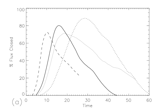
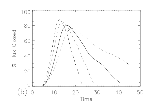
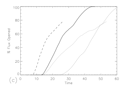
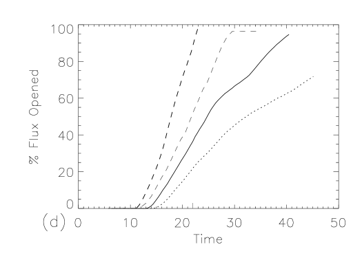
Figure 2: The percentage of (a & b) closed and (c & d) re-opened flux versus time. The graphs on the left refer to the varying driving speed experiments and those on the right to the varying overlying field strength experiments.

As in Paper II, the change in field line connectivity between the two sources is followed for each experiment. The graphs in Fig. 2 show the temporal evolution of the percentage of closed flux (top row) or percentage of re-opened flux (second row). The two left-hand graphs show the curves for the varying driving speed experiments whilst the right-hand ones show those with varying overlying field strength. In all experiments, the time is in numerical time units. The percentage of closed or re-opened flux for each source is found by identifying the endpoints of field lines (thin flux tubes) in exactly the same way as those in paper II. More than 12 500 flux tubes are tracked from each source at each time step with a maximum of 0.03 % of the total source flux in any one flux tube.

Although the two sources in each experiments are initially completely unconnected they all pass through a phase where they become increasing connected. Just before the amount of closed flux reaches its peaks, the first re-opened flux is generated. There are a number of points that can be noted from these graphs:

• The time of onset of closing the flux is dependent on the speed of driving (e.g., $t=8$, 5, 3 for $v_{d}=0.0125$, 0.025 and 0.05), but appears to be independent of the strength of the overlying field (e.g., $t=5$ for all $B_{y}$). Basically, the separator reconnection process which creates the closed field starts when sufficient stresses (currents) have developed between the two entwined flux lobes and, hence, is dependent on how far the flux lobes have moved. The dependence on the driving speed is therefore not surprising. Note, that the more slowly driven sources start to connect after a shorter distance has been travelled than the more quickly driven sources. This is due to the travel time of information in the domain which can respond relatively faster the more slowly it is driven. In the experiments with varying overlying field strength the sources start to connect at about the same time. At first sight this seems strange since the overlying field has the affect of decreasing the size of the flux lobes as its strength increases. Thus, for the same advection distance, the strongest overlying field experiments produces the least entwined flux lobes. However, this effect is counteracted by the fact that the flux density within the lobes is greater with higher $B_{y}$, leading to similar currents being generated and thus reconnection starting at about the same time in each experiment.

• The size and time of the peak closed flux is dependent on both the driving speed and the strength of the overlying field. The fastest driver and strongest overlying field both lead to the earliest peaks in closed flux. This is because in both cases they give rise to rapid reconnection since the fast driving and strong field maintain the stresses in the system. Note, however that the faster the driver the lower the peak in closed flux suggesting that the more rapid the reconnection the less complete it is. On the other hand the reconnection appears to be more complete for stronger $B_{y}$ leading to a greater peak in closed flux. The completeness of the reconnection process is determined by the relative speed of the driver to the Alfvén travel time in the system. In the fast driver case there is little time for the system to respond, however, in the strong $B_{y}$ case the Alfvén speed is greater and so the system has more time to respond.

• The start of the re-opening process (separatrix-surface reconnection) is affected by both $v_{d}$ and $B_{y}$. Again the more rapid the driver the earlier in time the re-opening starts, $t=25$, 14 and 8, respectively, for $v_{d}=0.0125$, 0.025 and 0.05. However, by comparing the advection distance instead it is the slowest driven case that starts to reopen at the shortest driven distance. It therefore also has the shortest advection distance between the onsets of the two classes of reconnection. The onset of reopening also depends on the overlying field strength, with the strongest $B_{y}$ seeing the first reopened flux. Thus, the system with the shortest Alfvén travel time (largest value of $B_{y}$) responds the fastest.

All the above points indicate that, of course, reconnection in a dynamical MHD situation is not rapid enough to process all the flux as soon as it is advected into the current sheet, as would happen through equi-potential evolution.

In the classical 2D reconnection scenarios (Sweet 1958 ; Parker 1957 ; Petschek 1964 ) the reconnection rate scales inversely as some function of the magnetic Reynolds number. The reconnection rate can therefore be changed by changing any of the three parameters defining the Reynolds number. For instance, increasing the coronal field strength leads to a decrease in the length of the current sheet and, hence, an increase in the reconnection rate (assuming this is the only parameter changing). However, from Fig. 2, it is seen that in the 3D numerical experiments the situation is more complicated than this. An increase in overlying magnetic field strength not only leads to a decrease in width of the current sheet (Note, in three-dimensions, a current sheet typically has dimensions thickness $<<$ width $<<$ length, as seen in Fig. 2 (Parnell and Galsgaard 2004 ) and so for the local magnetic Reynolds number what is important is the width of the current sheet), but also results in an increase in the local Alfvén speed in the vicinity of the reconnection site. Since two factors have now changed the resulting change in the rate of reconnection is not clear and a priori cannot be predicted. In fact, it seems that an increase in overlying field strength leads to an increase in reconnection rate. Further, increasing the numerical resolution, effectively decreases $\eta$ and subsequently the reconnection speed. Due to the multiple effects of changing a single parameter in the experiments it is not simple to predict what would happen as various parameters are changed. Instead, by obtaining the magnetic Reynolds numbers for each experiment it is possible to show that the behaviour follows the classical trend, with a decreasing reconnection rate for increasing $R_{m}$.

The effect of higher resolution leading to delayed and slightly slower reconnection is again seen by comparing $D5$, a high resolution run with $D2$ its lower resolution counterpart. Otherwise these two runs are essentially the same.

4.2 Reconnection Rates

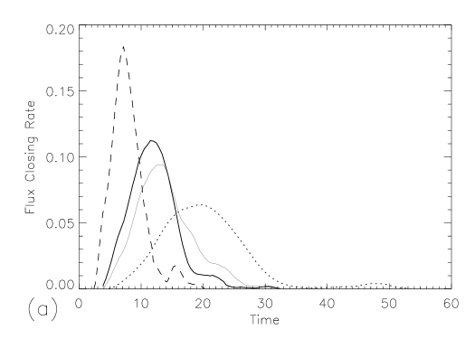
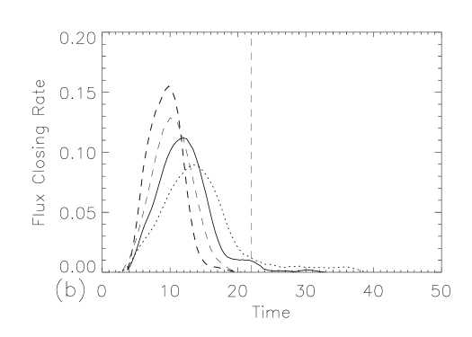
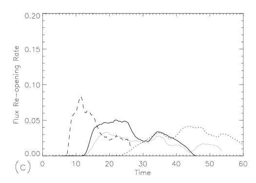
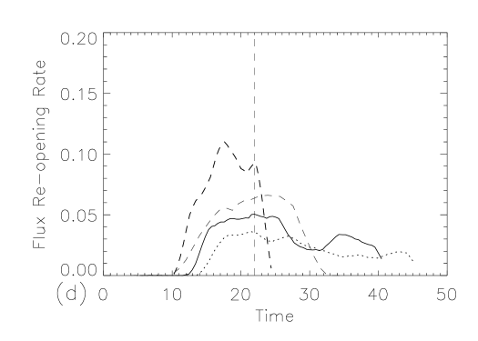
Figure 3: The reconnection rate of (a & b) closing and (c & d) opening the field. The left-hand graphs refer to the varying driving speed experiments and those on the right to the varying overlying field strength experiments.

The two rows of graphs in Fig. 3 show the temporal evolution of the separator (closing) and separatrix-surface (opening) reconnection rates, respectively. With, as before, the varying driving speed results on the left and the varying overlying field results on the right. The rates of reconnection have been determined in exactly the same way as those in paper II, i.e., from differentiation of the flux closing and re-opening curves. From these graphs it is clear that the peak rate of closing or opening the field is dependent on the speed of the drivers. From paper II the following formulae were determined relating driving speed ($v_{d}$) and overlying field angle ($\theta$ - here $\theta=0$) to peak closing ($R_{cmx}$) or re-opening ($R_{omx}$) reconnection rates:

$$R_{cmx}=\frac{0.44v_{d}\cos\theta}{v_{d}\cos\theta+0.08},\hskip 14.22636pt{\rm and}\hskip 14.22636ptR_{omx}=\frac{0.19v_{d}\cos\theta}{v_{d}\cos\theta+0.06},$$

where in these formulae the driving speed and peak rates of reconnection are normalised with respect to the peak Alfvén velocity in the sources. Thus, the peak rates of separator reconnection are about twice the peak rates of separatrix-surface reconnection. Moreover, it was found that, at the typical observed driving speed of fragments in the photosphere (i.e., a hundredth of the Alfvén speed) the peak rate of separator reconnection was 58% of the instantaneous reconnection rate (determined from the evolution of an equi-potential model) and the separatrix-surface reconnection rate was 29%. Thus, both the separator and separatrix-surface reconnection rates are fast.

The reconnection rates also vary for varying overlying field strength. There are two effects that are at work in these experiments. Varying the overlying field leads to (i) changes in the size of the flux lobes and, therefore, changes in the flux per unit area (a real physical effect), and (ii) changing the size of the flux lobes has the knock on effect of changing the resolution across the lobe and, hence, changing the resistivity of the experiment (a numerical artifact). Separating these two effects is not straight forward and so determining exactly how the rate of reconnection scales with $B_{y}$ is not clear. Neither is the significance of the effect.

5 Energetics

Here, we investigate the energetics of the different scenarios given in Table (1). In particular, we are interested in the balance between the energy input, the energy growth, and its release through viscous and resistive processes.

5.1 Effects of the Driving Velocity

First, we discuss the impact of the driving velocity on the energetics of the system. To make comparisons between the experiments easier, the time scales of the experiments are scaled to fit that of experiment $D2$ such that the sources cover the same distance in the same time (i.e., one could consider that they have been plotted against driving distance rather than time). This scaling is only applied to the various parameters up until the driver is switched off, after which the parameters are all plotted against their true numerical time. Clearly, where the times are scaled the time dependent variables, such as the Poynting flux and the dissipation rates, must also be scaled accordingly, but no changes need be made to the volume energy parameters.

5.1.1 Poynting Flux

Figure 4: The scaled Poynting flux for the experiments, $D1$-$D5$, as a function of scaled time. The imposed driving velocities are 0.0125 (dotted line - $D1$), 0.025 (thick solid line - $D2$, thin solid line $D5$ and dot-dashed line $D4$) and 0.05 (dashed line - $D3$). The vertical dashed line is the time at which all drivers are switched off except for $D4$ which is driven continuously. $D5$ has higher numerical resolution than all the other experiments.

Fig. 4 shows the Poynting flux for the five experiments, $D1$-$D5$, which are all scaled to the same advection distance as that used in experiment $D2$ for comparison. This requires multiplication by a factor of 2 and 0.5, respectively, to the actual Poynting fluxes of experiments $D1$ and $D3$. Clearly, all the experiments have very similar scaled Poynting fluxes which show an almost linear, growth in time up until the switching off of the drivers. The undulations in the curves simply correspond to the Alfvén travel time across the periodic domain. It is only towards the end of the driving period that a turn over in the Poynting flux is found in the slowest driven experiment $D1$ and also possibly in $D2$. There is little difference between $D2$ and $D5$, which have the same driving velocity, but a different numerical resolution.

The three curves $D1$-$D3$ represent changes in driving velocity with a factor of 2 between each one. So why, when scaled to the same time frame, do they show almost the same linear growth with time? Also why are there offsets in the initial Poynting flux values? These questions can be answered by looking at the expressions for the induction equation and the Poynting flux.

Consider the ideal induction equation with velocity simply in the $x$ direction, ${\bf u}=(u_{x},0,0)$. The resulting changes in the magnetic field, ${\bf B}=(B_{x},B_{y},B_{z})$, on the driving boundary are given by

$${{\partial{\bf B}}\over{\partial t}}=\left({{\partial}\over{\partial y}}(u_{x}B_{y})+{{\partial}\over{\partial z}}(u_{x}B_{z}),-{{\partial}\over{\partial x}}(u_{x}B_{y}),-{{\partial}\over{\partial x}}(u_{x}B_{z})\right).$$ (1)

Assuming that (i) the magnetic field is directed into the domain, (ii) $u_{x}$ is in the positive $x$ direction (iii) both the magnitudes of ${\bf B}$ and ${\bf u}$ decrease with height (i.e., increasing $z$) and (iv) both ${\bf B}$ and ${\bf u}$ have only a weak $y$ dependence, then $B_{x}$ will have a negative growth in height above the driving boundary surface. At the same time both $B_{y}$ and $B_{z}$ are advected with the flow, maintaining their spatial structure. This indicates that the magnetic field lines that thread the driving boundary (i.e., the magnetic field lines from the sources) lag behind their foot points as they are driven across the box resulting in a change in the angle of the magnetic field in the $xz$ plane as time progresses. Furthermore, assuming that (i) the driving velocity is slow relative to the Alfvén speed and (ii) the time since the driving started is short in comparison to the Alfvén time of the advected field lines, then the ratio of the driving velocity to the Alfvén velocity determines the maximum angle of the advected magnetic field lines to the surface normal, $\phi=\mbox{arctan}(v_{d}/v_{A})$. Now the Poynting flux injected by the driving is

$$P_{f}={1\over\mu}\int({\bf u}\times{\bf B})\times{\bf B}\cdot\bf{dS},$$ (2)

where ${\bf u}$ is the velocity on the boundary surface, $S$, and ${\bf B}$ is the magnetic field. Here, $S$ is the constant $z=0$ surface and, as indicated above, the velocity is in the $x$-direction only, thus Eq. (2) reduces to

$$P_{f}={1\over\mu}\int\int u_{x}B_{x}B_{z}dxdy.$$ (3)

Hence, the Poynting flux is fixed at a constant level proportional to $\phi$.

In the alternative case, where the driving velocity is also slow, but the time since the start of the driving is long in comparison to the Alfvén crossing times of the advected field lines, the angle $\phi$ grows linearly with time as the foot points are constantly advected in a systematic direction and the Poynting flux grows linearly with time (as already pointed out by Parker 1987 ; Galsgaard and Nordlund 1996 ).

In the present situation, neither of these two extremes fully applies, however, the near-linear growth of the Poynting flux in Fig. 4 suggests that the situation here is closest to the latter case. The reason for this may lie in the fact that the two flux lobes from the sources are soon forced into each other effectively fixing the ‘free’ ends of the field lines thus resulting in short field lines. Or it may be because of the rapid change in magnetic field strength as one moves away from the sources resulting in a decrease in the Alfvén velocity and hence, a slowing down of the propagation speed of information.

By assuming that the $x$ component of the induction equation is only weakly dependent on $y$, the value of $B_{x}$ can be approximated by,

$$B_{x}(t_{d})={\partial\over{\partial z}}(u_{x}B_{z})t_{d}\approx{{u_{x}B_{z}t_{d}}\over L},$$ (4)

where $L$ is the distance to the (apparent) end points of the field lines and $t_{d}$ is the time since the driving started. Substituting this into Eq. (3) leads to the following expression for the average Poynting flux input through $S$,

$$P_{f}\approx{1\over\mu}\int\int{{B_{z}^{2}u_{x}^{2}t_{d}}\over L}dxdy.$$ (5)

Assuming that $L$ and $B_{z}$ are close to constant in all the experiments, implies that changes in driving velocity and driving time lead to a simple scaling of the different cases. Namely, a doubling of the velocity increases the Poynting flux by a factor of 2 at the same shear distance. Hence, the re-scaling of the experiments for the graphs produces almost identical values for the experiments. The turn over of the Poynting flux in $D1$ indicates where the above approximation breaks down and a new regime starts.

The differences in Poynting flux seen in the initial phases of the experiments are effectively maintained throughout the driving period. Clearly, at the start, the Poynting flux is zero in every experiment, but when the driving is switched on there is a discontinuous jump. The level of the jump depends on the ratio of the driving and Alfvén velocities. This ratio is proportional to the ratio of $B_{x}$ and $B_{z}$, which shows that $B_{x}$ is proportional to the driving velocity in this regime. Substituting this into Eq.(3) one gets,

$$P_{f}\approx{{B_{z}^{2}u_{x}^{2}}\over{\mu u_{A}}}.$$ (6)

where $u_{A}$ is the Alfvén velocity. Doubling the driving velocity quadruples the Poynting flux which, with re-scaling, results in a doubling of the initial jump in Poynting flux, as seen in Fig. 4.

In Fig. 4, the continuously driven experiment $D4$ is clearly identifiably as the dot-dashed line that extends from the solid line of $D1$. Here, the initial linear growth is replaced with a more constant energy input after t = 22 with some fluctuations in time. This implies that even after the flux sources have passed each other a significant amount of energy continues to be injected through the driving process. This has similarities to the results that Galsgaard and Nordlund 1996 found in their experiments investigating flux braiding. In their scenario, an initial straight magnetic field was braided by a sequence of incompressible shear motions and after a few shear events a similar fluctuating input level, as seen here in $D4$, was obtained. Obviously, though here in $D4$, to accommodate such a sustained driving period, the sources are driven out of the box and back in the opposite side (since the side boundaries are periodic). Thus, interpretation of the results is not straight forward.

5.1.2 Magnetic and Kinetic Energy

Figure 5: (a) The ‘free’ magnetic energy (magnetic energy minus the potential energy) and (b) the kinetic energy for $D1$-$D5$ as a function of scaled time for t$<$22 and as a function of the correct time for t$>$22. The velocities are 0.0125 (dotted line - $D1$), 0.025 (thick solid line - $D2$, thin solid line $D5$ and dot-dashed line $D4$) and 0.05 (dashed line - $D3$). The grey vertical dashed line indicates when the driving velocity is switched off in all experiments except $D4$.

The evolution of the total magnetic and kinetic energy is shown in Fig. 5 for each experiment $D1$-$D5$. In Fig. 5a, the magnetic energy relative to the potential energy, as a function of scaled time, is plotted; this is effectively the ‘free’ magnetic energy in the system. Clearly, this energy increases in time throughout the driving period of the experiments with the rate of energy growth increasing with increasing driving velocity. Interestingly, the free magnetic energy shows no significant features that indicate the onset of separator reconnection (closing the field) or separatrix-surface reconnection (re-opening the field). This suggests that the injection of magnetic energy through driving the field is more dominant than the dissipation of the magnetic energy through reconnection.

Unsurprisingly, the kinetic energy also scales with driving velocity, however, here there are pronounced differences between the experiments (Fig. 5b). Unlike the magnetic energy, the kinetic energy initially rises before levelling off and then varies, with only small fluctuations, until the end of the driving. The time of levelling off gets later, by a factor of two, as the driving speed doubles, indicating that its onset is related to the travel time of information through the domain (the times of levelling represent the same absolute time in non-scaled time units). Note, that in the higher resolution experiment $D5$ the kinetic energy levels off at a higher value than in $D2$. This is due to the higher velocities that can be achieved following the formation of narrower current sheets in the high resolution experiment.

By comparing the two graphs in Fig. 5 it is clear that the maximum total kinetic energy in any one experiment is an order of magnitude smaller than the corresponding magnetic energy. This implies that the kinetic energy does not contribute significantly to the heating of the plasma through viscous dissipation. Instead, the near constant kinetic energy for the latter part of the driving period indicates that there is an equipartition between the energy input from magnetic forces and that lost through viscous dissipation.

Integrating Eq. (5) from $t=0$ to $t=t_{d}$ suggests that all experiments should be injected with the same energy under the assumptions assumed to derive Eq. (5), but this is clearly not true. There are three reasons why this is so. First, as seen in Fig. 4, the energy input increases with driving velocity due, basically, to the differences in the Poynting fluxes at the onset of driving. Second, the faster the driver, the shorter the time available for dissipation and the transfer of energy from magnetic to kinetic. Third, the more quickly driven experiments have a greater angle $\phi$ between the field lines and the surface normal as information has less time to propagate into the domain resulting in a slower dissipation rate. Thus, the more quickly driven experiments have a some what larger build up in magnetic energy.

The curves that continuously rise in both Fig. 5 graphs are, of course, related to $D4$ and show that continuous driving leads to continual energy injection into the domain. This implies that there is still a long way to go before a time averaged balance is reached between the Poynting flux, the dissipation and the conversion of magnetic energy into kinetic energy. In $D4$ the magnetic energy continues to increase smoothly until at least t=120 when the experiment is stopped. The kinetic energy also increases throughout this time, but in a stepwise fashion. This is due to the fact that the sources are driven many times across the box resulting in the closing and opening of the fluxes multiple times during the run with each time more kinetic energy being built up in the system.

Increasing the numerical resolution increases the ‘free’ magnetic energy in the system, because of a decrease in the joule dissipation following the associated decrease in magnetic resistivity (seen in the following section).

To get an idea about the decay times for the various experiments, no scalings are applied to the time axes for $t>t_{d}$. The decay curves for the magnetic energy show that the more free energy there is available, the faster it decays. They also indicate that the experiments all relax to quasi-static states that have approximately the same energy — just over 107% of the initial magnetic energy in the system. This implies that (i) the rate of magnetic dissipation tends to zero for large times and that (ii) a new force-free topology is found which is clearly different from both the initial potential configuration and the equivalent configuration found after the potential evolution of the field. This higher energy level state is a consequence of the increase in magnetic helicity in the numerical experiments during the advection of the sources; a helical structure is clearly visible within the closed field region of each of the experiments. Such a twist can not be found in the comparable potential solutions of the time dependent problem. Therefore, since dissipation of helicity, in general, takes place on a longer time scale than magnetic dissipation (Berger 1984 ) the energy of the magnetic field after the driving has stopped is naturally higher than before the driving was initiated.

The decay in the kinetic energy behaves in a similar manner to that of the magnetic energy in that, after the drivers are switched off, the fall off in kinetic energy is greatest for the experiment with the largest kinetic energy. Here, of course, it is expected that the kinetic energy will eventually drop to zero, the level it started at.

5.1.3 Joule versus Viscous Dissipation

Figure 6: (a) and (c) The scaled Joule and viscous dissipation, respectively, as a function of scaled time for $D1$-$D5$ up until the driver is stopped at $t=t_{d}$. (b) and (d) The correct Joule and viscous dissipation, respectively, but with the time scaled for $t<t_{d}$ and with correct time scales after $t=t_{d}$. The velocities are 0.0125 (dotted line $D1$), 0.025 (thick solid line $D2$, thin solid line $D5$ and dot-dashed line $D4$) and 0.05 (dashed line $D3$.)

As already suggested, joule dissipation is likely to dominate viscous dissipation. Fig. 6, which shows the scaled joule and viscous dissipation up until the drivers are switched off in the two left-hand graphs, confirms this with the dissipation due to ohmic heating some 50-100 times more effective that that due to viscous effects. Fig. 6a shows that three of the experiments, $D1$-$D3$, have almost identical scaled joule dissipation rates that increase linearly up to t=10. At $t=10$, $D1$, the most slowly driven case, then diverges from this linear regime with the other two cases following suit with delays of about two scaled-time units per increase in driving velocity. The times of these changes are comparable to the time at which about half of the flux between the two sources becomes connected (see Section (4) for a detailed discussion of the changes in connectivity) and the current in the separator current sheet starts to slowly decrease. These three experiments then have a period of fairly constant dissipation, lasting about 4-5 scaled-time units, before once again increasing. This second increase in dissipation relates to the re-opening of the magnetic flux through separatrix-surface reconnection (again see Section (4) for further details).

The viscous dissipation curves (Fig. 6c) also all start off with a similar linear growth rate, but they diverge from this after approximately one Alfvén time. Each curve then peaks at about the time the joule dissipation curves first break from their initial linear regime. Thus, these peaks are related to the closing of the field which results in highly localised velocity structures from the strongly driven separator reconnection. After the peaking the viscous dissipation rates either level off or drop, although their behaviour is not completely clear. There is no obvious counter part to the re-opening process, which is observed in the joule dissipation curves as a second rise phase. This is rather surprising and is likely to be related to the fact that the re-opening process occurs through weakly driven separatrix-surface reconnection which produces diffuse velocity structures.

Integrating the total joule dissipation from the start to the end of the driving gives close to the same value for experiments $D1-D3$. This indicates that approximately the same amount of energy is available for heating the plasma independent of the speed at which the sources are driven. This is not that surprising since in each case one would expect the same amount of flux to close and re-open and it relates well to the first-order assumption of the integrated energy input being independent of the rate of driving. Thus the heating essentially depends on the duration of the energy release process. If effects such as anisotropic heat conduction and optically thin radiation are ignored then the plasma heating rate would, to a first approximation, scale inversely with the duration time of the event.

The right-hand graphs in Fig. 6 show the unscaled joule and viscous dissipation rates against scaled time for $t<t_{d}$ and unscaled time for $t>t_{d}$. The joule dissipation curves (Fig. 6b) reveal that the most rapidly driven case naturally has a much higher rate of dissipation than the slower cases. Indeed, there is roughly a factor of 2 increase in rate for each doubling in driving speed. After the driving is stopped the joule dissipation rapidly decreases with the decay rate scaling with the driving speed. It is clear that the rates of joule dissipation in the $D1$-$D3$ experiments all decay to zero after about the same time. This is consistent with the evolution of the magnetic energy discussed earlier which approaches a new constant level towards the end of the experiments. The time scale for this to occur is short relative to large-scale magnetic diffusion. From the traditional diffusion equation, one might expect an exponential decay of the dissipation, but the decay curves are more reminiscent of a series of near linear decay periods changing at regular intervals of approximately twice the crossing time for the domain. The rapid decay of the dissipation is due to the diffusivity used in the numerical code, which has contributions from both a 2nd and 4th order diffusion operator implemented to stabilise the high-order finite-difference scheme. The high-order diffusivity acts efficiently on length scales close to the resolution limit, whilst length scales much longer than the resolution limit feel very little dissipation. This allows for the possibility that large-scale current structures can maintain their strength almost unaffected by dissipation.

The curves in Fig. 6d are the viscous dissipation counter parts of those in Fig. 6b. and they behave in a similar fashion with experiment $D3$ naturally having a much higher viscous dissipation rate than the other cases. All the viscous dissipation rates tend to zero at the end of the experiments with the dissipation in $D3$ falling off fastest. The decay of the viscous dissipation rates is consistent with the very low kinetic energies seen at the end of all the experiments.

Once again experiment $D4$ is clearly visible as having the only curves in Figs 6b and 6d that continue to increase after the driving has stopped for the other experiments. These curves show both that joule and viscous dissipation is maintained, despite significant fluctuations, whilst driving continues. It is most likely that the fluctuations are related to the changes in reconnection that occur due to the crossing of the periodic boundaries, although this is not easy to follow.

5.1.4 Peak Flow Velocities

Figure 7: The time evolution of the absolute values of the maximum (solid) and minimum (dotted) velocities in the (a) $x$, (b) $y$ and (c) $z$ directions of the $y=0$-plane half way between the driving boundaries for experiment $D2$ which has a driving velocity of $0.025$.

Finally, we investigate the temporal variations in the maximum and minimum flow velocities of the $y=0$-plane half way between the sources (i.e., in the vertical plane perpendicular to the direction of driving). The evolution of all the experiments follows the same pattern, thus we limit our discussion to just experiment $D2$. Fig. 7 shows the extremes of the three velocity components as functions of time. Three significant features are noted. Firstly, the $z$ velocity (Fig. 7c) shows a clear broad peak in maximum and minimum velocity followed by a period at a constant low level. Secondly, both the $x$ and $y$ velocities (Fig. 7a,b) show an even broader peak in their maximum/minimum values starting after the peak in the $z$ component. Thirdly, all components eventually level out to, or decrease to, a low, almost identical, constant velocity after a period of time. Comparing the evolution of these maximum/minimum velocity curves with the temporal evolution of the field line connectivity reveals clear correlations. The peaks in the $z$ velocity components relate to the initial closing of flux in which the two flux lobes start to interact. Thus, the peak $z$ velocities are most likely the outflows from the separator reconnection suggesting that there are two oppositely directed jets with almost the same maximum velocity. These reconnection jets cease to be important contributers to the plasma dynamics at about the time when the closed flux peaks indicating that there is a strong decline in the closing process after this. This feature is clearly evident in all experiments, independent of the driving speed.

The structure of the $x$ and $y$ velocity components vary much more between the experiments. These velocities are related to the re-opening of the closed magnetic field and represent the mainly horizontal outflow velocities associated with this process. Finally, a low level velocity state is reached for all the velocity components once the process of re-opening the flux ceases through lack of driving.

From the point of view of scalings it is found that the absolute peak $z$ velocity, $v_{zmx}$, increases with increasing driving velocity at a rate that is slower than the square root of the driving velocity (see Table (2)). However, the exact nature of this scaling relation is not known.

Table 2: The absolute peak $z$ velocity, $v_{zmx}$, for the four experiments

	$D1$	$D2$	$D3$	$D5$
$v_{d}$	0.0125	0.025	0.05	0.025
$v_{zmx}$	0.067	0.11	0.15	0.16

5.2 Effects of the Strength of the Overlying Magnetic Field

In this section, we investigate the effects on the energy release of having different strengths of overlying magnetic field in the same magnetically interacting system as above. Changing the field strength is equivalent to varying the flux from the sources and, hence, to varying the size of the flux lobes. The stronger the overlying field the smaller the flux lobes and the more rigid their advection. Clearly, this results in a smaller region of the system being directly influenced by the advection of the sources. Predictions of the behaviour of the various physical quantities are, therefore, not straight forward and we conduct the following numerical experiments to try and determine the possible scaling relations.

Four experiments, labelled $H1$-$H4$, are carried out with the first three ($H1$-$H3$) having overlying field strengths of $B_{y}=0.076$, $B_{y}=0.1$ and $B_{y}=0.2$, respectively. Experiment $H4$ is the same as $H3$ except it has double the numerical resolution. In all cases, the driving velocity and peak source strengths are the same (See Table 1 for details). Note, also that experiments $D2$ and $H2$ are the same. Here, since the driving velocity is the same in each experiment, there is no need to scale any of the results to different time frames, so no scalings are applied.

5.2.1 Poynting Flux

Figure 8: Poynting flux variations in time for experiments $H1$-$H4$. The different field strengths are $B_{y}=0.076$ ($H1$ - dotted), $B_{y}=0.1$ ($H2$ - solid black) and $B_{y}=0.2$ ($H3$ - thick dashed and $H4$ - thin dashed).

Varying the strength of the overlying field clearly has an affect on the Poynting flux (Fig. 8) which is anticipated since, from Eq. (1), it is apparent that increasing the strength of $B_{y}$ can change the growth rate of $B_{x}$, and this in turn effects the Poynting flux (Eq. (3)). This effect, however, only kicks in after one Alfvén crossing time (approximately, 5 time units), implying that $u_{x}$ has only a small variation in the $y$-direction at the driving boundary - this is not a surprise considering the imposed driving profile.

After t=5, the Poynting flux increases. This increase in Poynting flux is triggered by the crossing of the domain by the wave front created by the initial ramp up of the driving velocity. The stronger the overlying field, the smaller the source flux lobes, and although the region affected by the wave fronts is smaller their effect is greater. Thus, the effect on the local field lines from the wave interaction increases with increasing $B_{y}$. Hence, experiment $H3$, which has the strongest overlying field, has the fastest growth in Poynting flux. Furthermore, $H4$, which has a higher numerical resolution and therefore less numerical diffusion than $H3$, has a larger Poynting flux than $H3$, because it produces greater changes in the field line orientation.

For experiments $H1$ and $H2$, the increase in Poynting flux continues until the driving is stopped at t=22, but for $H3$ and $H4$, the growth in Poynting flux peaks at t=16 and t=18, respectively. The decline seen in $H3$ and $H4$ occurs because these experiments show a faster restructuring of the magnetic field to a lower energy state (more rapid release in magnetic energy) than the two other experiments giving rise to the early decay in Poynting flux.

This implies that making simple predictions about any scaling is difficult as it depends on the detailed structures of the magnetic field topology and velocity driving profile at any one time. Determining the overall magnetic topology is relatively straight forward, but the detailed small-scale variations in the magnetic field are not so easy to understand and yet they may be more important. Similarly, mean flow patterns created by the driving profile may be determined, but with addition of local variations means large errors may arise in estimates of the Poynting flux for real situations.

5.2.2 Magnetic and Kinetic Energy

Figure 9: (a) The ’free’ magnetic energy and (b) the kinetic energy for experiments $H1$-$H4$. The field strengths are $B_{y}$=0.076 ($H1$ - dotted), $B_{y}$=0.1 ($H2$ solid) and $B_{y}$=0.2 ($H3$ - thick dashed and $H4$ - thin dashed). The vertical dotted line denotes when the driver is switched off.

Naturally, increasing the strength of the overlying field increases the total magnetic energy in the system. It also increases the amount of ‘free’ magnetic energy (i.e., magnetic energy minus the potential magnetic energy) available at any time (Fig. 9a). The difference in ‘free’ magnetic energy between all the experiments only becomes apparent after one Alfvén crossing time as this is when the Poynting flux curves start to diverge. $H3$ and $H4$ clearly have a much larger gain in magnetic energy than the other experiments, as one might expect from their increased injection of Poynting flux. Note, though, that the ‘free’ magnetic energy for $H3$ starts to decrease at t=19, which is shortly after the time at which the Poynting flux starts to decrease. In comparison, the ‘free’ magnetic energy of the high resolution run, $H4$, continues to increase until the driving is turned off and does not follow the early decline that its Poynting flux has.

After the driving has stopped, the magnetic energy decreases for all experiments, with the most rapid decline seen in $H3$. The reason for the different rates of magnetic energy decline from experiments $H1$ to $H3$ is, in part, related to the relative decrease in numerical resolution of the flux lobes as the overlying field strength increases. $H3$ shows stronger local currents coupled with a smaller spatial resolution leading to a faster numerical dissipation of the currents in the system and, therefore, a more rapid decrease in the ‘free’ magnetic energy. This is confirmed by comparing the results from $H3$ and $H4$. The decay rates in these two experiments look similar, but the high resolution experiment is capable of maintaining a higher ‘free’ magnetic energy than the low resolution experiment.

For the varying driving velocity experiments the magnetic field ultimately appears to approach a steady-state with a higher magnetic energy than the initial state. Such a phase is not reached here, as the experiments are not followed for quite as long. However, it is anticipated that these experiments would also reach similar near steady states, but that the magnetic energies of these states in each experiment would be different, due to their different initial magnetic energies. In deed, since $D2$ and $H2$ are the same experiment we know $H2$ drops to a steady state.

The temporal evolution of the kinetic energy (Fig. 9b) follows basically the same pattern in each of the four experiments here. Despite the different initial growth rates in kinetic energy the experiments all level out at approximately the same energy and fluctuate around this. This, as explained in the driving velocity experiments, is related to the process of separator reconnection (closing the field). All the experiments then dip before once again peaking at a higher energy level at around the time the driver is switched off. This second rise in kinetic energy is related to the separatrix-surface reconnection process (re-opening the field); it is cut short (as seen in Fig. 3) in a number of the experiments due to the switching off of the driver.

As for the magnetic energy, the kinetic energy decreases rapidly after the driving ceases with the most rapid decay seen in experiment $H3$. This is again most likely to be related to the effectively lower numerical resolution in the region of interest in $H3$. This interpretation is supported by comparing $H3$ and $H4$, where the latter has a second peak at t=27 after which is follows the same trend as $H3$, just delayed about 5 time units.

Also, the kinetic energy in these experiments is a factor of 10 smaller than their ‘free’ magnetic energy, as it is in the varying driving velocity experiments. Thus, not surprisingly, the viscous dissipation in these experiments is weak. Furthermore, since the evolution of the kinetic energy is similar in all the experiments it is not surprising that the peak flow velocities for each experiment are also similar and, hence, no scalings with overlying field strength of these peak velocities are found. As in the varying driving velocity experiments strong vertical reconnection jets are observed followed by slightly weaker horizontal jets corresponding to the separator reconnection and separatrix-surface reconnection, respectively.

5.2.3 Joule versus Viscous Dissipation

Figure 10: The joule dissipation for the $H1$-$H4$ experiments. Left the dissipation scaled with the strength of the $B_{y}$ component. Right the unscaled data. The lines represent the different field strengths: $H1$, $B_{y}$=0.076 dashed, $H2$, $B_{y}$=0.1 dotted and $H3$ and $H4$ $B_{y}$=0.2 thick dashed and thin dashed.

As already mentioned the viscous dissipation is considerably weaker than joule dissipation. Here, therefore we basically confine our discussion to the joule dissipation which varies with varying overlying speed strength. In Fig. 10, the left-hand graph shows the Joule dissipation scaled by the strength of the initial $B_{y}$ field, whereas in the right-hand graph the real values of the dissipation are plotted for the full duration of the experiments. Up until $t=15$ the three scaled dissipation curves, $H1$-$H3$, in the left-hand graph all appear to be very similar indicating that the differences between the joule dissipation in the different experiments simply result from a linear scaling in the $y$ component of the magnetic field. The curve for experiment $H4$ on the other hand shows, as expected, that the magnetic dissipation decreases as the numerical resolution increases. This leads to a slight delay in changes in the dissipation rate of the high resolution case with respect to the low resolution one.

What is also clear from the above discussion and the right-hand panel of Fig. 10 is that the more concentrated the interacting magnetic flux lobes, the greater the dissipation per unit time. This is not altogether surprising since the Lorentz force squeezing the two flux regions together increases with increasing $B_{y}$. Therefore, the strength of the current sheet also increases and, hence, the current reaches the numerical limit earlier in the larger $B_{y}$ case thus initiating reconnection sooner.

After t=15 the dissipation in $H3$ and $H4$ increases significantly. This is approximately the time that the Poynting flux and magnetic energy start to decrease and the kinetic energy increases, indicating as previously seen by other measures, that this is a period of enhanced dynamical activity involving magnetic field restructuring (i.e., part of the separator-reconnection phase).

After the driver is switched off the dissipation rates fall (right-hand graph in Fig. 10), with the most rapid decline seen in $H3$ and $H4$ such that all experiments, with the same numerical resolution, appear to tend towards the same joule dissipation rate. Experiment $H4$, which has a higher numerical resolution than the other three experiments, is not run for long enough to determine the eventual lower dissipation rate. This trend towards similar dissipation rates at the end of the experiment is similar to the behaviour seen in the driving velocity experiments and is just a sign that eventually all experiments tend towards quasi-static states without concentrated current systems, and hence, very little dissipation.

Comparisons with the viscous dissipation rates for these experiments show that the joule dissipation rates are on the order of 20 times larger than the viscous dissipation rates. Joule dissipation is, therefore, globally dominant, although it is possible that at some localised points (usually where both viscous and joule dissipation are weak) the reverse may be true.

6 Conclusion

From these experiments of driven reconnection between two initially unconnected flux sources we find a number of important results. First, from the experiments with varying driving velocity we find that:

• To first order, the energy imposed on the system is independent of the driving velocity when starting from a simple potential configuration. That is, the amount of energy injected is proportional to the distance travelled, not the speed at which the distance is covered.

• The ‘free’ magnetic energy available for release is governed mainly by the distance travelled rather than the speed of travel, however, the faster driven experiments do have marginally more ‘free’ energy than the slower driven ones. This means that per unit time the ‘free’ magnetic energy accumulated increases with increasing driving velocity, though this increase is at a slower rate than the increase in velocity itself.

• Similarly, the rate of Joule dissipation is related to the distance travelled implying that rapidly driven foot points lead to bright, intense, but short-lived events, whilst slowly driven foot points produce weaker, but longer-lived brightenings. Integrated over the lifetime of the events both would produce approximately the same heating if all other factors were the same.

• The deviations from the potential evolution of the magnetic field increase with increasing driving velocity. This is as one might expect since in the more slowly driven experiments the magnetic field has more time to reconfigure itself to a more relaxed state as the driving persists.

From the experiments analysing the effect of varying the magnitude of the overlying magnetic field the following results are found:

• Initially the Poynting flux is independent of the strength of the overlying magnetic field strength.

• The ‘free’ magnetic energy increases with increasing strength of the overlying magnetic field, as expected, since the pointing flux, after a while, increases with increasing overlying field strength.

• The reconnection rate of the experiments increases with increasing overlying field strength, because of the greater confinement and higher field strengths of the flux lobes leading to a faster Alfvén speed in the system. Exactly how effective this is is unclear since at the same time the resolution across the lobes reduces as they become more compact, effectively increasing the resistivity (a numerical artifact). Any dependence of the reconnection rates on the strength of the overlying field is likely to be weak.

• The rate of reconnection decreases with increasing numerical resolution and decreasing magnetic resistivity.

Observations that relate to both experiments are:

• Non-linear effects and deviations from the simple potential evolution make it increasingly difficult to provide precise predictions of the energy input and energy release rates.

• After the driving is stopped, the system relaxes toward an energy state with a higher energy than the initial, or even the equivalent, potential magnetic configuration.

• There is a correlation between peak velocities found in particular directions and the two classes of magnetic reconnection that occur. Thus, indicating that, not surprisingly, the initial separator reconnection (closing of the field) produces stronger velocities than the subsequent separatrix-surface reconnection (opening of the field).

• The numerical resolution of the experiments influences the dynamics and evolution of the system, but only marginally. The higher resolution experiments have a lower magnetic resistivity and the reconnection rate becomes slightly slower than in the comparable low resolution experiments. This indicates a weak scaling of the reconnection rate with the magnetic Reynolds number. We are not at present capable of following this avenue numerically to determine in more detail how the scaling depends on the resistivity, $\eta$.

• The effect of changing the numerical resolution with a factor of two, and through this the effective value of $\eta$, has a different impact on the two reconnection scenarios. In the strongly-forced closing phase, where separator reconnection occurs, the difference in reconnection rate is small. While, for the less-stressed reopening, due to separatrix-surface reconnection, the effect is much more pronounced. Strongly-forced reconnection events appear therefore to have a weaker dependence on $\eta$ than less-stressed diffusion events.

• The experiments show that it is not enough to know the positions and flux distribution of photospheric sources to predict the evolutions of the magnetic field. The direction and field strength of the coronal magnetic field plays a very important role, and only when this is taken into account may realistic results be obtained.

• The slower the imposed driving velocity relative to the Alfvén velocity the more ‘complete’ the reconnection process, i.e., the higher the peak fraction of closed flux or the more flux from the source involved in reconnection. Therefore, this ratio (which is affected by $v_{d}$ and $B_{y}$) plays a crucial role in determining how complicated the magnetic field line connectivity can become.

These points show that energy considerations using potential models can provide an insight into the amount of energy available through reconnection, but do not provide information on the duration or onset of the process. To determine these more realistic models of the events are required. Indeed, the location and time duration of the energy release and the corresponding effects on the local plasma parameters are strongly dependent on the non-linear evolution of the magnetic field. The experiments also strongly suggest that as the magnetic field starts to deviate from a simple potential state, then the possibility of providing realistic predictions using potential models diminishes and the effects of the full nonlinear evolution have to be taken into account for making detailed estimates.

7 Future Perspectives

Figure 11: The two panels show the structure of the heated plasma at different times during the evolution of the flux systems in one experiment. Only the regions with temperatures above the initial coronal temperature are shown. Left, closing of flux. Right, opening of flux. Galsgaard and Parnell 2004

As the energy equation in the experiments is very simple, it is not possible to make direct predictions as to the observational appearance of the flux interaction event. Despite this it is possible to make simple images of the situations and draw some conclusions. From the connectivity analysis the field lines changing connectivity are known. Assuming that an amount of energy proportional to the base flux of the field lines is released in the reconnection event, and subsequently distributed along these field lines, it is possible to make simple temperature maps of the corona. Such maps are shown for two situations in Fig 11. The left panel represents the separator reconnection phase where the high temperature region is confined to the closing part of the field lines, defining a very compact object. In the right panel the situation is shown for the separatrix-surface reconnection which opens the connected flux. Here, the structure is much more fragmented in space and changes significantly in time.

A clear limitation with this approach is that only regions connecting to the driving boundary can be illustrated as we have no way of identifying the field lines that are located in the corona. Therefore to get a more realistic picture of the observational appearance of the flux interaction, the model must be improved. A more realistic model atmosphere is required allowing the reconnection to take place in a transition region or coronal environment. Furthermore, the effects of optically thin radiation and anisotropic heat conduction need to be included. These are effects we would like to address in a future paper.

- (1) Berger, M., 1984, Geophys. Astrophys. Fluid Dyn. 30, 79
- (2) Dreher, J., Birk, G. T., and Neukirch, T., 1997, A&A 323, 593
- (3) Galsgaard, K. and Nordlund, Å., 1996, J. Geophys. Res. 101, 13445
- (4) Galsgaard, K. and Parnell, C., 2004, ESA SP-575: SOHO 15 Coronal Heating, 351
- (5) Galsgaard, K., Parnell, C. E., and Blaizot, J., 2000, A&A 362, 383
- (6) Goedbloed, J. P., 1979, Lecture Notes on Ideal Magnetohydrodynamcis Rijnhuizen Rep, 83
- (7) Goossens, M. and Ruderman, M. S., 1995, Physica Scripta T60, 171
- (8) Heyvaerts, J. and Priest, E. R., 1983, A&A 117, 220
- (9) Heyvaerts, J. and Priest, E. R., 1984, A&A 137, 63
- (10) Ionson, J. A., 1978, ApJ 226, 650
- (11) Longcope, D., 1998, ApJ 507, 443L
- (12) Longcope, D. W., Kankelborg, C. C., Nelson, J. L., and Pevtsov, A. A., 2001, ApJ 553, 429
- (13) Mandrini, C. H., Demoulin, P., van Driel-Gesztelyi, L., Schmieder, B., Cauzzi, G., and Hofmann, A., 1996, Sol. Phys. 168, 115
- (14) Parker, E. N., 1957, JGR pp 509–520
- (15) Parker, E. N., 1972, ApJ 174, 499
- (16) Parker, E. N., 1987, ApJ 318, 876
- (17) Parker, E. N., 1988, ApJ 330, 474
- (18) Parnell, C. and Galsgaard, K., 2004, A&A 428, 595
- (19) Parnell, C. and Priest, E., 1995, Geophys. Astrophys. Fluid Dynamics 80, 255
- (20) Parnell, C., Priest, E., and Golub, L., 1994a, Solar Phys. 151, 57
- (21) Parnell, C., Priest, E., and Titov, V., 1994b, Sol. Phys. 153, 217
- (22) Petschek, H. E., 1964, in W. Hess (ed.), Physics of Solar Flares, pp 425–439, NASA Spec. Publ. SP-50, Washington, DC
- (23) Priest, E., Parnell, C., , and Martin, S., 1994, apj 427, 459
- (24) Shimizu, T., Tsuneta, S., Acton, L. W., Lemen, J. R., Ogawara, Y., and Uchida, Y., 1994, ApJ 422, 906
- (25) Sweet, P. A., 1958, in B. Lehnert (ed.), Electromagnetic Phenomena in Cosmical Physics, pp 123–134, Cambridge University Press, London
- (26) van Ballegooijen, A. A., 1986, ApJ 311, 1001