Bayesian Analysis of the (Generalized) Chaplygin Gas and Cosmological Constant Models using the 157 gold SNe Ia Data

Abstract

The generalized Chaplygin gas model (GCGM) contains 5 free parameters that must be constrained using the different observational data. These parameters are: the Hubble constant $H_{0}$, the parameter $\bar{A}$ related to the sound velocity, the equation of state parameter $\alpha$, the curvature parameter $\Omega_{k0}$, and the Chaplygin gas density parameter $\Omega_{c0}$. The pressureless matter parameter $\Omega_{m0}$ may be obtained as a dependent quantity. Here, these parameters are constrained through the type Ia supernovae data. The “gold sample” of 157 supernovae data is used. Negative and large positive values for $\alpha$ are taken into account. The analysis is made by employing the Bayesian statistics and the prediction for each parameter is obtained by marginalizing on the remained ones. This procedure leads to the following predictions: $\alpha=-0.75^{+4.04}_{-0.24}$, $H_{0}=65.00^{+1.77}_{-1.75}$, $\Omega_{k0}=-0.77^{+1.14}_{-5.94}$, $\Omega_{m0}=0.00^{+1.95}_{-0.00}$, $\Omega_{c0}=1.36^{+5.36}_{-0.85}$, $\bar{A}=1.000^{+0.000}_{-0.534}$. Through the same analysis the specific case of the ordinary Chaplygin gas model (CGM), for which $\alpha=1$, is studied. In this case, there are now four free parameters and the predictions for them are: $H_{0}=65.01^{+1.81}_{-1.71}$, $\Omega_{k0}=-2.73^{+1.53}_{-0.97}$, $\Omega_{m0}=0.00^{+1.22}_{-0.00}$, $\Omega_{c0}=1.34^{+0.94}_{-0.70}$, $\bar{A}=1.000^{+0.000}_{-0.270}$. To complete the analysis the $\Lambda$CDM, with its three free parameters, is considered. For all these models, particular cases are considered where one or two parameters are fixed. The age of the Universe, the deceleration parameter and the moment the Universe begins to accelerate are also evaluated. The quartessence scenario, that unifies the description for dark matter and dark energy, is favoured. A closed (and in some cases a flat) and accelerating Universe is also preferred. The CGM case $\alpha=1$ is far from been ruled out, and it is even preferred in some particular cases. In most of the cases the $\Lambda$CDM is disfavoured with respect to GCGM and CGM.

1 Introduction

One of the most intriguing observational recent results in cosmology concerns the possible accelerating phase of the Universe today. This result comes from the observational programs of the type Ia supernovae, carried out since the second half of the last decade [1, 2]. Type Ia supernovae seem to be excellent standard candles: their detonation mechanism occurs under very specific conditions and their absolute magnitude can be, in principle, easily inferred. For a more detailed discussion on this problem, see reference [3]. The crossing of these results with those coming from the anisotropy of the cosmic microwave background radiation [4] leads to a scenario where the matter content of the Universe is composed essentially of $70\%$ of an unclustered component of negative pressure, the dark energy, and $30\%$ of a clustered component of zero pressure, the cold dark matter. The most natural candidate for dark energy seems to be the cosmological constant, since it can be connected with the vacuum energy in quantum field theory [5]. But, the small value resulting from observations for the energy density of the cosmological constant term, $\rho_{\Lambda}=10^{-47}\,GeV^{4}$, leads to a discrepancy of about $120$ orders of magnitude with the theoretically predicted value [6]. Hence, other possibilities have been exploited in the literature, like quintessence, a kind of an inflaton self-interacting field adapted to the present phase of the Universe [7, 8]. More recently, the Chaplygin gas model (CGM) has been evoked [9]. This model is based on a string inspired configuration that leads to a specific equation of state where pressure is negative and varies with the inverse of the density [10]. This model has been generalized, giving birth to the generalized Chaplygin gas model (GCGM), where now the pressure varies with a power of the inverse of the density [11]. These proposals have many advantages, among which we can quote the following: in spite of presenting a negative pressure, the sound velocity is positive, what assures stability [12]; these models can unify the description of dark energy and dark matter, since the fluid can clusters at small scale, remaining a smooth component at large scales [11]; the CG has an interesting connection with string theory [10]. Some criticisms have been addressed to the GCGM (CGM) mainly connected with its features related to the power spectrum for the agglomerated matter [13]. However, in our opinion, this specific criticism is not conclusive, since the introduction of baryons may alleviate the objections presented against the cosmological scenarios based on the GCGM (GCM) [14].

In order to test these different models for dark energy (and dark matter) it is essential to compare their predictions against the different observational results available now. These observational results refer mainly to the type Ia supernovae, the anisotropy of the CMBR, the X-ray data of clusters and super-clusters of galaxies, the gravitational lenses and the matter power spectrum. Each observational test constrains differently the free parameters of the models; the crossing of the informations coming from those observational data can strongly restrict or support a specific cosmological model. In carrying out this task, a statistical analysis must be applied for each particular observational test. One important point is how to perform this statistical analysis: the final conclusions may, in some cases, depend on the statistical framework (Bayesian, frequentist, etc.), as well as on the parameters that are allowed to be free, and how these parameters are constrained (through a joint probability for two parameters, minimizing the error function or through a marginalization of all parameters excepted one, etc.). In some cases, the different procedures adopted may lead to quite different conclusions on the best value for a given set of parameters. The choice of the observational data sample may of course be important as well.

In preceding works [15, 16] we have tested the ordinary CGM and the GCGM against the type Ia supernovae observational data. The comparison between theoretical prediction and observational data, in what concerns type Ia supernovae, is made essentially by computing the luminosity function $D_{L}$ and re-expressing it as the distance moduli

$$\mu_{0}=5\log\left(\frac{D_{L}}{M\!pc}\right)+25\quad,$$ (1)

in terms of which the observational data are given. In those works, we employed a Bayesian statistical analysis considering all possible free parameters, which were in number of $4$ for the CGM and $5$ for the GCGM. In reference [15], the same analysis has been also performed for the model with cosmological constant and cold dark matter ($\Lambda$CDM), in order to allow a proper comparison between the different models. The final estimation for each parameter was obtained through the marginalization on all other parameters. One limitation of these previous works was the use of a sub-sample of 26 supernovae data. This sample seems to be very restrictive when we remember that there is today the “gold” sample, with 157 supernovae, and the “silver” sample with $192$ supernovae [17]. Samples of up to $230$ supernovae are now available [18]. But the 26 supernovae of those works have a very good quality, and they lead to a quite small value for the $\chi^{2}$ fitting parameter: using the “gold” sample the value for $\chi^{2}$ increases a little. This reflects, for example, the fact that those larger samples contain supernovae whose observational status is not very well established: for example, they contain supernovae with the almost the same redshift $z$ but with different values for the luminosity distances, without a superposition of the error bars. However, the recent works on the subject employ enlarged samples of supernovae data for obvious reasons: they contain supernovae with $z\geq 1$, leading to a better estimation of the deceleration parameter today $q_{0}$; moreover, it is expected that the dispersion in the parameters estimations can be narrowed when more supernovae are used. Hence, in this work, we return back to the problem of estimating parameters but now using the “gold” sample. We will do it for the GCGM, the CGM and for the $\Lambda$CDM model. The statistical method will be the same as in references [15, 16].

The type Ia supernovae data have been used in many works to constraint the parameters of the GCGM [19]–[30]. In these works, however, restrictions on some free parameters were introduced by, for example, fixing the curvature of the spatial section equal to zero or using a specific value for the Hubble constant as suggested by the spectrum of the anisotropy of the cosmic microwave background radiation (CMBR). Moreover, a more simplified statistical treatment has been frequently employed, like the $\chi^{2}$ statistics. In almost all of them the parameter $\alpha$ has been restricted to the interval $0\leq\alpha\leq 1$. This last restriction has been alleviated in a recent works [19, 27, 28, 29, 30]. For example ref. [28], where the $\chi^{2}$ statistics and quartessence scenario (that unifies dark matter and dark energy into a single fluid, the Chaplygin gas, so the dark matter content is null) have been employed, values of $\alpha$ greater than $1$ have been allowed. The best value found for the parameter $\alpha$ is $3.75$ for the flat case and $2.87$ for the non-flat case.

The main reason to treat again this problem is to give a complete analysis of the GCGM, as well as of the CGM and $\Lambda$CDM, using all free parameters. The gold sample with 157 supernovae will be used. The parameter $\alpha$ will be allowed to take any positive or negative value. The Bayesian statistics will be employed, and the predicted values for each parameter will be obtained through the marginalization process. This last step leads to results quite different from those obtained through, for example, the $\chi^{2}$ statistics. In fact, even if we agree with the authors of references [28, 30] that the minimization method leads to $\alpha$ positive (in our case we find $\alpha=5.66$ when all five free parameters are free), the marginalization on the other parameters indicates that the best value for this parameter is negative, although the dispersion is quite large and high positive values can not be excluded.

In treating three theoretical models (GCGM, CGM and $\Lambda$CDM) we intend to give a more unified description of all these different cases. In what concerns the GCGM, the free parameters to be estimated are the value of the Hubble constant today $H_{0}$, the parameters $\alpha$, $\bar{A}$ (connected with the sound velocity of the fluid), the curvature parameter $\Omega_{k0}$ and the GCG parameter $\Omega_{c0}$ (alternatively, the ordinary matter parameter $\Omega_{m0}$). In the CGM, the parameter $\alpha$ is fixed to unity. For the $\Lambda$CDM model the parameters are $H_{0}$, $\Omega_{c0}$ (i.e., $\Omega_{\Lambda 0}$) and $\Omega_{m0}$ (or the curvature parameter $\Omega_{k0}$). In both cases, we also estimate the age of the Universe $t_{0}$, the deceleration parameter $q_{0}$ and the value of the scale factor at the moment the Universe begins to accelerate $a_{i}$ (which can also be expressed in terms of the redshift $z_{i}$).

We will exemplify the subtleties connected with the statistical analysis by displaying the analysis based only on the better $\chi^{2}$ value, on the joint probability of two different parameters and by marginalizing on all parameters excepting one. In order also to better compare with the literature, we will also consider some particular cases where the spatial curvature is fixed as flat, or the ordinary matter is fixed equal to $\Omega_{m0}=0.04$ (inspired on the nucleosynthesis results) or $\Omega_{m0}=0$ or fixing two of the parameters.

Our results indicate the following values for the parameters for each model. For the GCGM we find: $\alpha=-0.75^{+4.04}_{-0.24}$, $H_{0}=65.00^{+1.77}_{-1.75}$, $\Omega_{k0}=-0.77^{+1.14}_{-5.94}$, $\Omega_{m0}=0.00^{+1.95}_{-0.00}$, $\Omega_{c0}=1.36^{+5.36}_{-0.85}$, $\bar{A}=1.000^{+0.000}_{-0.534}$. For the CGM ($\alpha=1$) the estimations give: $H_{0}=65.01^{+1.81}_{-1.71}$, $\Omega_{k0}=-2.73^{+1.53}_{-0.97}$, $\Omega_{m0}=0.00^{+1.22}_{-0.00}$, $\Omega_{c0}=1.34^{+0.94}_{-0.70}$, $\bar{A}=1.00^{+0.00}_{-0.270}$. Finally, for the $\Lambda$CDM the results give: $H_{0}=65.00^{+1.78}_{-1.74}$, $\Omega_{k0}=-2.12^{+1.96}_{-1.61}$, $\Omega_{m0}=1.01^{+1.08}_{-0.85}$, $\Omega_{c0}=1.36^{+0.92}_{-0.78}$. Hence, our analysis indicate that the traditional Chaplygin gas model can not be ruled out, at least in what concerns type Ia supernovae data, and that the $\Lambda$CDM case is not the preferred one. However, the dispersions are large enough so that no definitive conclusion can be made. Only through the crossing with other tests a more restrictive scenario can come up. However, in crossing the different tests, a uniform statistical procedure must be used. This work intends to be the initial step in this program.

This paper is organized as follows. In next section, the model and the different relevant quantities are set up. In section $3$ we present the parameter estimation. In section $4$ we present our conclusions.

2 Definition of the models and of the relevant quantities

The GCGM is obtained through the introduction of a perfect fluid with an equation of state given by

$$p=-\frac{A}{\rho^{\alpha}}\quad,$$ (2)

where $A$ and $\alpha$ are constants. When $\alpha=1$ we re-obtain the equation of state for the CGM. Henceforth, we will use mainly the term generalized Chaplygin gas model, keeping in mind that when $\alpha=1$ we have the traditional Chaplygin gas model. In principle, the parameter $\alpha$ is restricted in such a way that $0\leq\alpha\leq 1$. However, we will allow $\alpha$ to take negative and large positive values. Negative values and values greater than $1$ can be potentially dangerous since they can lead to an imaginary sound velocity and a sound velocity greater than the velocity of light, respectively. But, these problems appear more dramatically at perturbative level. In this case, however, a fundamental description for the GCG must be employed (for example, using self-interacting scalar fields) what avoids those drawbacks. The supernovae data tests mainly the background model, and in this sense to enlarge the possible values of $\alpha$ does not bring any difficulty.

In the GCGM we introduce also pressureless matter in order to take into account the presence of baryons in the Universe and also in order to verify if the unified scenario (where no dark matter is present) is favoured by the data. Hence, the dynamics of the Universe is driven by the Friedmann’s equation

$$\biggr{(}\frac{\dot{a}}{a}\biggl{)}^{2}+\frac{k}{a^{2}} = \frac{8\pi G}{3}\biggr{(}\rho_{m}+\rho_{c}\biggl{)}\quad,$$ (3)

$$\dot{\rho}_{m}+3\frac{\dot{a}}{a}\rho_{m} = 0\quad,$$ (4)

$$\dot{\rho}_{c}+3\frac{\dot{a}}{a}\biggr{(}\rho_{c}-\frac{A}{\rho_{c}^{\alpha}}\biggl{)} = 0\quad,$$ (5)

where $\rho_{m}$ and $\rho_{c}$ stand for the pressureless matter and Chaplygin gas component, respectively. As usual, $k=0,1,-1$ indicates a flat, closed and open spatial section.

The equations expressing the conservation law for each fluid (4,5) lead to

$$\rho_{m}=\frac{\rho_{m0}}{a^{3}}\quad,\quad\rho_{c}=\biggr{\{}A+\frac{B}{a^{3(1+\alpha)}}\biggl{\}}^{1/(1+\alpha)}\quad,$$ (6)

The value of the scale factor today is taken equal to unity, $a_{0}=1$. Hence, $\rho_{m0}$ and $\rho_{c0}=\biggr{\{}A+B\biggl{\}}^{1/(1+\alpha)}$ are the pressureless matter and GCG densities today. Eliminating from the last relation the parameter $B$, the GCG density at any time can be re-expressed as

$$\rho_{c}=\rho_{c0}\biggr{\{}\bar{A}+\frac{1-\bar{A}}{a^{3(1+\alpha)}}\biggl{\}}^{1/(1+\alpha)}\quad,$$ (7)

where $\bar{A}=A/\rho_{c0}$. This parameter $\bar{A}$ is connected with the sound velocity for the Chaplygin gas today by the relation $v_{s}^{2}=\alpha\bar{A}$.

The luminosity distance is given by [31, 32]

$$d_{L}=\frac{a_{0}^{2}}{a}r_{1}\quad,$$ (8)

$r_{1}$ being the co-moving coordinate of the source. Using the expression for the propagation of light

$$ds^{2}=0=dt^{2}-\frac{a^{2}dr^{2}}{1-kr^{2}}\quad,$$ (9)

and the Friedmann’s equation (3), we can re-express the luminosity distance as

$$d_{L}=(1+z)S[f(z)]\quad,$$ (10)

where

$$S(x)=x\quad(k=0)\quad,\quad S(x)=\sin x\quad(k=1)\quad,\quad S(x)=\sinh x\quad(k=-1)\quad,$$ (11)

and

$$f(z)=\frac{1}{H_{0}}\int_{0}^{z}\frac{d\,z^{\prime}}{\{\Omega_{m0}(z^{\prime}+1)^{3}+\Omega_{c0}[\bar{A}+(z^{\prime}+1)^{3(1+\alpha)}(1-\bar{A})]^{1/(1+\alpha)}-\Omega_{k0}(z^{\prime}+1)^{2}\}^{1/2}}\quad,$$ (12)

with the definitions

$$\Omega_{m0}=\frac{8\pi G}{3}\frac{\rho_{m0}}{H_{0}^{2}}\quad,\quad\Omega_{c0}=\frac{8\pi G}{3}\frac{\rho_{c0}}{H_{0}^{2}}\quad,\quad\Omega_{k0}=-\frac{k}{H_{0}^{2}}\quad,$$ (13)

such that the condition $\Omega_{m0}+\Omega_{c0}+\Omega_{k0}=1$ holds. The final equations have been also expressed in terms of the redshift $z=-1+\frac{1}{a}$.

The age of the Universe and the value of the decelerated parameter $q_{0}=-\frac{a\ddot{a}}{\dot{a}^{2}}$ are given by

$$\frac{t_{0}}{T} = \int_{0}^{z}\frac{d\,z^{\prime}}{(1+z^{\prime})\{\Omega_{m0}(z^{\prime}+1)^{3}+\Omega_{c0}[\bar{A}+(z^{\prime}+1)^{3(1+\alpha)}(1-\bar{A})]^{1/(1+\alpha)}-\Omega_{k0}(z^{\prime}+1)^{2}\}^{1/2}}\quad,$$ (14)

$$q_{0} = \frac{\Omega_{m0}+\Omega_{c0}(1-3\bar{A})}{2},$$ (15)

where $T=(100/H_{0})\times 10^{10}$, so that $t_{0}$ has units of years.

The value $a_{i}$ of the scale factor signs the start of the recent accelerating phase of the Universe, it is given by the roots of the equation

$$\ddot{a}=a(\dot{H}+H^{2})\quad,$$ (16)

and is related to the redshift value $z_{i}$ such that $\frac{a_{i}}{a_{0}}=\frac{1}{1+z_{i}}$ or $z_{i}=-1+\frac{a_{0}}{a_{i}}$.

Following the same lines sketched above, we can obtain the corresponding expressions for the $\Lambda$CDM model. However, it is easier just to insert in the above relations the condition $\bar{A}=1$ in order to recover the $\Lambda$CDM case.

In order to compare the theoretical results with the observational data, we must compute the distance moduli, as given by relation (1). A crucial aspect of the present work is the employment of the Bayesian statistics, which will be outlined in the next section. The first step in this sense is to compute the quality of the fitting through the least squared fitting quantity $\chi^{2}$ defined by

$$\chi^{2}=\sum_{i}\frac{\left(\mu_{0,i}^{o}-\mu_{0,i}^{t}\right)^{2}}{\sigma_{\mu_{0},i}^{2}}\quad.$$ (17)

In this expression, $\mu_{0,i}^{o}$ is the measured value, $\mu_{0,i}^{t}$ is the value calculated through the model described above, $\sigma_{\mu_{0},i}^{2}$ is the measurement error and includes the dispersion in the distance modulus due to the dispersion in galaxy redshift due to peculiar velocities, following ref. [17].

3 Parameter estimations

To constraint the five independent parameters for the GCGM, the four independent parameters for the CGM and the three parameters for $\Lambda$CDM, we use the Bayesian statistical analysis. The method and its motivation are described in detail in ref. [15]. Since there is no prior constraint, the probability of the set of distance moduli $\mu_{0}$ conditional on the values of a set of parameters $\{a_{i}\}$ is given by a product of Gaussian functions:

$$p(\mu_{0}|\{a_{i}\})=\prod_{i}\frac{1}{\sqrt{2\pi\,\sigma_{\mu_{0},i}^{2}}}\exp\biggr{[}-\frac{\left(\mu_{0,i}^{o}-\mu_{0,i}^{t}\right)^{2}}{2\,\sigma_{\mu_{0},i}^{2}}\biggl{]}$$ (18)

This probability distribution must be normalized. Evidently, when, for a set of values of the parameters, the $\chi^{2}$ is minimum the probability is maximum. This is a valuable information but is not enough to constraint the parameters. In table $1$ the values of the parameters for the maximum probability (minimum $\chi^{2}$) is given, using the gold sample of supernovae, for the GCGM with five free parameters and for other cases where the baryonic, the curvature or both are fixed. The same estimations are presented in tables $2$ and $3$ for the CGM and $\Lambda$CDM. Note first that the minimum values for $\chi^{2}$ using the “gold sample” are higher than the corresponding ones using the restricted sample of 26 supernovae [15, 16]. Note also that from this point of view, the best value for the parameter $\alpha$ is much bigger than $1$. These results must be compared with a more complete analysis to be presented below. For more details about the $\chi^{2}$ minimization process, see refs. [15, 16].

	GCGM	GCGM :	GCGM :	GCGM :	GCGM : $k=0$,	GCGM : $k=0$,
		$k=0$	$\Omega_{m0}=0$	$\Omega_{m0}=0.04$	$\Omega_{m0}=0$	$\Omega_{m0}=0.04$
$\chi_{\nu}^{2}$	$1.1089$	$1.1094$	$1.1089$	$1.1093$	$1.1094$	$1.1097$
$\alpha$	$5.66$	$2.85$	$5.73$	$5.24$	$2.85$	$3.07$
$H_{0}$	$65.03$	$65.13$	$65.02$	$65.01$	$65.13$	$65.09$
$\Omega_{k0}$	$0.179$	$0$	$0.181$	$0.166$	$0$	$0$
$\Omega_{m0}$	$0.00$	$0.00$	$0$	$0.04$	$0$	$0.04$
$\Omega_{c0}$	$0.821$	$1.00$	$0.819$	$0.830$	$1$	$0.96$
$\bar{A}$	$0.991$	$0.929$	$0.992$	$0.991$	$0.929$	$0.949$
$t_{0}$	$13.81$	$13.55$	$13.81$	$13.73$	$13.55$	$13.55$
$q_{0}$	$-0.810$	$-0.894$	$-0.894$	$-0.799$	$-0.894$	$-0.866$
$a_{i}$	$0.762$	$0.753$	$0.762$	$0.756$	$0.760$	$0.751$

Table 1: The best-fitting parameters, i.e., when $\chi_{\nu}^{2}$ is minimum, for each type of spatial section and matter content of the generalized Chaplygin gas model. $H_{0}$ is given in $km/M\!pc.s$, $\bar{A}$ in units of $c$, $t_{0}$ in $Gy$ and $a_{i}$ in units of $a_{0}$.

	CGM	CGM :	CGM :	CGM :	CGM : $k=0$,	CGM : $k=0$,
		$k=0$	$\Omega_{m0}=0$	$\Omega_{m0}=0.04$	$\Omega_{m0}=0$	$\Omega_{m0}=0.04$
$\chi_{\nu}^{2}$	$1.1107$	$1.1141$	$1.1107$	$1.1108$	$1.1141$	$1.1147$
$H_{0}$	$65.08$	$64.73$	$65.06$	$65.06$	$64.73$	$64.70$
$\Omega_{k0}$	$-0.38$	$0$	$-0.36$	$-0.38$	$0$	$0$
$\Omega_{m0}$	$0.00$	$0.00$	$0$	$0.04$	$0$	$0.04$
$\Omega_{c0}$	$1.38$	$1.00$	$1.36$	$1.34$	$1$	$0.96$
$\bar{A}$	$0.761$	$0.811$	$0.764$	$0.778$	$0.811$	$0.834$
$t_{0}$	$13.29$	$14.01$	$13.34$	$13.32$	$14.01$	$14.03$
$q_{0}$	$-0.888$	$-0.717$	$-0.876$	$-0.872$	$-0.717$	$-0.701$
$a_{i}$	$0.734$	$0.699$	$0.732$	$0.732$	$0.699$	$0.695$

Table 2: The best-fitting parameters, i.e., when $\chi_{\nu}^{2}$ is minimum, for each type of spatial section and matter content of the traditional Chaplygin gas model. $H_{0}$ is given in $km/M\!pc.s$, $\bar{A}$ in units of $c$, $t_{0}$ in $Gy$ and $a_{i}$ in units of $a_{0}$.

	$\Lambda CDM$	$\Lambda CDM$ :	$\Lambda CDM$ :	$\Lambda CDM$ :
		$k=0$	$\Omega_{m0}=0$	$\Omega_{m0}=0.04$
$\chi_{\nu}^{2}$	$1.1123$	$1.1279$	$1.1481$	$1.1449$
$H_{0}$	$65.00$	$64.32$	$64.05$	$64.10$
$\Omega_{k0}$	$-1.34$	$0$	$0.60$	$0.56$
$\Omega_{m0}$	$1.00$	$0.31$	$0$	$0.04$
$\Omega_{c0}$	$1.34$	$0.69$	$0.40$	$0.44$
$t_{0}$	$13.02$	$14.87$	$18.41$	$17.17$
$q_{0}$	$-0.839$	$-0.537$	$-0.400$	$-0.420$
$a_{i}$	$0.720$	$0.607$	$0$	$0.357$

Table 3: The best-fitting parameters, i.e., when $\chi_{\nu}^{2}$ is minimum, for each type of spatial section and matter content of the $\Lambda$CDM model. $H_{0}$ is given in $km/M\!pc.s$, $t_{0}$ in $Gy$ and $a_{i}$ in units of $a_{0}$.

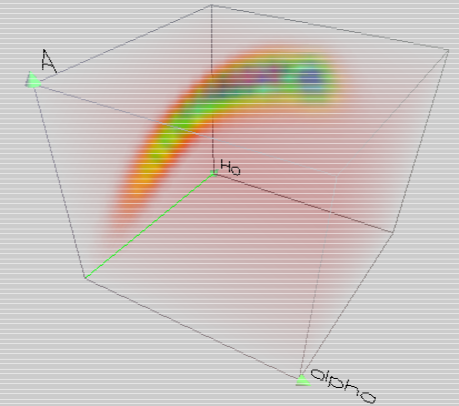
Figure 1: The graphics of the joint PDF as function of $(\alpha,H_{0},\bar{A})$ for the generalized Chaplygin gas model when fixing $k=0$ and $\Omega_{m0}=0.04$. It is a $3D$ density plot where the function (here the PDF) is rendered as semi-transparent colourful gas, or we can say that the plot is made by voxels (volume elements) analogous to pixels (picture elements). Where the PDF is minimum, the transparency is total and the colour is red, where the PDF is maximum then the voxel is opaque and the colour is violet; mid-range values are semi-transparent and coloured between red and violet (red, orange, yellow, green, blue, violet). The parameter ranges are $-1<\alpha\leqslant 9$, $62\leqslant H_{0}\leqslant 68$ and $0.5\leqslant\bar{A}\leqslant 1$, with resolutions $0.25\times 0.5\times 0.01$, respectively. The joint PDF of $(\alpha,H_{0},\bar{A})$ for other cases ($5$ free parameters, $4$ free parameters, etc.) show a similar $3D$ shape.

	GCGM	GCGM :	GCGM :	GCGM :	GCGM : $k=0$,	GCGM : $k=0$,
		$k=0$	$\Omega_{m0}=0$	$\Omega_{m0}=0.04$	$\Omega_{m0}=0$	$\Omega_{m0}=0.04$
$\alpha$	$-0.75_{-0.24}^{+4.04}$	$1.18_{-2.18}^{+4.12}$	$-0.05_{-0.79}^{+5.36}$	$-0.10_{-0.76}^{+5.10}$	$1.57_{-1.97}^{+4.86}$	$1.52_{-1.97}^{+4.53}$
$H_{0}$	$65.00_{-1.75}^{+1.77}$	$64.51_{-1.56}^{+1.64}$	$64.92_{-1.82}^{+1.80}$	$64.91_{-1.81}^{+1.80}$	$64.92_{-1.65}^{+1.55}$	$64.82_{-1.61}^{+1.54}$
$\Omega_{k0}$	$-0.77_{-5.94}^{+1.14}$	$0$	$0.00_{-2.94}^{+0.66}$	$0.06_{-3.03}^{+0.66}$	$0$	$0$
$\Omega_{m0}$	$0.00_{-0.00}^{+1.95}$	$0.00_{-0.00}^{+0.30}$	$0$	$0.04$	$0$	$0.04$
$\Omega_{c0}$	$1.36_{-0.85}^{+5.36}$	$1.00_{-0.30}^{+0.0}$	$1.00_{-0.66}^{+2.94}$	$1.02_{-0.66}^{+3.03}$	$1$	$0.96$
$\bar{A}$	$1.000_{-0.534}^{+0.000}$	$0.989_{-0.245}^{+0.011}$	$0.988_{-0.488}^{+0.012}$	$0.988_{-0.522}^{+0.012}$	$0.987_{-0.293}^{+0.013}$	$0.987_{-0.277}^{+0.012}$
$t_{0}$	$12.63_{-1.19}^{+2.04}$	$13.70_{-0.88}^{+1.82}$	$13.28_{-1.46}^{+2.31}$	$13.16_{-1.40}^{+2.48}$	$13.40_{-0.73}^{+1.18}$	$13.54_{-0.64}^{+1.48}$
$q_{0}$	$-0.818_{-0.459}^{+0.381}$	$-0.711_{-0.247}^{+0.298}$	$-0.787_{-0.446}^{+0.431}$	$-0.828_{-0.480}^{+0.461}$	$-0.878_{-0.062}^{+0.388}$	$-0.881_{-0.059}^{+0.370}$
$a_{i}$	$0.746_{-0.115}^{+0.057}$	$0.721_{-0.176}^{+0.121}$	$0.762_{-0.171}^{+0.087}$	$0.765_{-0.195}^{+0.102}$	$0.770_{-0.132}^{+0.065}$	$0.757_{-0.152}^{+0.066}$
$p(\alpha>0)$	$41.98\,\%$	$87.65\,\%$	$81.59\,\%$	$79.34\,\%$	$96.40\,\%$	$95.52\,\%$
$p(\alpha=1)$	$19.58\,\%$	$91.09\,\%$	$59.93\,\%$	$55.78\,\%$	$69.98\,\%$	$72.70\,\%$
$p(\Omega_{k0}<0)$	$96.29\,\%$	$-$	$70.35\,\%$	$75.19\,\%$	$-$	$-$
$p(\Omega_{k0}=0)$	$37.04\,\%$	$-$	$3.35\,\sigma$	$90.80\,\%$	$-$	$-$
$p(\bar{A}\neq 1)$	$0.00\,\%$	$59.15\,\%$	$99.96\,\%$	$98.57\,\%$	$100\,\%$	$100\,\%$
$p(q_{0}<0)$	$6.61\,\sigma$	$6.99\,\sigma$	$100\,\%$	$100\,\%$	$100\,\%$	$100\,\%$
$p(a_{i}<1)$	$6.88\,\sigma$	$7.49\,\sigma$	$100\,\%$	$100\,\%$	$100\,\%$	$100\,\%$

Table 4: The estimated parameters for the generalized Chaplygin gas model (GCGM) and some specific cases of spatial section and matter content. We use the Bayesian analysis to obtain the peak of the one-dimensional marginal probability and the $2\,\sigma$ credible region for each parameter. $H_{0}$ is given in $km/M\!pc.s$, $\bar{A}$ in units of $c$, $t_{0}$ in $Gy$ and $a_{i}$ in units of $a_{0}$.

	CGM	CGM :	CGM :	CGM :	CGM : $k=0$,	CGM : $k=0$,
		$k=0$	$\Omega_{m0}=0$	$\Omega_{m0}=0.04$	$\Omega_{m0}=0$	$\Omega_{m0}=0.04$
$H_{0}$	$65.01_{-1.71}^{+1.81}$	$64.48_{-1.53}^{+1.53}$	$64.93_{-1.77}^{+1.81}$	$64.93_{-1.76}^{+1.80}$	$64.67_{-1.52}^{+1.53}$	$64.64_{-1.51}^{+1.52}$
$\Omega_{k0}$	$-2.73_{-0.97}^{+1.53}$	$0$	$-0.22_{-1.10}^{+0.77}$	$-0.24_{-1.09}^{+0.73}$	$0$	$0$
$\Omega_{m0}$	$0.00_{-0.00}^{+1.22}$	$0.00_{-0.00}^{+0.29}$	$0$	$0.04$	$0$	$0.04$
$\Omega_{c0}$	$1.34_{-0.70}^{+0.94}$	$1.00_{-0.29}^{+0.00}$	$1.22_{-0.77}^{+1.10}$	$1.20_{-0.73}^{+1.09}$	$1$	$0.96$
$\bar{A}$	$1.000_{-0.270}^{+0.000}$	$0.857_{-0.072}^{+0.141}$	$0.746_{-0.080}^{+0.165}$	$0.759_{-0.083}^{+0.166}$	$0.812_{-0.071}^{+0.056}$	$0.834_{-0.072}^{+0.056}$
$t_{0}$	$12.73_{-1.14}^{+1.81}$	$14.07_{-0.62}^{+0.77}$	$13.20_{-1.31}^{+2.16}$	$13.20_{-1.31}^{+1.99}$	$14.02_{-0.59}^{+0.64}$	$14.01_{-0.57}^{+0.68}$
$q_{0}$	$-0.883_{-0.429}^{+0.382}$	$-0.654_{-0.113}^{+0.158}$	$-0.839_{-0.454}^{+0.417}$	$-0.860_{-0.428}^{+0.420}$	$-0.715_{-0.085}^{+0.109}$	$-0.700_{-0.082}^{+0.104}$
$a_{i}$	$0.739_{-0.088}^{+0.068}$	$0.698_{-0.075}^{+0.056}$	$0.754_{-0.136}^{+0.081}$	$0.724_{-0.111}^{+0.090}$	$0.705_{-0.050}^{+0.045}$	$0.709_{-0.53}^{+0.33}$
$p(\Omega_{k0}<0)$	$3.59\,\sigma$	$-$	$74.27\,\%$	$77.38\,\%$	$-$	$-$
$p(\Omega_{k0}=0)$	$0.04\,\%$	$-$	$64.54\,\%$	$59.18\,\%$	$-$	$-$
$p(\bar{A}\neq 1)$	$0.00\,\%$	$96.02\,\%$	$3.33\,\sigma$	$3.23\,\sigma$	$100\,\%$	$100\,\%$
$p(q_{0}<0)$	$7.59\,\sigma$	$100\,\%$	$100\,\%$	$100\,\%$	$100\,\%$	$100\,\%$
$p(a_{i}<1)$	$7.66\,\sigma$	$100\,\%$	$100\,\%$	$100\,\%$	$100\,\%$	$100\,\%$

Table 5: The estimated parameters for the traditional Chaplygin gas model (CGM) and some specific cases of spatial section and matter content. We use the Bayesian analysis to obtain the peak of the one-dimensional marginal probability and the $2\,\sigma$ credible region for each parameter. $H_{0}$ is given in $km/M\!pc.s$, $\bar{A}$ in units of $c$, $t_{0}$ in $Gy$ and $a_{i}$ in units of $a_{0}$.

	$\Lambda$CDM	$\Lambda$CDM :	$\Lambda$CDM :	$\Lambda$CDM :
		$k=0$	$\Omega_{m0}=0$	$\Omega_{m0}=0.04$
$H_{0}$	$65.00_{-1.74}^{+1.78}$	$64.29_{-1.51}^{+1.53}$	$64.02_{-1.53}^{+1.55}$	$64.07_{-1.54}^{+1.56}$
$\Omega_{k0}$	$-2.12_{-1.61}^{+1.96}$	$0$	$0.599_{-0.137}^{+0.155}$	$0.519_{-0.138}^{+0.155}$
$\Omega_{m0}$	$1.01_{-0.85}^{+1.08}$	$0.309_{-0.072}^{+0.082}$	$0$	$0.04$
$\Omega_{c0}$	$1.36_{-0.78}^{+0.92}$	$0.691_{-0.082}^{+0.072}$	$0.401_{-0.155}^{+0.137}$	$0.441_{-0.155}^{+0.138}$
$t_{0}$	$12.70_{-1.22}^{+2.15}$	$14.90_{-0.88}^{+0.82}$	$18.35_{-1.04}^{+1.19}$	$17.15_{-0.82}^{+0.85}$
$q_{0}$	$-0.864_{-0.405}^{+0.400}$	$-0.540_{-0.101}^{+0.136}$	$-0.410_{-0.131}^{+0.164}$	$-0.444_{-0.116}^{+0.186}$
$a_{i}$	$0.732_{-0.114}^{+0.083}$	$0.610_{-0.074}^{+0.077}$	$0$	$0.357_{-0.042}^{+0.048}$
$p(\Omega_{k0}<0)$	$98.08\,\%$	$-$	$0\,\%$	$0\,\%$
$p(\Omega_{k0}=0)$	$2.91\,\%$	$-$	$0\,\%$	$0\,\%$
$p(q_{0}<0)$	$7.57\,\sigma$	$100\,\%$	$5.12\,\sigma$	$5.08\,\sigma$
$p(a_{i}<1)$	$7.58\,\sigma$	$100\,\%$	$5.12\,\sigma$	$5.17\,\sigma$

Table 6: The estimated parameters for the $\Lambda$CDM model and some specific cases of spatial section and matter content. We use the Bayesian analysis to obtain the peak of the one-dimensional marginal probability and the $2\,\sigma$ credible region for each parameter. $H_{0}$ is given in $km/M\!pc.s$, $t_{0}$ in $Gy$ and $a_{i}$ in units of $a_{0}$.

From the probability distribution (18), a joint probability distribution for any subset of parameters can be obtained by integrating (marginalizing) on the remaining parameters, see refs. [15, 16]. This is a valuable information. But, in order to estimate properly a single parameter, the probability distribution must be marginalized on all other parameters. This in general gives a quite different result if we try to estimate the parameter in a two or three-dimensional parameter space. The reason is that, in such multidimensional parameter space, if a parameter has a large probability density but in a narrow region, the total contribution of this region may be quite small compared to other large regions which have small probability: in the marginalization process, this kind of high PDF region contributes little to the estimation of a given parameter. These features are exemplified in figure 1 where the probability distribution function (PDF) for the set of parameters ($\alpha,H_{0},\bar{A}$) in the GCGM case is displayed, with a clearly non-Gaussian behaviour. Hence, in what follows the estimation of a given parameter will be made by marginalizing on all other ones.

3.1 Estimation of $\alpha$

In the case of five free parameters, the procedure described above gives $\alpha=-0.75_{-0.24}^{+4.04}$. Note that this prediction differs substantially from that extracted from the minimization of $\chi^{2}$, which gives a large positive best value $\alpha$, instead of a negative $\alpha$ when the marginalization is made. Concerning the best value when the marginalization is made, even if the best value is negative, the dispersion is quite high, so even large positive values are not excluded, at least at $2\sigma$ level. Comparing our results with other ones already published requires some care due to the fact that usually in the works already quoted some parameters are fixed. Moreover, the allowed values for $\alpha$ are generally restricted to the interval $[0,1]$, except in references [19, 27, 28, 29, 30]. In reference [19], the authors considered $-1\leq\alpha<1$, a flat spatial section and they have fixed the value of the Hubble constant. They found a best value around $\alpha\sim 0.4$.

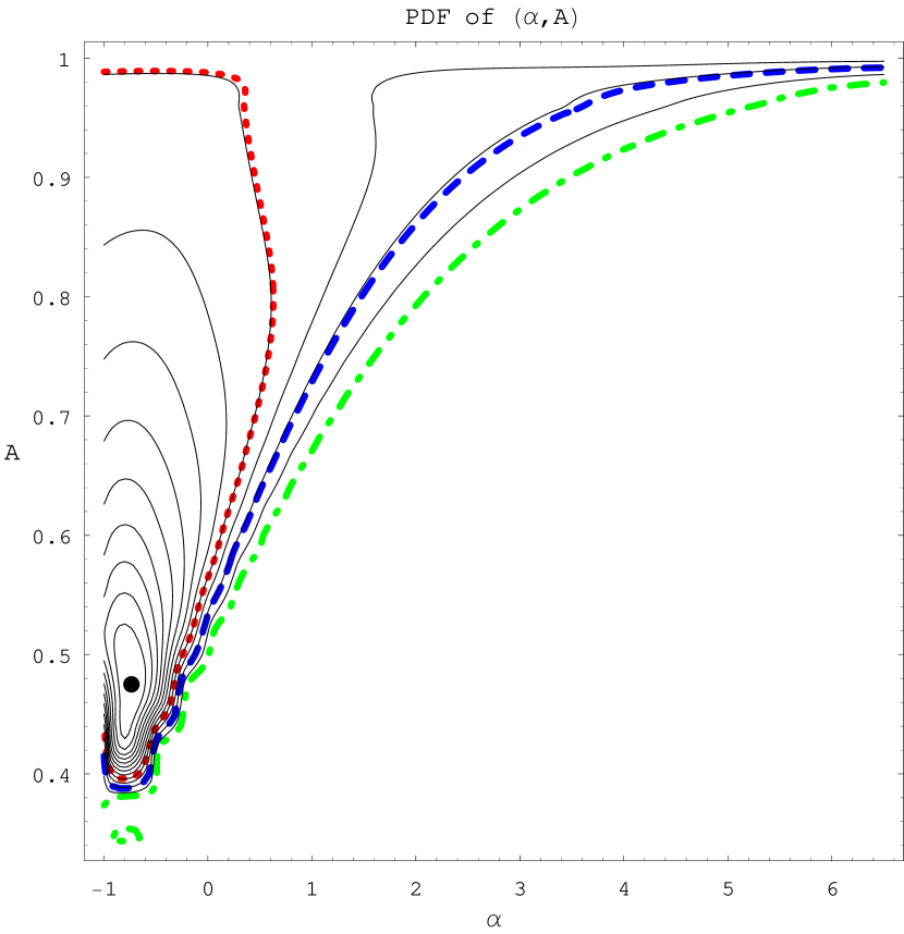
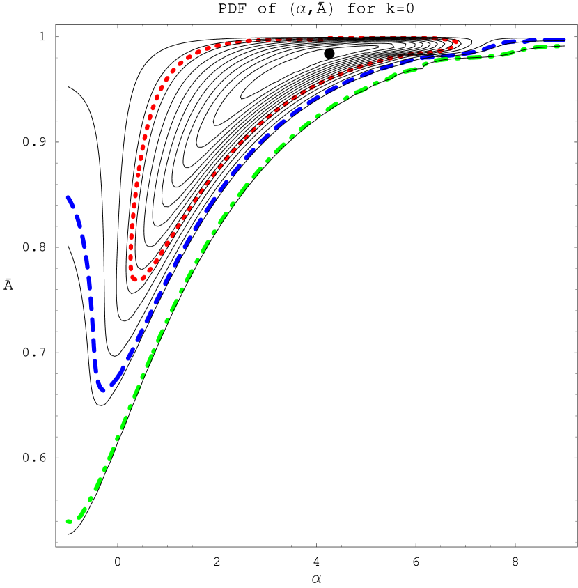
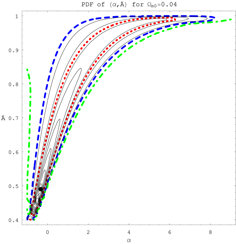
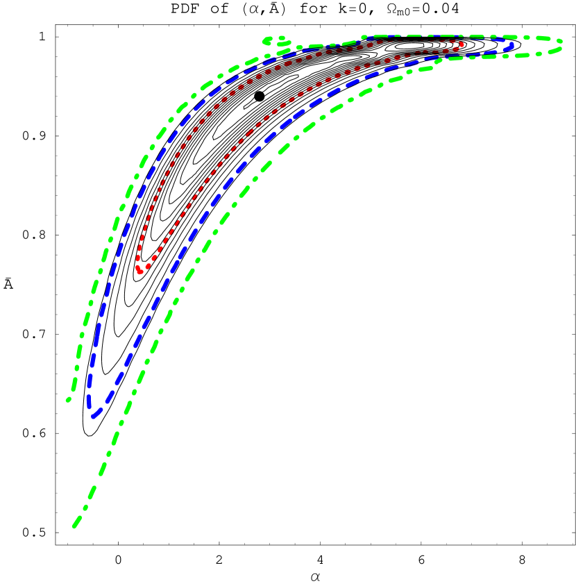
Figure 2: The graphics of the joint PDF as function of $(\alpha,\bar{A})$ for the generalized Chaplygin gas model. The joint PDF peak is shown by the large dot, the credible regions of $1\,\sigma$ ($68,27\%$) by the red dotted line, the $2\,\sigma$ ($95,45\%$) in blue dashed line and the $3\,\sigma$ ($99,73\%$) in green dashed-dotted line. The cases for $\Omega_{m0}=0$ are not shown here because they are similar to the ones with $\Omega_{m0}=0.04$.

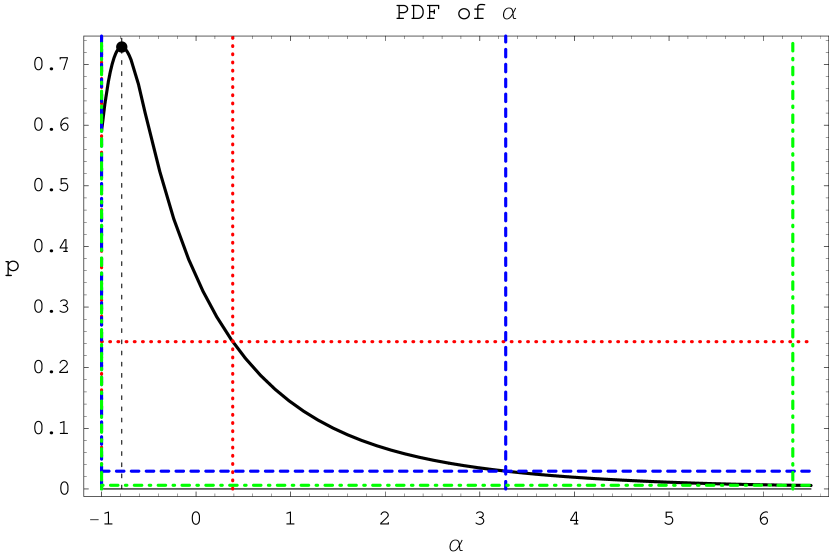
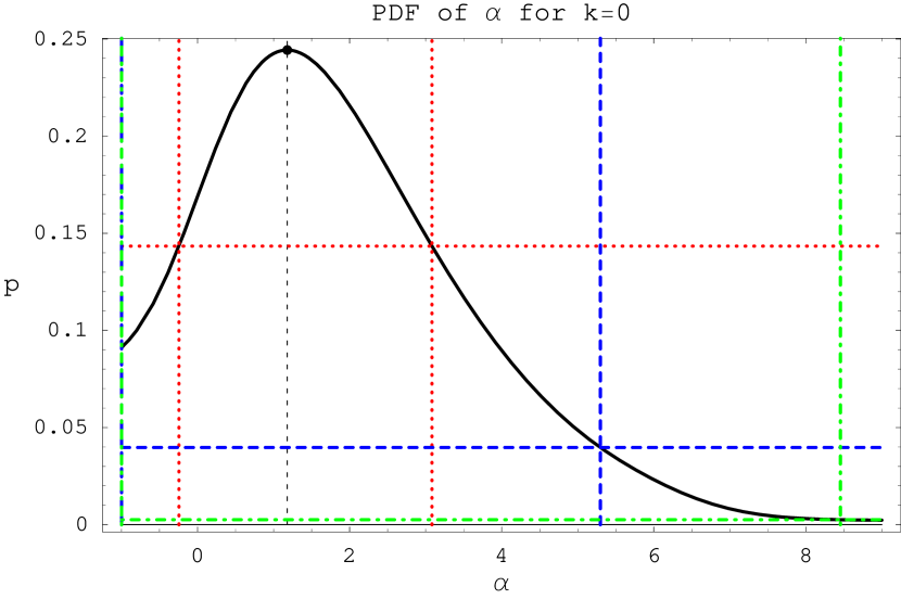
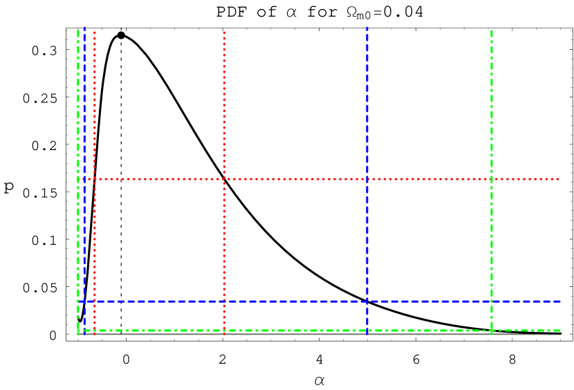
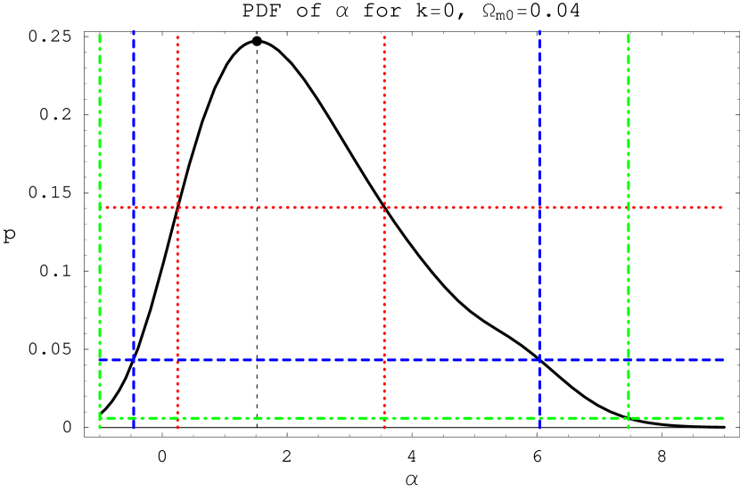
Figure 3: The PDF of $\alpha$ for the generalized Chaplygin gas model. The solid lines are the PDF, the $1\sigma$ ($68.27\%$) regions are delimited by red dotted lines and the $2\sigma$ ($95.45\%$) credible regions are given by blue dashed lines. The cases for $\Omega_{m0}=0$ are not shown here because they are similar to the ones with $\Omega_{m0}=0.04$.

If we compare with the results of ref. [16], the use of a large sample of supernovae has slightly diminished the best value, but at same time, it has reduced considerably the dispersion. Imposing that the space is flat, or fixing the pressureless matter equal to zero or $0.04$, lead to a positive best value for $\alpha$; the dispersion is also affected. For example, with the imposition that $k=0$ and $\Omega_{m}=0.04$, the estimation leads to $\alpha=1.52^{+4.53}_{-1.97}$. In figure 3 the PDF for $\alpha$ is displayed for the case of five parameters, and also for three particular cases, where one or two parameter is fixed. Note that as the baryonic matter or the curvature (or both) is fixed, the maximum of the PDF is displaced to positive values. In general grounds, we can state that even relatively large values for $\alpha$ are not excluded. Of course, for the CGM the value of $\alpha$ is fixed to unity. However, from the analysis for the GCGM it can be inferred that the probability to have $\alpha=1$ is $19.58\%$ when the five parameters are free. Restricting to null curvature or fixing the pressureless density increases considerably this value: for example, when the curvature is null the probability to have $\alpha=1$ is about $90\%$. At the same time, the probability to have $\alpha>1$ is $41.98\%$ when all parameters are free, but this value can double when one or two parameters are fixed.

3.2 Estimation of $\bar{A}$

In general the results indicate that the value of $\bar{A}$ is close to unity. When five free parameters are considered, the marginalization of the remaining four other parameters leads to $\bar{A}=1.000_{-0.534}^{+0.000}$. This may suggest the conclusion that $\Lambda$CDM ($\bar{A}=1$) model is favoured. However, the accuracy of the computation, due to the step (between $0.01$ and $0.02$) used in the evaluation of the parameter, does not allow this conclusion. Instead, it means the peak happens for $0.98<\bar{A}\leqslant 1$.

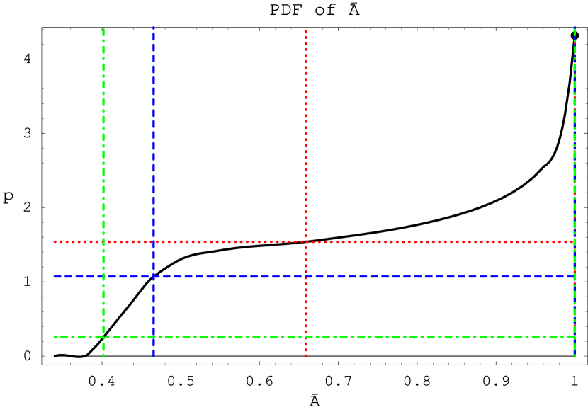
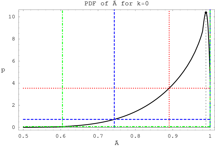
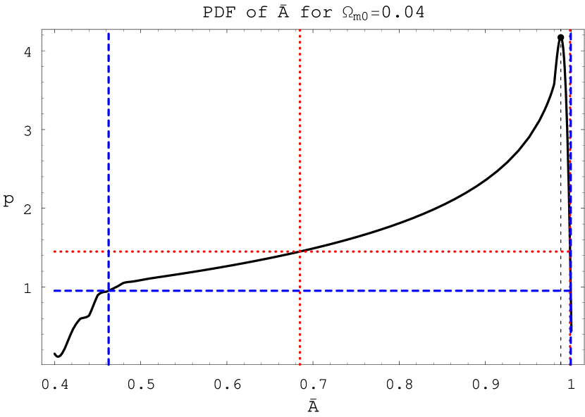
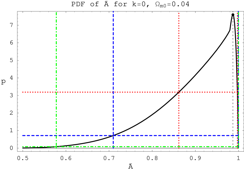
Figure 4: The one-dimensional PDF of $\bar{A}$ for the generalized Chaplygin gas model. The solid lines are the PDF, the $1\sigma$ ($68.27\%$) regions are delimited by red dotted lines, the $2\sigma$ ($95.45\%$) credible regions are given by blue dashed lines and the $3\sigma$ ($99.73\%$) regions are delimited by green dashed-dotted lines. The cases for $\Omega_{m0}=0$ are not shown here because they are similar to the ones with $\Omega_{m0}=0.04$.

In fact, fixing the curvature or the pressureless matter, the preferred value differs slightly from unity: with $\Omega_{m}=0.04$ and $k=0$, for example, we have $\bar{A}=0.987_{-0.272}^{+0.012}$. The situation is essentially the same for the CGM: when all other parameters are marginalized, the best value is unity, but with a small dispersion, $\bar{A}=1.000_{-0.270}^{+0.000}$; however, this best value becomes smaller when one or two parameters are fixed. This occurs in both for the GCGM and CGM. In figures 4 and 5 the PDF for $\bar{A}$ is displayed, both for the GCGM and the CGM, in the case where the marginalization is made in all other parameters, and when the matter density and/or the curvature is fixed. Fixing one or two parameters displaces the maximum of probability in the direction of smaller value of $\bar{A}$. This effect is more sensible for the CGM: in general, the best value of the CGM is smaller than in the GCGM, and the dispersion is also smaller. Note that the probability to have $\bar{A}\neq 1$ is zero when all parameters are free, both for the GCGM and CGM. But, this probability can become as high as $100\%$ when one or two parameters are fixed.

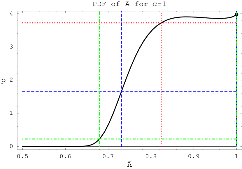
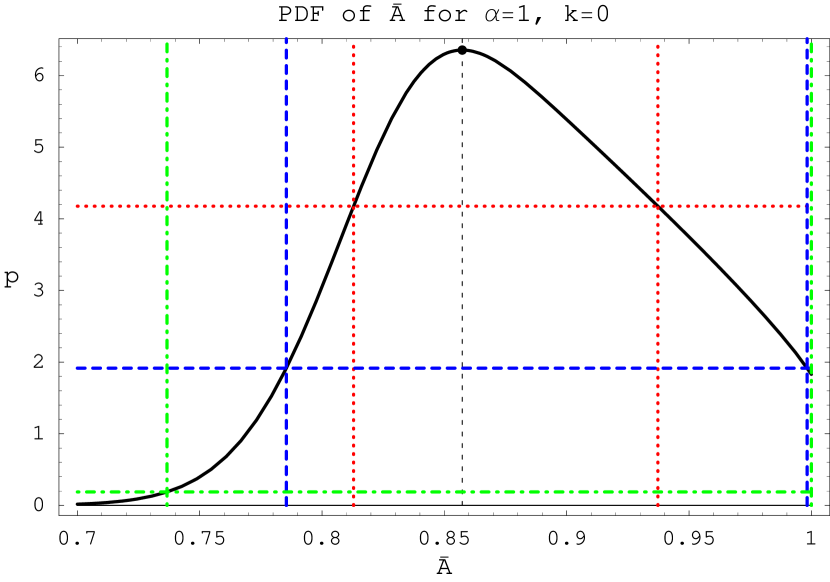
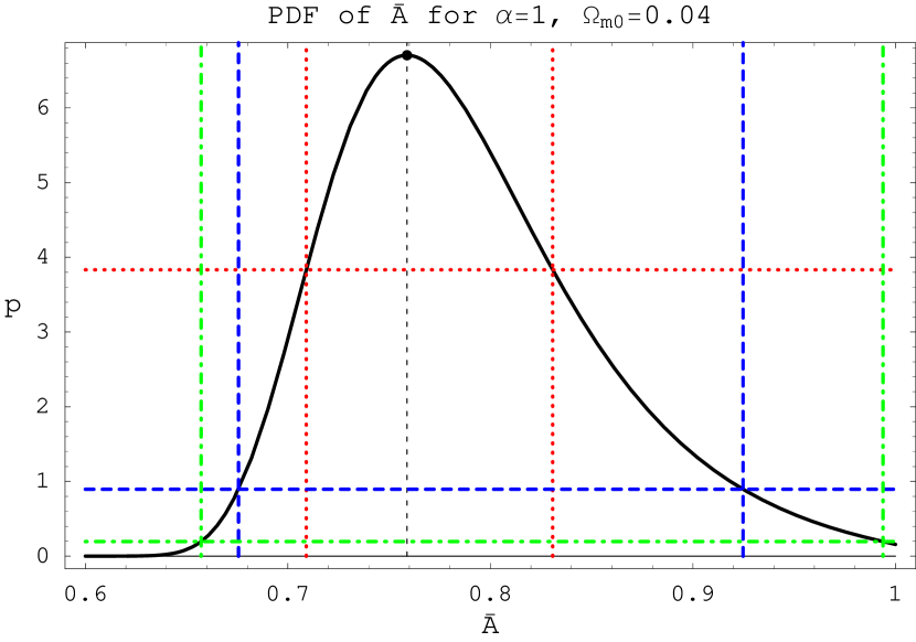
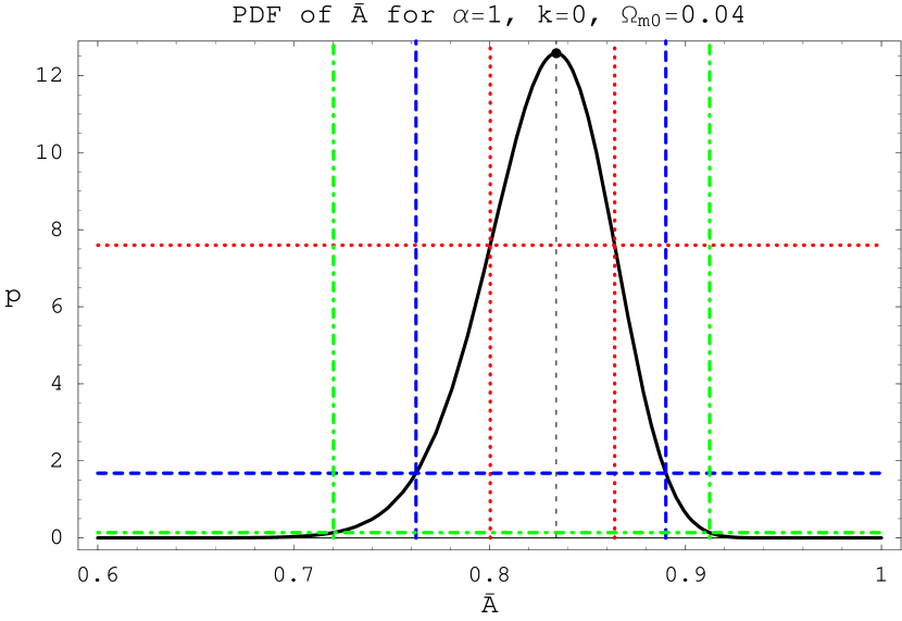
Figure 5: The one-dimensional PDF of $\bar{A}$ for the traditional Chaplygin gas model (CGM). The solid lines are the PDF, the $1\sigma$ ($68.27\%$) regions are delimited by red dotted lines, the $2\sigma$ ($95.45\%$) credible regions are given by blue dashed lines and the $3\sigma$ ($99.73\%$) regions are delimited by green dashed-dotted lines. The cases for $\Omega_{m0}=0$ are not shown here because they are similar to the ones with $\Omega_{m0}=0.04$.

In figure 2 the joint probabilities for $\alpha$ and $\bar{A}$ are displayed, with a non-Gaussian shape. This figure is an illustration of the importance of the marginalization process because it changes the peak values and credible regions depending if two or one-dimensional parameter space is used. The region of highest probability, at $2\sigma$ level, is concentrated around $\alpha=0$ with a large dispersion for $\bar{A}$, as the curvature and/or the pressureless matter is fixed, this region displaces itself to positive values of $\alpha$ and to higher values of $\bar{A}$, the opposite that happens with the PDF value of $\bar{A}$, due in the last case to the marginalization procedure. The dispersion in $\bar{A}$ remains always large. It is obvious, on the other hand, from the two-dimensional credible regions that the case $\alpha=1$ is not ruled out. Using a larger sample of $253$ data, the authors of reference [28] have constrained the parameters $\alpha$ and $\bar{A}$ such that $[1.6,3.6]$ and $[0.856,0.946]$ at $68\%$ confidence level. But they have used the $\chi^{2}$ statistics and quartessence, and in this sense their result may be considered as compatible with ours. In reference [14], restricting to the flat case, and fixing $\alpha=1$, for example, the authors have found that $0.66<\bar{A}<1$ at $95\%$ confidence level. This result is compatible with ours, see table $5$.

3.3 Estimation of $\Omega_{m0}$

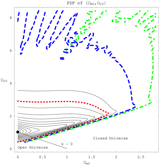
Figure 6: The graphics of the joint PDF as function of $(\Omega_{m0},\Omega_{c0})$ for the generalized Chaplygin gas model, where $p(\Omega_{m0},\Omega_{c0})$ is a integral of $p(\alpha,H_{0},\Omega_{m0},\Omega_{c0},\bar{A})$ over the $(\alpha,H_{0},\bar{A})$ parameter space. It shows a different shape for the confidence regions with respect to the $\Lambda CDM$ but similar to the CGM of ref. [16]. The joint PDF peak has the value $0.584$ for $(\Omega_{m0},\Omega_{c0})=(0.00,1.00)$ (shown by the large dot), the credible regions of $1\,\sigma$ ($68,27\%$, shown in red dotted line), $2\,\sigma$ ($95,45\%$, in blue dashed line) and $3\,\sigma$ ($99,73\%$, in green dashed-dotted line) have PDF levels of $0.104$, $0.037$ and $0.010$, respectively. As $\Omega_{k0}+\Omega_{m0}+\Omega_{c0}=1$, the probability for a spatially flat Universe is on the line $\Omega_{m0}+\Omega_{c0}=1$, above it we have the region for a closed Universe ($k>0$, $\Omega_{k0}<0$), and below, the region for an open Universe ($k<0$, $\Omega_{k0}>0$).

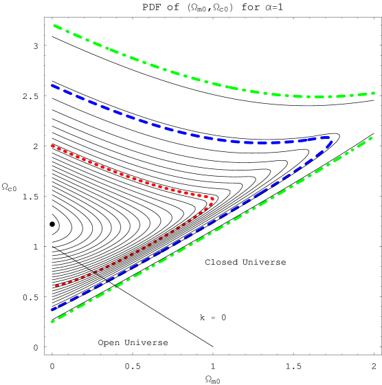
Figure 7: The graphics of the joint PDF as function of $(\Omega_{m0},\Omega_{c0})$ for the traditional Chaplygin gas model (CGM), where $p(\Omega_{m0},\Omega_{c0})$ is a integral of $p(H_{0},\Omega_{m0},\Omega_{c0},\bar{A})$ over the $(H_{0},\bar{A})$ parameter space. It shows a different shape for the confidence regions with respect to the $\Lambda CDM$ but similar to the CGM of ref. [16]. The joint PDF peak has the value $1.473$ for $(\Omega_{m0},\Omega_{c0})=(0.00,1.22)$ (shown by the large dot), the credible regions of $1\,\sigma$ ($68,27\%$, shown in red dotted line), $2\,\sigma$ ($95,45\%$, in blue dashed line) and $3\,\sigma$ ($99,73\%$, in green dashed-dotted line) have PDF levels of $0.542$, $0.103$ and $0.009$, respectively. As $\Omega_{k0}+\Omega_{m0}+\Omega_{c0}=1$, the probability for a spatially flat Universe is on the line $\Omega_{m0}+\Omega_{c0}=1$, above it we have the region for a closed Universe ($k>0$, $\Omega_{k0}<0$), and below, the region for an open Universe ($k<0$, $\Omega_{k0}>0$).

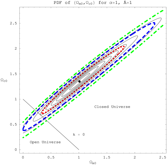
Figure 8: The graphics of the joint PDF as function of $(\Omega_{m0},\Omega_{c0})$ for the $\Lambda$CDM model model, where $p(\Omega_{m0},\Omega_{c0})$ is a integral of $p(H_{0},\Omega_{m0},\Omega_{c0})$ over the $H_{0}$ parameter space. The joint PDF peak has the value $4.22$ for $(\Omega_{m0},\Omega_{c0})=(1.01,1.35)$ (shown by the large dot), the credible regions of $1\,\sigma$ ($68,27\%$, shown in red dotted line), $2\,\sigma$ ($95,45\%$, in blue dashed line) and $3\,\sigma$ ($99,73\%$, in green dashed-dotted line) have PDF levels of $1.380$, $0.247$ and $0.025$, respectively. As $\Omega_{k0}+\Omega_{m0}+\Omega_{c0}=1$, the probability for a spatially flat Universe is on the line $\Omega_{m0}+\Omega_{c0}=1$, above it we have the region for a closed Universe ($k>0$, $\Omega_{k0}<0$), and below, the region for an open Universe ($k<0$, $\Omega_{k0}>0$).

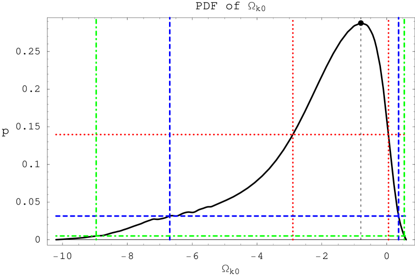
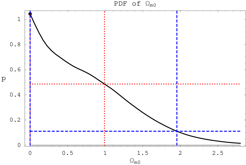
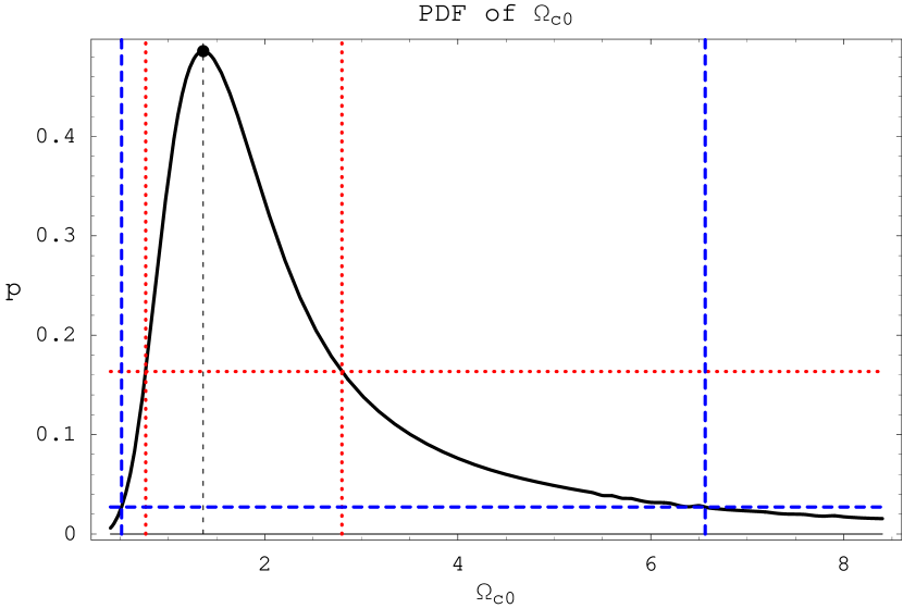
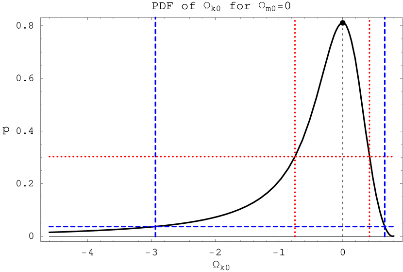
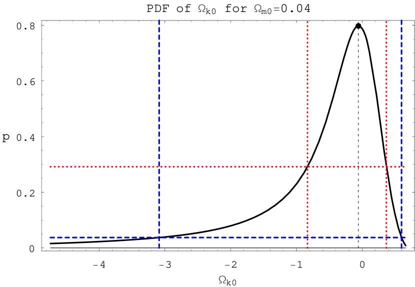
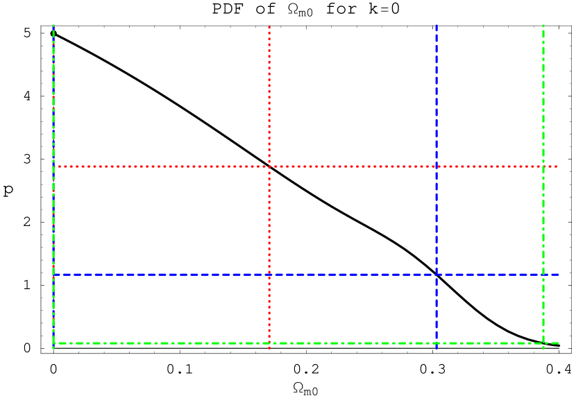
Figure 9: The one-dimensional PDF of $\Omega_{k0}$, $\Omega_{m0}$ and $\Omega_{c0}$ for the generalized Chaplygin gas model. The solid lines are the PDF, the $1\sigma$ ($68.27\%$) regions are delimited by red dotted lines, the $2\sigma$ ($95.45\%$) credible regions are given by blue dashed lines and the $3\sigma$ ($99.73\%$) regions are delimited by green dashed-dotted lines. As $\Omega_{c0}=1-\Omega_{k0}-\Omega_{k0}$, for $\Omega_{m0}=0$ we have $\Omega_{c0}=1-\Omega_{k0}$, for $\Omega_{m0}=0.04$ then $\Omega_{c0}=0.96-\Omega_{k0}$ and for $\Omega_{k0}=0$ we also have $\Omega_{c0}=1-\Omega_{m0}$.

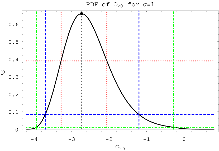
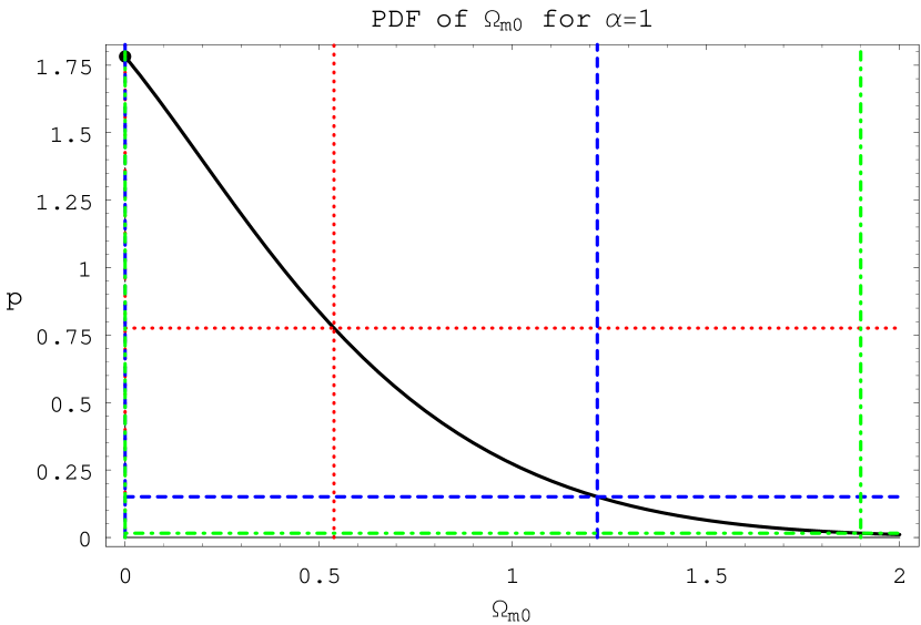
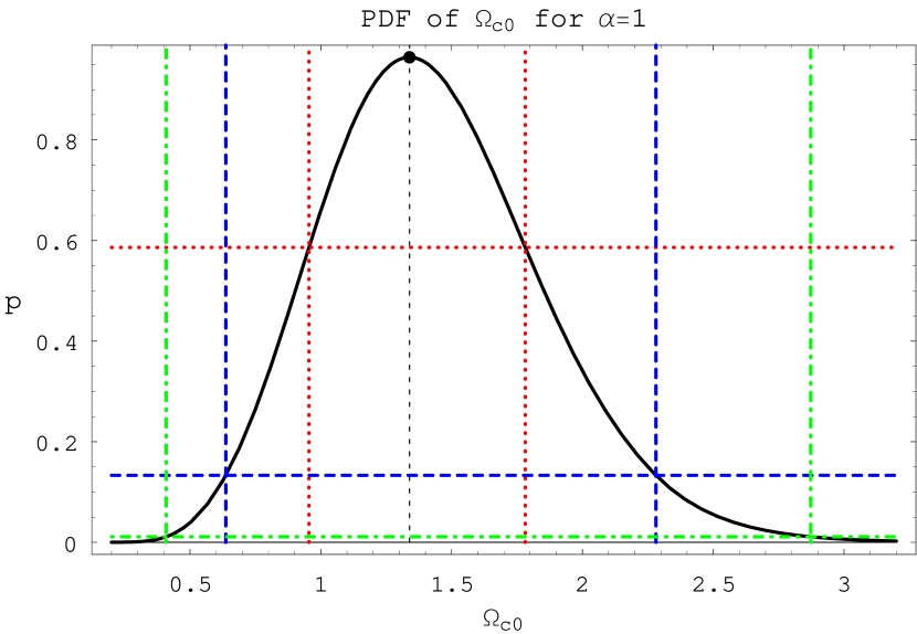
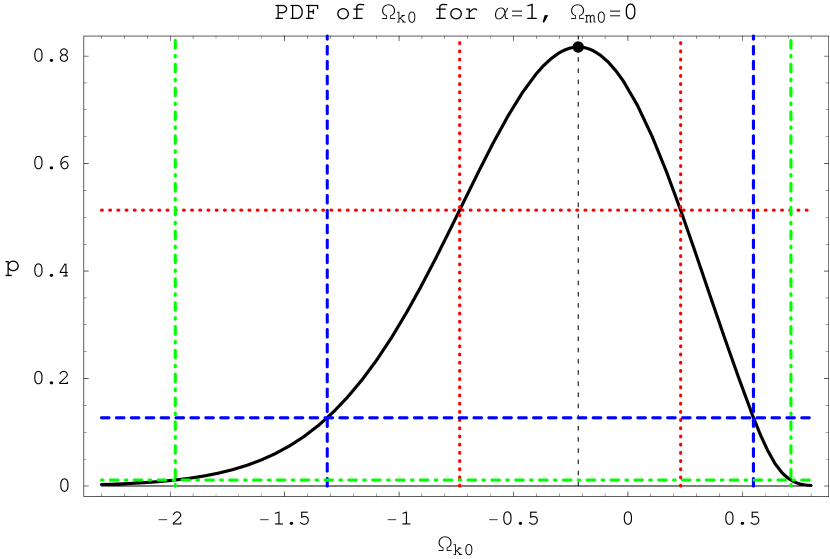
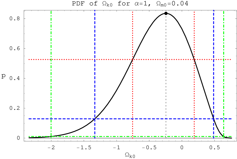
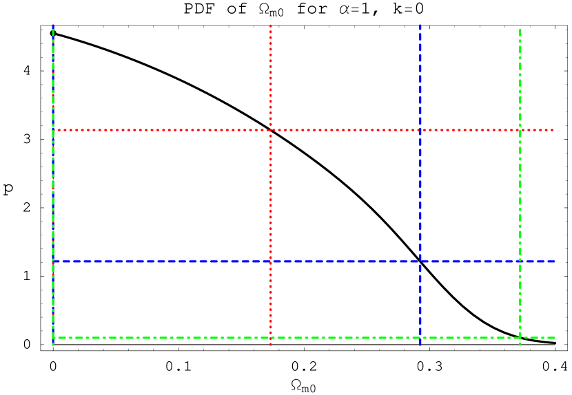
Figure 10: The one-dimensional PDF of $\Omega_{k0}$, $\Omega_{m0}$ and $\Omega_{c0}$ for the traditional Chaplygin gas model. The solid lines are the PDF, the $1\sigma$ ($68.27\%$) regions are delimited by red dotted lines, the $2\sigma$ ($95.45\%$) credible regions are given by blue dashed lines and the $3\sigma$ ($99.73\%$) regions are delimited by green dashed-dotted lines. As $\Omega_{c0}=1-\Omega_{k0}-\Omega_{k0}$, for $\Omega_{m0}=0$ we have $\Omega_{c0}=1-\Omega_{k0}$, for $\Omega_{m0}=0.04$ then $\Omega_{c0}=0.96-\Omega_{k0}$ and for $\Omega_{k0}=0$ we also have $\Omega_{c0}=1-\Omega_{m0}$.

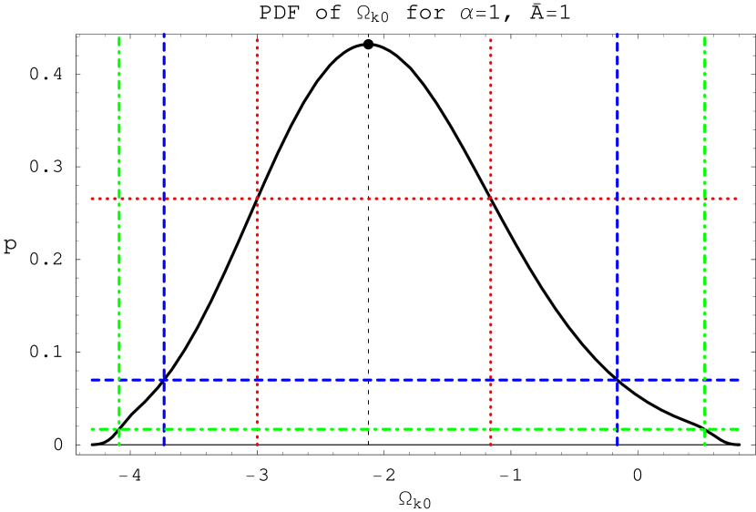
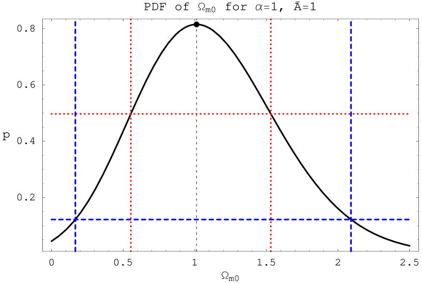
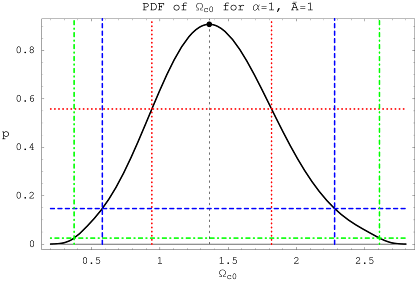
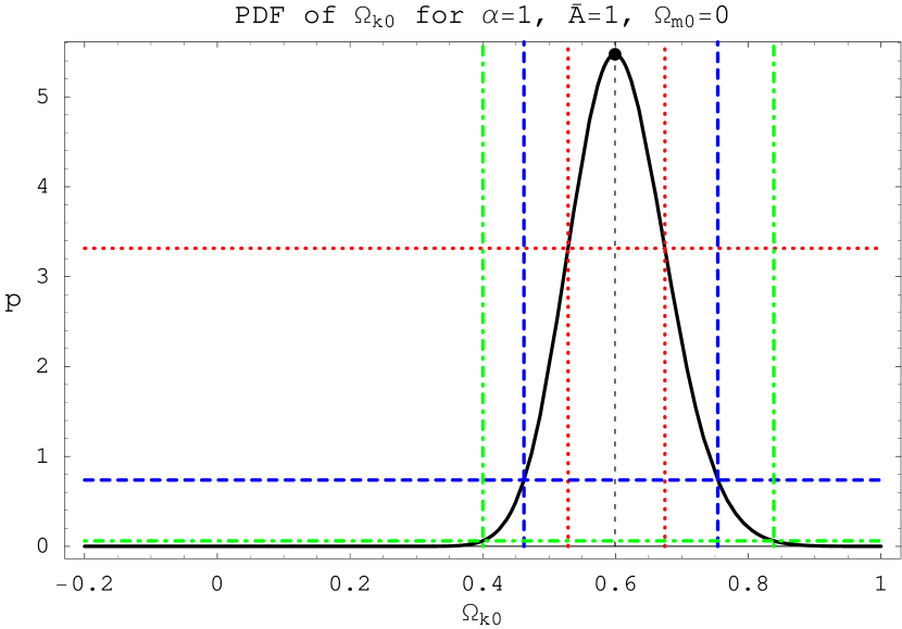
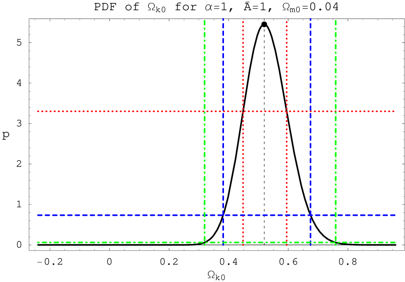
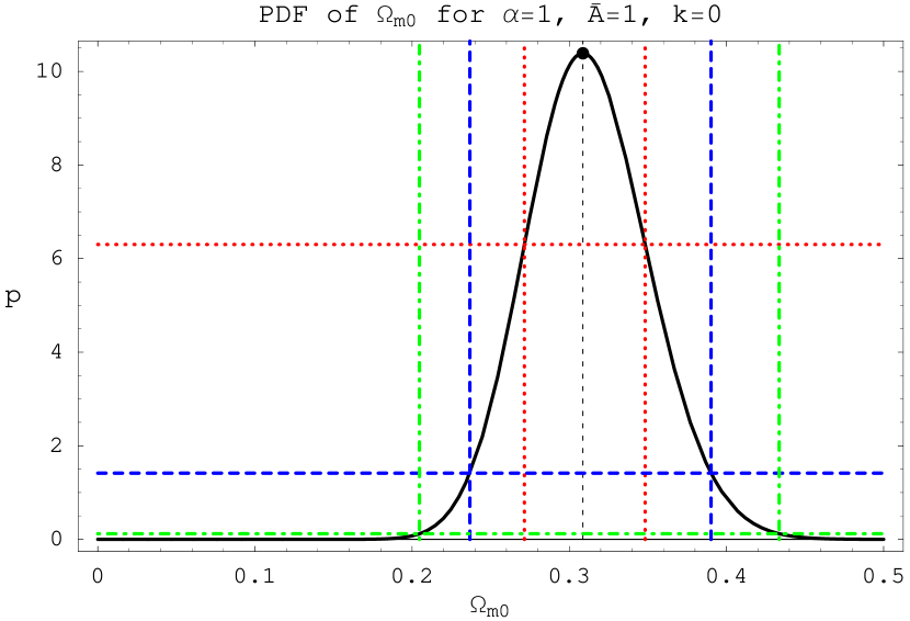
Figure 11: The one-dimensional PDF of $\Omega_{k0}$, $\Omega_{m0}$ and $\Omega_{c0}$ for the $\Lambda$CDM model. The solid lines are the PDF, the $1\sigma$ ($68.27\%$) regions are delimited by red dotted lines, the $2\sigma$ ($95.45\%$) credible regions are given by blue dashed lines and the $3\sigma$ ($99.73\%$) regions are delimited by green dashed-dotted lines. As $\Omega_{c0}=1-\Omega_{k0}-\Omega_{k0}$, for $\Omega_{m0}=0$ we have $\Omega_{c0}=1-\Omega_{k0}$, for $\Omega_{m0}=0.04$ then $\Omega_{c0}=0.96-\Omega_{k0}$ and for $\Omega_{k0}=0$ we also have $\Omega_{c0}=1-\Omega_{m0}$.

The most general case where all five parameters are free in the GCGM predict $\Omega_{m0}=0.00^{+1.95}_{-0.00}$, while for the CGM, $\Omega_{m0}=0.00^{+1.22}_{-0.00}$. Hence, the unified scenario, with no pressureless matter, is favoured, but the dispersion is very high. Among the particular situations, where some of the parameters are fixed, the only relevant case is the flat Universe, which favours still the unified model, but with a much smaller dispersion. Repeating the analysis for $\Lambda$CDM, we find $\Omega_{m0}=1.01^{+1.08}_{-0.85}$. This prediction is a very important distinctive feature of $\Lambda$CDM with respect to the GCGM. In reference [18], using a large sample of supernovae, the estimated value for the pressureless matter component, for $\Lambda$CDM, was $\Omega_{m0}=0.28\pm 0.05$ for a flat Universe. A similar value has been obtained in reference [17], who employed also a very large sample of supernovae: $0.29^{+0.05}_{-0.03}$. In this case, our analysis gives $\Omega_{m0}=0.309^{+0.082}_{-0.072}$, with a good agreement. The analysis of the WMAP data leads to $\Omega_{m0}=0.14\pm 0.02$ [4]. All these results are in some sense compatible due to the large error bar in our estimation.

3.4 Estimation of $\Omega_{c0}$

Remarkably, the GCGM, the CGM and the $\Lambda$CDM leads to almost the same predictions concerning the dark energy component when all parameters are free: $1.36^{+5.36}_{-0.85}$, $1.34^{+0.94}_{-0.70}$ and $1.36^{+0.92}_{-0.78}$, respectively. The best value does change appreciably when one or two parameters are fixed. The most important distinguishing feature is the dispersion, that is considerably higher, mainly in the upper uncertainty, for the GCGM. In comparison with the studies performed with a restricted sample of supernovae [15, 16], the main modification is the narrowing of the dispersion. The joint probability for $\Omega_{c0}$ and $\Omega_{m0}$ reflects what has been said in this and in the preceding sub-section. For the $\Lambda$CDM case, the two-dimensional picture for $\Omega_{c0}$ and $\Omega_{m0}$ display an ellipse, with the best value around ($1,1$), while the ellipse is highly distorted for the $GCGM$ and $CGM$ cases, with the best value around ($1,0$). Moreover, the $1\sigma$, $2\sigma$ and $3\sigma$ contours are expressively displaced to the top of the diagram, mainly for the GCGM, what is a consequence of the high dispersion in this case.

3.5 Estimation of $\Omega_{k0}$

Both in the GCGM and in the CGM, a closed Universe is clearly favoured: $\Omega_{k0}=-0.77^{+1.14}_{-5.94}$ and $\Omega_{k0}=-2.73^{+1.53}_{-0.97}$, respectively. The dispersion, however is quite large. The quantity of pressureless matter displaces the maximum of probability to a value near or equal to zero and narrows the dispersion. Curiously, the dispersion for the GCGM has increased in comparison with the restricted sample of supernovae used in reference [16], while for the CGM it has remained almost the same. A similar behaviour occurs in the dispersion of the other mass density parameters. For the GCGM the probability to have a closed Universe is $96.29\%$; when the pressureless matter is fixed equal zero or equal to the baryonic content, this probability is smaller, $69.43\%$ and $74.40\%$, respectively. The probability to have a flat Universe is $37.04\%$. For the CGM, such numbers increase slightly : for example, the probability to have a closed Universe is extremely near $100\%$: $3.59\sigma$. In this case, the probability to have a flat Universe is only $0.04\%$, but increases to near $60\%$ after setting the pressureless matter. The $\Lambda$CDM model favours also a closed Universe: $\Omega_{k0}=-2.12^{+1.96}_{-1.61}$, but an open Universe is favoured when the pressureless component is fixed. Moreover, the probability to have a closed Universe in the $\Lambda$CDM is $98.08\%$ when all free parameters are taken into account, but this value drops to zero when the curvature or the pressureless matter component is fixed. In principle the $\Lambda$CDM gives estimations closer to the CGM, but it must be remarked that the dispersion is very large.

3.6 Estimation of $H_{0}$

The predicted value of the Hubble constant today $H_{0}$ is the most robust one. This can be understood by looking at the expression for the luminosity distance: the Hubble constant appears as an overall multiplicative factor. The predictions are: $H_{0}=65.00^{+1.77}_{-1.75}$ for the GCGM and $H_{0}=65.01^{+1.81}_{-1.71}$ for the CGM. Fixing the curvature and/or the pressureless matter changes very slightly these predictions. Note that the dispersion is relatively small. In comparison with the restricted sample of references [15, 16] the best value for the Hubble constant has increased a little, and the dispersion has diminished. Repeating the analysis for the $\Lambda$DCM, we find $H_{0}=65.00^{+1.78}_{-1.74}$, very near the values found for the GCGM and CGM. The estimated value differs, on the other hand, from the predictions coming from CMBR, without a superposition of error bars: the WMAP predicts $H_{0}=72\pm 0.5$ [4].

3.7 Estimation of the age of the Universe, $t_{0}$

The predicted age of the Universe for the GCGM is $t_{0}=12.63^{+2.04}_{-1.19}\,Gy$ and for the CGM $t_{0}=12.73^{+1.81}_{-1.44}\,Gy$. These values are dangerously near the recent estimations age of the globular clusters [34], $t_{0}=12.6^{+3.4}_{-2.4}\,Gy$. However, the error bars remain quite large. The estimation of the age of the Universe using the WMAP data gives $13.4\pm 0.3\,Gy$ [4]. Compared with the previous analysis with a sub-sample of the supernovae, the predicted age has considerably diminished [15, 16]. Fixing the curvature and/or the pressureless matter increases slightly the predicted age (this is the opposite behaviour when sub-sample of 26 supernovae is used). Considering now the $\Lambda$CDM, the estimation of the age of the Universe leads to $t_{0}=12.70^{+2.15}_{-1.22}$, in good agreement with the predictions of the GCGM and CGM. In the $\Lambda$CDM, however, values as high as $17\,Gy$ can be found by, for example, fixing $\Omega_{m0}=0.04$. Note that, for the GCGM, the best value for the product $H_{0}t_{0}$ is $0.84$, which is essentially the same for the other cases, while in reference [18], for the $\Lambda$CDM model, $H_{0}t_{0}=0.96$.

3.8 Estimation of the deceleration parameter $q_{0}$

The value for the deceleration parameter $q_{0}$ in the GCGM with five free parameters is given by $q_{0}=-0.818^{+0.381}_{-0.459}$. The particular cases where the curvature and/or pressureless matter are fixed change very slightly this value. On the other hand, fixing $\alpha=1$, $q_{0}=-0.883^{+0.382}_{-0.429}$. These best values have not changed appreciably with respect to the restricted sample of $26$ supernovae. However, the dispersion is considerably smaller. Repeating the analysis for the $\Lambda$CDM, we find $q_{0}=-0.864^{+0.400}_{-0.405}$, barely differing from the previous models. In all cases, the probability to have a negative value for the deceleration parameter is equal to or very near $100\%$.

3.9 Estimation of the moment the Universe begins to accelerate

Another useful quantity is the redshift at which the Universe begins to accelerate, $z_{i}$. Due to computational reasons, it is more practical to evaluate the value of the scale factor at the moment the Universe begins to accelerate $a_{i}$, keeping in mind that the scale factor is normalized with its present value equal to unity. For the GCGM with five parameters, we find $a_{i}=0.746_{-0.115}^{+0.057}$. Imposing the curvature and/or the pressureless matter component does not change appreciably this result. For the CGM we find $a_{i}=0.739^{+0.068}_{-0.088}$. In reference [16], the same analysis has been made for the GCGM with the restricted sample of supernovae: the value of $a_{i}$ was smaller, but the dispersion was considerably higher. For the $\Lambda$CDM we have $a_{i}=0.732^{+0.083}_{-0.114}$. In all cases, the probability the Universe begins to accelerate before today is essentially $100\%$. All these results must be compared with that obtained in reference [17] which gives, translated in our notation, $a_{i}=0.68^{+0.07}_{-0.05}$.

4 Conclusions

The aim of the present work was to present the most general analysis of the GCGM and CGM in what concerns the comparison of theoretical predictions with the type Ia supernovae data, using the 157 data of the “gold sample”. All free parameters for each model were considered. In the case of the GCGM there are five free parameter: the Hubble constant $H_{0}$; the equation of state parameter $\alpha$; the “sound velocity” related parameter $\bar{A}$; the curvature density of the Universe $\Omega_{k0}$; the density parameter for the pressureless matter (alternatively, the Chaplygin gas) $\Omega_{m0}$(alternatively, $\Omega_{c0}$). For the CGM, the number of parameters reduce to four, since $\alpha=1$. We have considered also the $\Lambda$CDM, where the number of parameters reduce to three: $H_{0}$, $\Omega_{k0}$ and $\Omega_{m0}$ (alternatively, $\Omega_{c0}$).

A Bayesian statistical analysis was employed in order to obtain the predictions, with the error bars, for each parameter in each model. In doing so, the marginalization procedure was used so the one parameter estimations become more robust. This procedure consists in integrating in the remaining parameters in order to obtain a prediction for a given parameter. The results are the following. For the GCGM, we obtained: $\alpha=-0.75_{-0.24}^{+4.04}$, $H_{0}=65.00_{-1.75}^{+1.77}$, $\Omega_{k0}=-0.77_{-5.94}^{+1.14}$, $\Omega_{m0}=0.00_{-0.00}^{+1.95}$, $\Omega_{c0}=1.36_{-0.85}^{+5.36}$, $\bar{A}=1.000_{-0.534}^{+0.000}$. The results for the CGM are: $H_{0}=65.01_{-1.71}^{+1.81}$, $\Omega_{k0}=-2.73_{-0.97}^{+1.53}$, $\Omega_{m0}=0.00_{-0.00}^{+1.22}$, $\Omega_{c0}=1.34_{-0.70}^{+0.94}$, $\bar{A}=1.000_{-0.270}^{+0.000}$. For the $\Lambda$CDM, we found: $H_{0}=65.00_{-1.74}^{+1.78}$, $\Omega_{k0}=-2.12_{-1.61}^{+1.96}$, $\Omega_{m0}=1.01_{-0.85}^{+1.08}$, $\Omega_{c0}=1.36_{-0.78}^{+0.92}$. We have also evaluated the age of the Universe, the value of the decelerating parameter today and the moment the Universe begins to accelerated. The results for the GCGM, the CGM and the $\Lambda$CDM are, respectively: $t_{0}=12.63_{-1.19}^{+2.04}$, $12.73_{-1.14}^{+1.81}$, $12.70_{-1.22}^{+2.15}$; $q_{0}=-0.818_{-0.459}^{+0.381}$, $-0.883_{-0.429}^{+0.382}$, $-0.864_{-0.405}^{+0.400}$; $a_{i}=0.746_{-0.115}^{+0.057}$, $0.739_{-0.088}^{+0.068}$, $0.732_{-0.114}^{-0.083}$.

In the GCGM, the best value for $\alpha$ is negative but, due to the large dispersion, high positive values are also allowed. This may be compared with the results of references [28, 29, 30], were $\alpha$ takes high positive values. In reference [28], the apparent discrepancy is due to the quartessence choice and the statistical method employed : the authors used the $\chi^{2}$ statistics in order to obtain the confidence regions. Other crucial parameter is $\bar{A}$. Both for the GCGM and CGM, the best value is in principle $1$, but the finite resolution used in the numerical computation suggests that the peak value of $\bar{A}$ can be between $0.98$ (or $0.99$) and $1.00$. Futhermore, the particular cases of fixed curvature and matter densities shows a value near but small than $1$ as the best value of $\bar{A}$, such that the $\Lambda$CDM case ($\bar{A}=1$) is almost ruled out.

The results reported above indicate that, for the GCGM, CGM and $\Lambda$CDM, a closed Universe is favoured. For the GCGM and CGM the unified scenario (quartessence), where the pressureless matter density is essentially zero, is also favoured. In any case, a small fraction of pressureless matter must be introduced in order to take into account the baryons. However, the dispersions are quite large, decreasing significantly for the flat Universe case. It is curious that in the $\Lambda$CDM, the density parameter for pressureless matter is around unity. The predictions for the dark energy component are similar for the three models, but in the GCGM the dispersion is very expressive, allowing for very large values for the density parameter of the dark energy.

The analyses made predict a not very old Universe for all three cases. The best value is compatible, for example, with the estimated age of the globular clusters [34]. However, it must be stressed that such compatibility is verified mainly because of the high dispersion in those evaluations. The predictions for the deceleration parameter and for the moment the Universe begins to accelerate does not vary expressively in the different models studied.

In general, the predictions above agree with those obtained by refs. [17, 18], where the supernovae data have been studied extensively in the context of the $\Lambda$CDM. In what concerns the previous studies of the GCGM using the supernovae [19]–[27], there are many differences due mainly to the range of values assumed for the parameter $\alpha$: the authors considered $0\leq\alpha\leq 1$, the statistical methods are different, and frequently some parameters were considered fixed. In general, those previous results obtained a positive value with a great degeneracy for $\alpha$ [24]. However, by allowing $\alpha$ to take large positive and negative values, the conclusions of those works may somewhat change. Ref. [30] is in agreement, as the the GCGM and CGM are preferred over the $\Lambda$CDM, and the flat Universe case is also favoured (like ref. [29] suggests) in most GCGM and CGM cases.

In references [15, 16], a more selective sample of $26$ supernovae has been used. In comparison with the present results, the main differences are the following: the predicted value for $\alpha$ has become slightly less negative; the predictions for $\bar{A}$ remained essentially the same, except for the CGM, where it became nearer unity; the value of the Hubble parameter has increased slightly; the age of the Universe has become smaller; the value of the deceleration parameter today has changed slightly. In general, the dispersion has (sometimes only marginally) decreased with the large sample of supernovae, except for the parameters $\Omega_{k0}$, $\Omega_{m0}$ and $\Omega_{c0}$ where the dispersions were, for the GCGM, almost always smaller with the restricted sample of 26 SNe Ia. This behaviour may be an issue for future analyses of the GCGM and CGM using thousands of SNe Ia (from SNAP and other projects).

The traditional Chaplygin gas model, where $\alpha=1$, remains in general competitive. When the five parameters are considered, the probability to have this value is of $19.58\%$. But, this probability increases as much as to $72.70\%$ if the curvature is fixed to zero and if only baryons account to the pressureless matter. So, as far as the type Ia supernovae data are considered, the Chaplygin gas scenario is not ruled out.

As a logical future step, we plan to cross the estimations from different observational data, like gravitational lensing, the large scale structures data (2dFRGS), the anisotropy of the Cosmic Microwave Background Radiation (CMBR) and X-ray gas mass fraction data [23, 25, 27, 29, 35].

Acknowledgments

We would like to thank Ioav Waga and Martín Makler for many discussions about the generalized Chaplygin gas model. The authors are also grateful by the received financial support during this work, from CNPq (J. C. F.) and FACITEC/PMV (R. C. Jr.).

References

- [1] A. Riess et al, Astron. J. 116, 1009 (1998);
- [2] S. Perlmutter et al, Astrophys. J. 517, 565 (1999);
- [3] A. V. Filippenko, Type Ia Supernovae and cosmology, astro-ph/0410609;
- [4] D. N. Spergel et al, Astrophys. J. Suppl. 148, 175 (2003);
- [5] S. Weinberg, Rev. Mod. Phys. 61, 1 (1989);
- [6] S. M. Carroll, Living Rev. Rel. 4, 1 (2001);
- [7] R. R. Caldwell, R. Dave and P. J. Steinhardt, Phys. Rev. Lett. 80, 1582 (1998);
- [8] I. Zlatev, L. Wang and P. J. Steinhardt, Phys. Rev. Lett. 82, 896 (1999);
- [9] A. Kamenshchik, U. Moschella and V. Pasquier, Phys. Lett. B511, 265 (2001);
- [10] R. Jackiw, A particle field theorist’s lectures on supersymmetric, non-abelian fluid mechanics and d-branes, physics/0010042;
- [11] M. C. Bento, O. Bertolami and A. A. Sen, Phys. Rev. D66, 043507 (2002);
- [12] J. C. Fabris, S. V. B. Gonçalves and P. E. de Souza, Gen. Rel. Grav. 34, 53 (2002);
- [13] H. Sandvik, M. Tegmark, M. Zaldarriaga e I. Waga, Phys. Rev. D69, 123524 (2004);
- [14] L. M. G. Beça, P. P. Avelino, J. P. M. de Carvalho and C. J. A. P. Martins, Phys. Rev. D67, 101301 (2003);
- [15] R. Colistete Jr., J. C. Fabris, S. V. B. Gonçalves and P. E. de Souza, Int. J. Mod. Phys. D13, 669 (2004);
- [16] R. Colistete Jr., J. C. Fabris and S. V. B. Gonçalves, Bayesian statistics and parameter constraints on the generalized Chaplygin gas model using SNe Ia Data, astro-ph/0409245, to be published in Int. J. Mod. Phys. D;
- [17] A. G. Riess et al, Astrophys. J. 607, 665 (2004);
- [18] J. L. Tonry et al, Astrophys. J. 594, 1 (2003);
- [19] M. Makler, S. Q. de Oliveira and I. Waga, Phys. Lett. B555, 1 (2003);
- [20] P. P. Avelino, L. M. G. Beça, J. P. M. de Carvalho, C. J. A. P. Martins and P. Pinto, Phys. Rev. D67, 023511 (2003);
- [21] L. Amendola, F. Finelli, C. Burigana and D. Carturan, JCAP 0307, 5 (2003);
- [22] M. C. Bento, O. Bertolami and A. A. Sen, Phys. Lett. B575, 172 (2003);
- [23] M. C. Bento, O. Bertolami and A. A. Sen, Gen. Rel. Grav. 35, 2063 (2003);
- [24] R. Bean and O. Doré, Phys. Rev. D68, 023515 (2003);
- [25] J. V. Cunha, J. S. Alcaniz and J. A. S. Lima, Phys. Rev. D69, 083501 (2004);
- [26] J. S. Alcaniz and J. A. S. Lima, Measuring the Chaplygin gas equation of state from angular and luminosity distances, astro-ph/0308465;
- [27] M. Makler, S. Q. de Oliveira and I. Waga, Phys. Rev. D68, 123521 (2003);
- [28] O. Bertolami, A. A. Sen, S. Sen and P. T. Silva, Mon. Not. R. Astron. Soc. 353, 329 (2004);
- [29] Yungui Gong, Observational constraints on generalized Chaplygin gas model, astro-ph/0411253;
- [30] M. C. Bento, O. Bertolami, N. M. C. Santos and A. A. Sen, Supernovae constraints on models of dark energy revisited, astro-ph/0412638;
- [31] S. Weinberg, Gravitation and cosmology, Wiley, New York (1972);
- [32] P. Coles and F. Lucchin, Cosmology, Wiley, New York (1995);
- [33] Y. Wang, Astrophys. J. 536, 531 (2000);
- [34] L.M. Krauss, The state of the Universe: cosmological parameters 2002, astro-ph/0301012;
- [35] Zong-Hong Zhu, Astron. Astrophys. 423 421 (2004).