New insights into the structure of early-type galaxies: the Photometric Plane at $z\sim 0.3$

Abstract

We study the Photometric Plane (PHP), namely the relation between the effective radius ${r_{\rm e}}$, the mean surface brightness within that radius ${<\!\mu\!>_{\rm e}}$, and the Sersic index $n$, in optical ($R$ and $I$) and near-infrared ($K$) bands for a large sample of early-type galaxies (ETGs) in the rich cluster $\mathrm{MS\,1008}$   at $z=0.306$. The PHP relation is $\log r_{\rm e}\!=\!(1.07\!\pm\!0.06)\cdot\log n\!+\!(0.219\!\pm\!0.009)\cdot<\!\mu\!>_{\rm e}+\,const$, with an intrinsic dispersion of $\sim 32\%$ in ${r_{\rm e}}$, and turns out to be independent of waveband. This result is consistent with the fact that internal colour gradients of ETGs can have only a mild dependence on galaxy luminosity (mass). There is no evidence for a significant curvature in the PHP. We show that this can be explained if this relation origins from a systematic variation of the specific entropy of ETGs along the galaxy sequence, as was suggested from previous works (Márquez et al., 2001). Indeed, considering spherical, non-rotating, one-component galaxy models, we find that the specific entropy is exactly a linear combination of ${\log r_{\rm e}}$, ${<\!\mu\!>_{\rm e}}$  and $\log n$. The intrinsic scatter of the PHP is significantly smaller than for other purely photometric relations, such as the Kormendy relation and the photometric Fundamental Plane, which is constructed by using colours in place of velocity dispersions. The scatter does not depend on the waveband and the residuals about the plane do not correlate with residuals of the colour-magnitude relation. This implies either that the scatter of the PHP does not origin from stellar population parameters or that it is due to a combined effect of such parameters. Finally, we compare the coefficients of the PHP at $z\sim 0.3$ with those of ETGs at $z\sim 0$, showing that the PHP is a valuable tool to constrain the luminosity evolution of ETGs with redshift. The slopes of the PHP do not change significantly with redshift, while the zero-point is consistent with cosmological dimming of the surface brightness in an expanding universe plus the passive fading of galaxy stellar populations with a high formation redshift ($z_{\rm f}\!>\!1$–$2$).

1 Introduction

Global properties of early-type galaxies (ETGs), such as luminosities, colours, radii, line indices and velocity dispersions, are tightly correlated, implying that stellar population as well as dynamical/structural properties of these systems vary smoothly as a function of their mass. One of the most well known of such correlations is the Fundamental Plane (FP), which is usually expressed as a relation among the effective parameters of ETGs, i.e. the effective (half-light) radius ${r_{\rm e}}$  and the mean surface brightness within that radius ${<\!\mu\!>_{\rm e}}$, and the central velocity dispersion $\sigma_{0}$ (Djorgovski & Davies, 1987; Dressler et al., 1987). The main characteristics of the FP are its small intrinsic dispersion, in the range of $0.06$–$0.13$ dex ($14-30\!\%$) in $r_{\rm e}$   (Jørgensen, Franx & Kjærgaard, 1996; Pahre, Djorgovski & de Carvalho, 1998), and its tilt, i.e. the deviation of its slopes from those predicted for a virialized family of homologous systems with constant mass-to-light ratios (Busarello et al., 1997). Several works have studied the FP to $z\sim 1$ (e.g. Tran et al. 2004; Wuyts et al. 2004 and references therein). However, due to the high demand of observing time for the measurement of velocity dispersions, these studies have been based only on small samples of galaxies. For this reason, different efforts have been made to construct correlations among purely photometric parameters of ETGs, such as the mean surface brightness (or the luminosity)–size relation, also known as the Kormendy relation (Kormendy, 1977), and the size–profile shape relation (Caon, Capaccioli & D’Onofrio, 1993). The main drawback of these relations is that their intrinsic dispersion is significantly larger with respect to that of the FP. Since biases on fitting coefficients become larger as the dispersion of observed correlations increases, selection effects are a crucial issue for the study of purely photometric correlations of ETGs.

Another interesting correlation among global properties of ETGs is the so-called photometric plane (hereafter PHP, see Graham 2002, GRA02, and references therein), that is the correlation among radius, surface brightness and Sersic index (shape parameter) $n$  of ETGs. As shown by GRA02, the PHP could have an intrinsic scatter which is comparable or slightly larger than that of the FP, therefore making this relation an interesting tool to measure galaxy distances and to analyze the properties of galaxies at different redshifts. To date, however, a detailed analysis of the use of the PHP for studying samples of distant galaxies has not been done. La Barbera et al. (2004, hereafter LMB04) firstly attempted to derive the PHP for ETGs in a cluster at $z\sim 0.2$, finding that a PHP relation seems to exist also at this redshift. The other few existing works on the PHP have only analyzed samples of galaxies at $z\sim 0$. Moreover, a straight comparison of results of these works cannot be done, since they have derived the PHP in different wavebands, by using structural parameters defined in different ways, and for differently selected samples of galaxies. Khosroshahi et al. (2000, 2004) derived the $K$-band PHP for ETGs in the Coma cluster and in nearby groups using the central surface brightness, $\mu_{0}$, the logarithm of the effective radius, ${\log r_{\rm e}}$, and the logarithm of the Sersic index, $\log n$. Lima Neto et al. (1999) and Márquez et al. (2000) (hereafter LGM99 and MLC00 respectively) studied the optical PHP of ETGs in clusters at $z\sim 0$ using $\mu_{0}$, the inverse of the Sersic index, $\nu=1/n$, and the scale–length of the Sersic law (see eq. 7 of LNG00). All these studies found that the PHP is actually a surface, ETGs populating a curved manifold in the space of structural parameters. On the other hand, GRA02 derived the PHP in the $B$ band for Virgo and Fornax ETGs, finding that ETGs follow a linear relation among ${\log r_{\rm e}}$, ${<\!\mu\!>_{\rm e}}$  and $\log n$. As noticed by GRA02, since the Sersic law fit may not always provide realistic values of the central surface brightness, especially for galaxies with high $n$  values, the use of ${<\!\mu\!>_{\rm e}}$  should generally be preferred to ${\mu_{0}}$. We note that this problem becomes even more important at high redshift, where, due to seeing effects, the measurement of ${\mu_{0}}$   can require a large extrapolation of the light profile.

A possible explanation for the existence of a correlation among structural parameters of ETGs has been suggested by LGM99, MLC00 and Márquez et al. (2001, hereafter MLC01). Using spherical, non-rotating, one-component models of ETGs, these works argued that the PHP relation origins from a relation between the mass of ETGs and their specific entropy. MLC00 showed that the entropy-mass relation is consistent with that expected in a dissipation–less merging scheme of galaxy evolution, where merging produces a higher level of disorder (entropy) in larger galaxies. This interpretation is supported by the fact that the PHPs of dwarf and normal ellipticals appear to be offset in a direction of larger entropy for normal galaxies (Khosroshahi et al., 2004). The connection between the PHP and processes such as dissipation–less merging makes it even more interesting to analyze this relation at different redshifts. If ETGs were mostly assembled at $z\sog 1$ (e.g. Kauffmann 1995), one would expect that at lower redshift the slopes of the PHP do not change significantly with $z$, while its zero-point varies accordingly to the fading of stellar populations. Just as for the FP, this would imply that the zero-point of the PHP could be used to measure the formation epoch of stellar populations in ETGs and, perhaps, cosmological parameters. Since at different redshifts structural parameters are derived in different restframe bands, the evolution with $z$ of the PHP can only be addressed on the basis of an accurate knowledge of the wavelength dependence of this relation. On the other hand, the dependence of the PHP on waveband carries interesting information by itself, depending on how the ratio of structural parameters between different wavebands varies along the galaxy sequence. This variation indicates how internal colour gradients of ETGs depend on mass, which is an important discriminant of galaxy formation scenarios (Peletier et al., 1990).

In the present paper, we derive the PHP in optical and NIR wavebands for a large sample of ETGs belonging to the cluster of galaxies ClG 1008-1224, also known as MS1008-1224 (hereafter $\mathrm{MS\,1008}$), a rich X-ray bright cluster at $z=0.306$ (Lewis et al., 1999), originally detected in the Einstein Medium Sensitivity Survey (Gioia & Luppino, 1994). For this cluster, a unique wealth of multi-wavelength data is available from the ESO archive , including very deep $UBVRIJHK$ photometry taken with VLT FORS and ISAAC and NTT SOFI instruments in excellent seeing conditions. The data used for the present analysis consist of the R-, I- and K-band photometry of $\mathrm{MS\,1008}$. This unique data-set allows us to perform for the first time a homogeneous and accurate multi-wavelength analysis of the PHP at intermediate redshifts. In the present paper we study (i) the characteristics of the PHP relation (i.e. its coefficients, scatter and shape) at $z\sim 0.3$, accounting for selection effects as well as for the fitting procedure; (ii) the waveband dependence of the PHP; and (iii) the variation of the PHP coefficients from $z\sim 0.3$ to $z\sim 0$. We consider the following representation of the PHP:

$${\log r_{\rm e}=a\log n+b<\!\mu\!>_{\rm e}+c},$$ (1)

where $a$ and $b$ are the slopes and $c$ is the zero-point of the relation.

The layout of the paper is as follows. In Section 2 we describe the samples used in the analysis, while in Section 3 the surface photometry is presented. Section 4 deals with the problems related to the fit of the PHP. In Section 5 we derive the PHP at $z\sim 0.3$ in both optical and NIR wavebands. In Section 6 we present the waveband and redshift dependence of the PHP. The variation of the PHP coefficients with redshift is analyzed trough a comparative analysis of the PHP at $z\sim 0.3$ with that of ETGs in clusters at $z\sim 0$. The main results are then discussed in Section 7. A summary follows in Section 8. In the present paper we assume a $\Lambda$CDM cosmology with $H_{0}={\rm 70~{}Km~{}s^{-1}~{}Mpc^{-1}}$, $\Omega_{\rm m}=0.3$ and $\Omega_{\Lambda}=0.7$).

2 The samples

The galaxies used for the present study belong to the cluster $\mathrm{MS\,1008}$   at $z=0.306$ and were selected on the basis of a large wavelength baseline, including $UBVRIJHK$ photometry for a field of $\sim 6.8\arcmin\times 6.8\arcmin$ around the cluster center ($\alpha_{\rm J2000}$=10:10:34.1, $\delta_{\rm J2000}$=-12:39:48, see Gioia et al. 1990). This dataset, which was retrieved from the ESO archive and reduced by the authors as described in Covone et al. (2005, in preparation, hereafter CLB05), was used to estimate photometric redshifts for all the sources in the cluster field. Details on photometric redshifts can be found in CLB05, while we give here only the relevant information. In CLB05 we compared the photometric redshifts with spectroscopic redshifts available for $N\!\sim\!70$ galaxies in the cluster field from the CNOC survey (Yee et al., 1998). The mean offset and the rms of differences between spectroscopic and photometric redshifts turned out to be $0.004\pm 0.005$ and $\delta\!z\!\sim\!0.04$ respectively. The quantity $\delta\!z$ gives an estimate of the typical accuracy on photometric redshifts. We selected as cluster members the objects with photometric redshifts in a range of $\pm 0.08$ (i.e., $\pm 2\delta\!z$) around the cluster redshift.

For the present study, we use only the $R$-, $I$- and $K-$band photometry of $\mathrm{MS\,1008}$, whose depth and resolution are suitable to obtain structural parameters for a fair sample of galaxies. The $R$- and $I$-band data were taken with VLT–FORS2 at ESO, while the $K$-band imaging, including ESO–VLT and ESO–NTT photometry, was taken with ISAAC and SOFI instruments respectively. The $R$- and $I$- band images cover a field of $6.8\arcmin\times 6.8\arcmin$ with a pixel scale of $0.201$ $\rm\arcsec/pixel$, while the $K$-band SOFI, hereafter $K(S)$, and $K$-band ISAAC, hereafter $K(I)$, images cover two fields of $5\arcmin\times 5\arcmin$ and $\rm 2.5\arcmin\times 2.5\arcmin$ around the cluster center with pixel scales of $0.288$ $\rm\arcsec/pixel$ and $0.147$ $\rm\arcsec/pixel$ respectively. The exposure times of the $R$-, $I$-, $K(S)$- and $K(I)$- images were $1.5$, $1.125$, $5.7$ and $1.4$ $\rm hours$, while mean seeing sizes were $0.8\arcsec$, $0.9\arcsec$, $0.8\arcsec$ and $0.5\arcsec$ respectively. We derive the PHP for four different samples of galaxies, in the $R$-, $I$-, $K(S)$- and $K(I)$-band images respectively. Galaxies in each sample were selected as follows. In order to obtain reliable structural parameters, we selected galaxies down to a given magnitude cut, which was established by deriving structural parameters from simulated galaxy images (see sec.3.3 of La Barbera et al. 2002 for details). For each waveband, we estimated the magnitude limit to which systematic uncertainties on effective radius and Sersic index are expected to be negligible. Hence, we considered only cluster members brighter than $R=22.0$, $I=21.1$, and $K=17.8$ in the $R$-, $I$-, and $K$-band images respectively. We also excluded those objects very close to bright saturated stars in the field, since structural parameters of those galaxies would have large systematic uncertainties due to background subtraction problems. A further selection was applied a posteriori, by selecting as ETGs the objects with Sersic index $n\!>\!2$ and excluding objects with uncertainties on structural parameters greater than $100\%$. The adopted Sersic index cut corresponds to exclude disk-dominated systems from the present analysis (see e.g. van Dokkum et al. 1998). The fraction of excluded objects was smaller than $7\%$ for each band. The final $R$, $I$, $K(S)$  and $K(I)$  samples include $N=129$, $N=123$, $N=68$ and $N=50$ galaxies respectively, with $N=112$ objects in common to the $R-$ and $I-$band images, and $N=38$ galaxies are in common to the $K(S)$  and $K(I)$samples. The position of these galaxies in the cluster field is shown in Fig. 1.

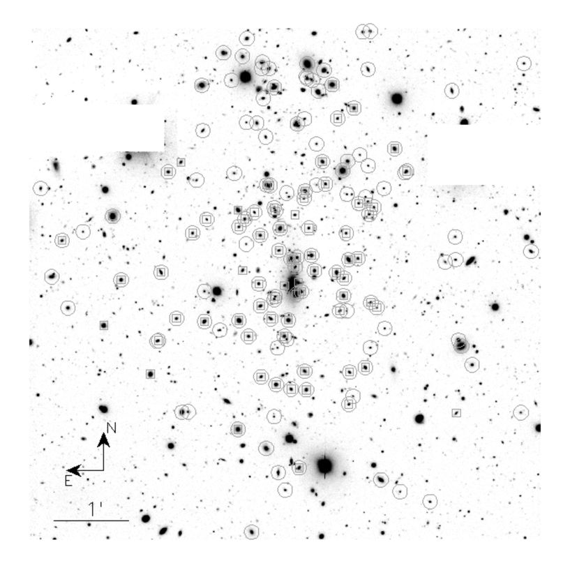
Figure 1: FORS1 R-band image of $\mathrm{MS\,1008}$. The image covers an area of $\sim 6.8\arcmin\times 6.8\arcmin$ around the cluster center. Galaxies included in the optical ($R$ and $I$ bands) and in the K-band samples are marked by circles and squares respectively.

We point out that the above selections allow us to obtain for each sample two sharp selection cuts in the space of structural parameters, i.e. the magnitude limit and the Sersic index cut. This is crucial for an accurate correction of PHP coefficients for selection effects (Section 4.2).

3 Derivation of Structural parameters

Structural parameters were derived for galaxies in the $R$-, $I$-, $K(S)$-   and $K(I)$-band images of $\mathrm{MS\,1008}$   by using the two-dimensional fitting method (see La Barbera et al. 2002 and references therein). The surface brightness of galaxies was modeled by the Sersic law (Sersic, 1968):

$$\mu(r)=\mu_{0}+2.5b_{n}\log\mathrm{e}\cdot(r/r_{\rm e})^{1/n},$$ (2)

where $b_{n}$ is a constant, defined in such a way that $r_{\rm e}$ is the effective (half-light) radius of the galaxy, r is the equivalent radius, $n$ is the Sersic index (shape parameter), and ${\mu_{0}}$ is the central surface brightness. The constant $b_{n}$ can be estimated by a power–law in $n$ (Ciotti & Bertin, 1999) with $b_{n}\sim 2n-1/3$ in first approximation (Capaccioli, 1989), or, with higher accuracy ($<1\%$), by the function $b_{n}\sim\exp[(0.6950+\ln n)-0.1789/n]$ (see LGM99). The mean surface brightness within ${r_{\rm e}}$, ${<\!\mu\!>_{\rm e}}$, is given by the following formula (e.g. Ciotti & Bertin 1999):

$$\begin{array}[]{lll}m_{\rm T}&=&-2.5\log(2\pi)+\mu_{0}-5\log(r_{\rm e})+\\ &&+5n\log b_{n}-2.5\log\Gamma(2n)\\ &=&-2.5\log(2\pi)-5\log(r_{\rm e})+<\!\mu\!>_{\rm e},\\ \end{array}$$ (3)

where $m_{\rm T}$ is the total magnitude of the galaxy and $\Gamma$ is the complete gamma function.

Galaxy images were fitted with seeing–convolved Sersic models, minimizing the function:

$$\mathrm{\chi^{2}=\sum_{i,j}\left[G_{i,j}-(bg+S\otimes PSF_{i,j})\right]^{2},}$$ (4)

where the symbol $\otimes$ denotes convolution, $G_{i,j}$ is the galaxy surface brightness at pixel $\left[i,j\right]$, $bg$ is the local background value, while $S$ and $PSF$ are the Sersic and the PSF models respectively. Seven output parameters were provided from the fitting process: the center coordinates, the effective radius, ${r_{\rm e}}$, the mean surface brightness, ${<\!\mu\!>_{\rm e}}$, the Sersic index, $n$, the position angle, $PA$, of major axis and the axis ratio, $b/a$. For each galaxy, neighbor objects were masked automatically using the ellipticity, position angle and isoarea parameters provided by running SExtractor (Bertin & Arnout, 1996) on the corresponding images. In the cases where SExtractor failed to provide reliable estimates of these parameters, such as in crowded regions and/or in the neighborhood of extended sources, masking was performed interactively. Very close galaxies were fitted simultaneously.

The PSFs of the $R$, $I$, $K(S)$  and $K(I)$  images were modeled by a sum of 2D Moffat functions, taking into account deviations of stellar isophotes from circular symmetry. Details on PSF modeling are given in Appendix A. Uncertainties on ${\log r_{\rm e}}$, ${<\!\mu\!>_{\rm e}}$  and $\log n$  were estimated by using numerical simulations and by comparing structural parameters among the different wavebands. Details can be found in Appendix B. Structural parameters for galaxies in the $R$-, $I$- and $K$-band samples are reported in Table 1. Since structural parameters turned out to be fully consistent between the $K(S)$  and $K(I)$  samples (see Appendix B), in Table 1 we report the averages of the $K(S)$  and $K(I)$  structural parameters, which were computed by weighting each value with the inverse square of the corresponding uncertainty.

Table 2: Acronyms used for fitting methods. Since the fit coefficients were corrected for selection effects (see Section 4.2), a prefix C was used for each acronym.

CLS${}_{\log r_{\rm e}}$	Corrected weighted least square fit with dependent variable ${\log r_{\rm e}}$.
CLS${}_{<\!\mu\!>_{\rm e}}$	Corrected weighted least square fit with dependent variable ${<\!\mu\!>_{\rm e}}$
CLSlogn	Corrected weighted least square fit with dependent variable $\log n$
$\rm CORLS$	Corrected orthogonal weighted least-square fit
$\rm CBLS$	Corrected bisector least square fit
$\rm CAMLS$	Corrected arithmetic mean of the least-square coefficients
$\rm CGMLS$	Corrected geometric mean of the least-square coefficients

4 Fitting the Photometric Plane

We derived the coefficients of the PHP by accounting for (i) selection effects, i.e. the cuts in Sersic index and magnitude; and (ii) the correlated uncertainties on structural parameters. Since different fitting methods are not equally affected by these effects (see La Barbera, Busarello, Capaccioli 2000, LBC00), the PHP coefficients were obtained for each sample by using different fitting methods, as described in Section 4.1. Correction for selection effects was performed by a Monte Carlo technique as detailed in Section 4.2.

4.1 Regression methods

The PHP coefficients were derived by using seven different fitting procedures: three weighted ordinary least-square fits, adopting as dependent variable one of the quantities ${\log r_{\rm e}}$, ${<\!\mu\!>_{\rm e}}$  and $\log n$; the orthogonal weighted least square fit, where the root mean square (rms) of residuals perpendicular to the plane are minimized; the bisector least square (BLS) fit (see LBC00); the arithmetic and the geometric means of the ordinary least-square coefficients. In the following, acronyms will be used for different fitting methods as summarized in Table 2.

In each fitting procedure, we derive the coefficients $a$, $b$ and $c$ of the plane (see Eq. 1) and its intrinsic dispersion $\sigma^{\rm i}$. For the ordinary and orthogonal least square fits, these quantities were derived by minimizing the following expression:

$$\begin{array}[]{rl}\chi^{2}=&-\ln L=\\ =&\sum_{k}\frac{r_{k}(a,b,c)^{2}}{\epsilon_{k}(a,b,c)^{2}+(\sigma^{i})^{2}}+1/2\ln\left[\epsilon_{k}(a,b,c)^{2}+(\sigma^{\rm i})^{2}\right],\end{array}$$ (5)

where $L$ is the likelihood function, $r_{k}$ are the residuals about the plane, $\epsilon_{k}$ are the uncertainties on $r_{k}$, and $\sigma^{\rm i}$ is the intrinsic dispersion of the PHP along the direction, $\mn@boldsymbol{d}_{\rm min}$, where residuals are minimized. The terms $\epsilon_{k}$ are the uncertainties on $r_{k}$ and were obtained by projecting the covariance matrix of measurement errors on structural parameters along $\mn@boldsymbol{d}_{\rm min}$. We point out that although this procedure allows each point to be weighted with the corresponding uncertainties, it does not correct exactly for biases on fitting procedures which are due to the correlation among such uncertainties. It is always possible, in fact, to vary the covariance matrix of measurement errors on ${\log r_{\rm e}}$, ${<\!\mu\!>_{\rm e}}$  and $\log n$, without changing its projection on a given direction $\mn@boldsymbol{d}_{\rm min}$. In order to estimate the amount of bias which is due to the correlation of the uncertainties, we adopted the MIST fits (LBC00) which provides unbiased values of ordinary least-square coefficients by using the mean covariance matrix of uncertainties on the three variables. The bias turned out to be always smaller than $5\%$ for each sample, and therefore we did not apply corrections for this effect. In order to derive the quantities $a$, $b$, $c$ and $\sigma^{\rm i}$, we minimized Eq. 5 by using a Levenberg-Marquardt algorithm. For what concerns the $\rm CBLS$, $\rm CAMLS$  and $\rm CGMLS$  fits, the PHP coefficients were calculated from those of the CLS fits. For this reason, a different weight is given to each galaxy also in these fitting methods. Uncertainties on $a$, $b$, $c$ and $\sigma^{\rm i}$ were estimated by the bootstrap method, applying $N=2500$ bootstrap iterations.

4.2 Selection effects

Selection effects were corrected for by using numerical simulations, producing distributions of points in the space of structural parameters which resembled those of real galaxies. Points in each simulation were generated as follows. Magnitudes were assigned according to the luminosity function, which was modeled as a Schechter function with slope $\alpha$ and characteristic magnitudes $M^{\star}$. The values of $\alpha$ and $M^{\star}$ were drawn from Busarello et al. (2002) for the $R$ and $I$ bands, and from de Propris et al. (1999) for the $K$ band. Effective radii and mean surface brightnesses were obtained according to the luminosity-size relation, whose slopes, zero-point and scatter were derived from the data of $\mathrm{MS\,1008}$. Sersic indices were assigned using the PHP coefficients, $a$, $b$ and $c$, and its $\log n$  scatter, $\sigma_{\log n}$. The values of $a$, $b$, $c$ and $\sigma_{\log n}$  were chosen by an iterative procedure. For each iteration, a simulated distribution in the space of structural parameters was constructed by imposing the same selection effects, i.e. the magnitude and Sersic index cuts, of the real samples, and the PHP coefficients were computed by using all the fitting methods described in Section 4.1. The values of $a$, $b$, $c$ and $\sigma_{\log n}$were modified until the coefficients derived from the simulated samples matched those of the real samples for $\it all$ the fitting methods. This procedure allowed us to achieve an excellent match, with an accuracy better than $\sim 5\%$ for all the fitting coefficients. Once the values of $a$, $b$, $c$ and $\sigma_{\log n}$  were chosen, we estimated the relative variations of PHP coefficients of all the regression methods after selection cuts were removed from the simulated samples. The variations were used as correction factors for the PHP coefficients of $\mathrm{MS\,1008}$. As an example, in Table 3 we report the correction factors for the $R$-band sample of $\mathrm{MS\,1008}$. We see that the bias can be as large as $\sim-35\%$ for the coefficient $a$ of the CLS_logn fit, and that it strongly depends on the fitting method, being smaller than $\sim 10\%$ in absolute value for the $\rm CORLS$, $\rm CBLS$  and $\rm CAMLS$  fits. The uncertainties on the correction factors were estimated by changing the input parameters of the simulation algorithm (e.g. the value of $\alpha$) according to their uncertainties, and repeating the iteration procedure. We found that the bias on the PHP coefficients varies at most by $\sim 4\%$ for the coefficient $a$ in the $\rm CLS$  fits. This is smaller with respect to the typical uncertainties on PHP coefficients, and was therefore neglected.

Table 3: Bias on the $R$-band PHP coefficients due to selection effects.

	$\frac{\delta a}{a}$	$\frac{\delta b}{b}$	$\frac{\delta c}{c}$	$\frac{\delta\sigma_{\log r_{\rm e}}}{\sigma_{\log r_{\rm e}}}$	$\frac{\delta\sigma_{\log r_{\rm e}}^{\rm i}}{\sigma_{\log r_{\rm e}}^{\rm i}}$
CLS${}_{\log r_{\rm e}}$	0.22	-0.07	-0.02	0.12	0.08
CLS${}_{<\!\mu\!>_{\rm e}}$	0.33	0.08	0.09	0.18	0.16
CLSlogn	-0.35	0.08	-0.01	-0.16	-0.03
$\rm CORLS$	-0.10	-0.01	-0.03	0.02	0.09
$\rm CBLS$	0.10	0.00	0.01	0.11	0.12
$\rm CAMLS$	0.02	0.03	0.03	0.09	0.12
$\rm CGMLS$	0.19	0.03	0.05	0.11	0.08

We point out that the correction procedure was repeated independently for each waveband of $\mathrm{MS\,1008}$, without making any assumption a priori on how the properties of galaxies in the space of structural parameters can vary among the different wavebands.

Table 4: Coefficients of the PHP in the $R$ band.

	$a$	$b$	$c$	$\sigma_{\log r_{\rm e}}$	$\sigma_{\log r_{\rm e}}^{\rm i}$
CLS${}_{\log r_{\rm e}}$	$1.00\pm 0.09$	$0.184\pm 0.010$	$-4.70\pm 0.21$	$0.17\pm 0.01$	$0.15\pm 0.01$
CLS${}_{<\!\mu\!>_{\rm e}}$	$0.90\pm 0.14$	$0.303\pm 0.019$	$-7.07\pm 0.38$	$0.21\pm 0.02$	$0.19\pm 0.03$
CLSlogn	$1.40\pm 0.16$	$0.157\pm 0.025$	$-4.22\pm 0.40$	$0.18\pm 0.02$	$0.16\pm 0.02$
$\rm CORLS$	$1.10\pm 0.11$	$0.175\pm 0.012$	$-4.48\pm 0.22$	$0.16\pm 0.01$	$0.14\pm 0.01$
$\rm CBLS$	$1.07\pm 0.06$	$0.219\pm 0.009$	$-5.41\pm 0.19$	$0.17\pm 0.01$	$0.14\pm 0.01$
$\rm CAMLS$	$1.09\pm 0.08$	$0.215\pm 0.010$	$-5.34\pm 0.20$	$0.17\pm 0.01$	$0.15\pm 0.01$
$\rm CGMLS$	$1.07\pm 0.09$	$0.201\pm 0.017$	$-5.04\pm 0.34$	$0.17\pm 0.01$	$0.15\pm 0.01$

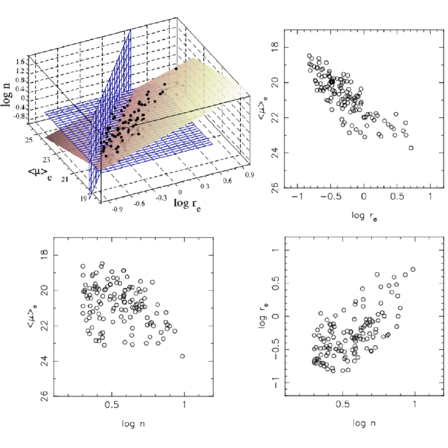
Figure 2: PHP of $\mathrm{MS\,1008}$   in the R-band. The upper–left panel shows a 3D view of the plane, where black circles mark positions of galaxies ($\rm N=129$) in the space of structural parameters. The shaded surface is the PHP, as defined by the $\rm CBLS$  fitting method, while the vertical and horizontal blue grids depict the selection cuts in magnitude and Sersic index respectively. The shading is realized in such a way that color intensities are inversely proportional to $\log n$. Note that the plot of the PHP is transparent, and therefore black points below the surface appear as partly obscured symbols. The upper–right and the lower panels show the ${\log r_{\rm e}}$–${<\!\mu\!>_{\rm e}}$, $\log n$–${<\!\mu\!>_{\rm e}}$  and $\log n$–${\log r_{\rm e}}$  projections of the PHP.

5 Photometric Planes of $\mathrm{MS\,1008}$

The distribution of galaxies in the space of structural parameters is shown in Fig. 2, where we show the distribution of galaxies in the ${\log r_{\rm e}}$–${<\!\mu\!>_{\rm e}}$, $\log n$–${<\!\mu\!>_{\rm e}}$  and $\log n$–${\log r_{\rm e}}$  planes, and a 3D view of the PHP, with the corresponding magnitude and Sersic index cuts represented by two orthogonal planes. An edge projection of the plane is also shown in Fig. 3. We see that galaxies follow a well-defined PHP at $z=0.3$, with Sersic indices that increase towards lower surface brightness values and larger effective radii.

The coefficients of the PHP in the $R$, $I$ and $K$ bands for the different fitting procedures are reported in Tables 4, 5 and 6 respectively, together with the estimate $\sigma_{\log r_{\rm e}}^{\rm i}$ of the intrinsic dispersion in ${\log r_{\rm e}}$  about the plane. All these values were corrected for selection effects as detailed in Section 4.2. The $K$-band coefficients were obtained by combining the values obtained for the $K(S)$and $K(I)$  bands, as discussed below (Section 5.2). For the $\rm CLS$  and $\rm CORLS$  fits, the quantity $\sigma_{\log r_{\rm e}}^{\rm i}$ was estimated by projecting $\sigma^{\rm i}$ in Eq. 5 along the direction $\mn@boldsymbol{\log}r_{\rm e}$, while for the other fitting procedures we subtracted in quadrature to the rms of ${\log r_{\rm e}}$  residuals the amount of scatter due to measurement errors. This was performed by taking into account the correlation of uncertaintities on ${\log r_{\rm e}}$, ${<\!\mu\!>_{\rm e}}$  and $\log n$.

By looking at Tables 4, 5 and 6, we see that (i) the coefficients of the PHP obtained by the various fitting procedures are significantly different, and (ii), whatever the regression method is, the PHP has significant intrinsic dispersion. As discussed by LBC00 for the FP relation, the existence of intrinsic scatter for a bivariate relation and our ignorance on its origin imply that different fitting methods do not necessarily provide consistent results. We note, however, that the dependence of PHP coefficients on the fitting procedure is particularly significant only for the CLS regressions, which give a special role to the variable whose residuals are minimized during the fit. On the other hand, treating equally all the variables, as in the CORLS, CBLS, CAMLS and CGMLS fits, gives much more robust estimates, allowing us to obtain a stable determination of PHP coefficients. We also note that the CLS${}_{<\!\mu\!>_{\rm e}}$ regression provides a lower value of $a$ and a higher value of $b$ with respect to the CLS${}_{\log r_{\rm e}}$ method. On the contrary, the CLS_logn regression produces a higher value of $a$ and a lower value of $b$ with respect to the CLS${}_{\log r_{\rm e}}$ fit. Since the CBLS, CAMLS and CGMLS fits are based on an average of the CLS coefficients, the corresponding coefficients are very close to those of the CLS${}_{\log r_{\rm e}}$ method. Since the coefficients of the bisector fit have a smaller relative uncertainties with respect to the other fitting methods, we will refer to these coefficients in the following analysis (Section 6.2). It is also interesting to note that the correction for selection effects is negative for the $\rm CORLS$  fit while it is positive for the $\rm CBLS$, $\rm CAMLS$  and $\rm CGMLS$  regressions, and that, therefore, if selection effects would have not taken into account, the difference among the $\rm CORLS$  and the $\rm CBLS$, $\rm CAMLS$  and $\rm CGMLS$  fits would have been significant.

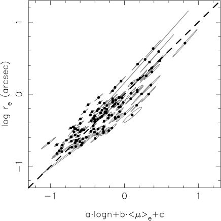
Figure 3: Edge-on view of the $R$-band PHP of $\mathrm{MS\,1008}$. The plot shows the $N=129$ galaxies of the $R$-band sample. Ellipses denote uncertainties on structural parameters and correspond to $1\sigma$ confidence contours.

5.1 The PHP in optical wavebands

A proper comparison of PHP coefficients between different samples has to account for the fact that their uncertainties are correlated. For this reason, we chose to compare simultaneously the slopes $a$ and $b$ of the PHP and one slope, $a$, with its zeropoint $c$. The comparison of $b$ versus $c$ as well as other plots with pairs of quantities from Tables 4 and 5 do not add further information to the discussion and are not shown in the following. In Fig. 4, we plot the $R$- and $I$- band coefficients. Taking into account the mean galaxy colour, $\overline{R\!-\!I}\sim 0.75$ at $z\sim 0.3$, we expect an offset between the $I$- and $R$- band PHP zero-points of $\Delta_{R-I}\sim b\cdot\overline{R\!-\!I}$. In order to remove this effect from the comparison, we subtracted the quantity $\Delta_{R-I}$ from the I- band values of $c$ which are shown in Fig. 4. We note that since the value of $\Delta_{R-I}$ is proportional to $b\sim 0.2$, uncertainties on $\overline{R\!-\!I}$ do not affect the comparison in Fig. 4.

As shown in the figure, the PHP coefficients are fully consistent between the $R$ and $I$ bands. This is clearly in agreement with the fact that structural parameters do not show significant variations among optical wavebands (see Appendix B), and is due to the fact that the $R$ and $I$ bands at $z=0.3$ sample a very similar spectral region, where differences in stellar population properties of galaxies, such as their internal colour gradients and the colour magnitude relation, are negligible. For what concerns the dispersion around the plane, we see from Tables 4 and 5 that this is also consistent between the $R$ and $I$ bands, amounting on average to $\sim 0.18$ dex ($\sim 41\%$) in ${\log r_{\rm e}}$. The same result holds for the intrinsic dispersion of the PHP, which amounts to $\sim 0.14-0.15$ dex ($\sim 32-35\%$) in ${\log r_{\rm e}}$. We note that although for the CLS${}_{<\!\mu\!>_{\rm e}}$ and CLS_logn fits the value of $\sigma^{\rm i}_{\log r_{\rm e}}$  is slightly larger with respect to that of the other fitting methods, the corresponding uncertainties of $\sigma^{\rm i}_{\log r_{\rm e}}$  are larger, making this difference not particularly significant. We also note that only a few percent of the observed dispersion about the PHP are explained by the the measurement errors on ${\log r_{\rm e}}$, ${<\!\mu\!>_{\rm e}}$  and $\log n$. As shown in Fig. 3, in fact, uncertainties on structural parameters are strongly correlated in a direction which is almost parallel to the PHP.

We also analyzed the presence of a possible curvature in the distribution of ETGs in the space of ${\log r_{\rm e}}$, ${<\!\mu\!>_{\rm e}}$  and $\log n$, by considering correlations among ${\log r_{\rm e}}$  residuals about the plane and each of the three variables. We found that such correlations are very weak, the Spearman’s rank coefficients amounting to 0.14 for the correlation between residuals and ${\log r_{\rm e}}$, and to -0.2 for the other correlations with ${<\!\mu\!>_{\rm e}}$  and $\log n$. These coefficients can be easily explained by the selection cuts in the space of structural parameters. We also fitted the $R$-band PHP by using ${\log r_{\rm e}}$  as dependent variable and by adding to Eq. 1 one among all the possible quadratic terms which can be constructed from the two quantities ${<\!\mu\!>_{\rm e}}$  and $\log n$. All these terms were found to be consistent with zero at the level of $1.4\sigma$, the ${\log r_{\rm e}}$  scatter of the PHP decreasing by less than $1\%$ in each case. Our data, therefore, indicate that there is no significant departure of the PHP from a flat relation.

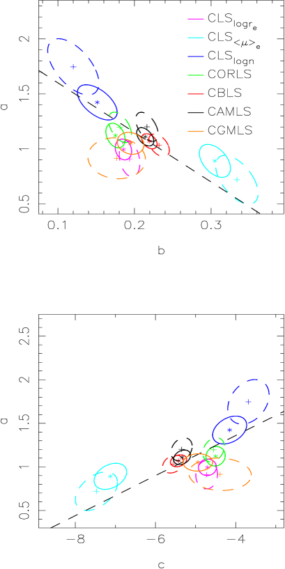
Figure 4: Comparison of the optical PHP coefficients. The $R$- and $I$- band coefficients are marked by asterisks and crosses respectively, while the fitting procedure are shown in different colors, as indicated in the upper panel. The solid (dashed) ellipses mark $1\sigma$ confidence contours for each pair of R(I)-band coefficients (see text). The dashed lines in the upper and lower panels show the direction of the mean correlation of uncertainties on $a$ and $b$, and $b$ and $c$ respectively.

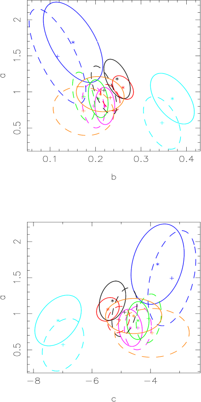
Figure 5: The same of Fig. 4 for the $K(S)$  and $K(I)$  coefficients. Asterisks and crosses mark the $K(S)$  and $K(I)$  PHP coefficients respectively. Ellipses denote $1.5\sigma$ confidence contours.

Table 5: Coefficients of the PHP in the $I$ band.

	$a$	$b$	$c$	$\sigma_{\log r_{\rm e}}$	$\sigma_{\log r_{\rm e}}^{\rm i}$
CLS${}_{\log r_{\rm e}}$	$0.90\pm 0.15$	$0.194\pm 0.013$	$-4.73\pm 0.25$	$0.18\pm 0.01$	$0.14\pm 0.01$
CLS${}_{<\!\mu\!>_{\rm e}}$	$0.75\pm 0.20$	$0.331\pm 0.026$	$-7.32\pm 0.51$	$0.22\pm 0.02$	$0.20\pm 0.02$
CLSlogn	$1.66\pm 0.24$	$0.124\pm 0.029$	$-3.70\pm 0.46$	$0.25\pm 0.04$	$0.10\pm 0.05$
$\rm CORLS$	$1.19\pm 0.13$	$0.182\pm 0.015$	$-4.53\pm 0.26$	$0.19\pm 0.02$	$0.14\pm 0.01$
$\rm CBLS$	$1.03\pm 0.09$	$0.232\pm 0.013$	$-5.52\pm 0.24$	$0.19\pm 0.01$	$0.15\pm 0.01$
$\rm CAMLS$	$1.17\pm 0.12$	$0.218\pm 0.014$	$-5.33\pm 0.24$	$0.20\pm 0.01$	$0.16\pm 0.01$
$\rm CGMLS$	$0.95\pm 0.16$	$0.186\pm 0.025$	$-4.55\pm 0.51$	$0.19\pm 0.02$	$0.15\pm 0.02$

Table 6: Coefficients of the PHP in the $K$ band.

	$a$	$b$	$c$	$\sigma_{\log r_{\rm e}}$	$\sigma_{\log r_{\rm e}}^{\rm i}$
CLS${}_{\log r_{\rm e}}$	$0.83\pm 0.13$	$0.209\pm 0.010$	$-4.51\pm 0.19$	$0.18\pm 0.01$	$0.15\pm 0.02$
CLS${}_{<\!\mu\!>_{\rm e}}$	$0.75\pm 0.17$	$0.351\pm 0.020$	$-6.83\pm 0.32$	$0.21\pm 0.02$	$0.17\pm 0.02$
CLSlogn	$1.39\pm 0.29$	$0.151\pm 0.033$	$-3.51\pm 0.39$	$0.27\pm 0.05$	$0.23\pm 0.05$
$\rm CORLS$	$0.90\pm 0.14$	$0.192\pm 0.010$	$-4.18\pm 0.19$	$0.19\pm 0.01$	$0.17\pm 0.02$
$\rm CBLS$	$0.97\pm 0.08$	$0.245\pm 0.010$	$-5.13\pm 0.17$	$0.20\pm 0.01$	$0.15\pm 0.02$
$\rm CAMLS$	$1.00\pm 0.15$	$0.235\pm 0.013$	$-4.98\pm 0.19$	$0.21\pm 0.02$	$0.19\pm 0.02$
$\rm CGMLS$	$0.91\pm 0.13$	$0.212\pm 0.027$	$-4.57\pm 0.49$	$0.19\pm 0.02$	$0.16\pm 0.02$

5.2 The $K$-band plane

In order to derive the PHP of $\mathrm{MS\,1008}$   in the $K$ band we applied separately the different fitting procedures to the $K(S)$  and $K(I)$  structural parameters. The comparison of the $K(S)$  and $K(I)$  coefficients is shown in Fig. 5, where the same quantities as Fig. 4 are shown. The important outcome is that the PHP coefficients of the NIR samples are fully consistent, with a confidence level $\sol 1.5\sigma$. The same result holds for the dispersion around the plane. This is a reassuring result since the $K(S)$  and $K(I)$  parameters were obtained from images with different resolution and seeing.

Since the coefficients and dispersions of the $K(S)$  and $K(I)$  PHPs turned out to be consistent, we combined their values by a weighted mean. The resulting coefficients are shown in Table 6.

6 PHP dependence on waveband and redshift

6.1 The PHP in optical and NIR wavebands

The $R$- and $K$- band coefficients of the PHP are shown in Fig. 6. In order to remove the mean galaxy colour from the comparison, we proceeded as in Section 5.1 by subtracting from the coefficient $c$ in the $K$ band the term $\Delta_{R-K}=-b\cdot\overline{R\!-\!K}$, with $\overline{R-K}\sim 3.2$ at $z\sim 0.3$. Since the $I$-band coefficients are consistent with those in the $R$ band, they do not add further information to the discussion and are not shown in the figure. By looking at Fig. 6 and at Tables 4, 5 and 6, we see that, whatever regression method is adopted, the PHP coefficients turn out to be fully consistent among the optical and NIR wavebands. We note that since the Sersic index and the magnitude cuts affect each fitting procedure in a different way, the independence of the above result on the fitting method makes it very robust with respect to selection effects in the samples. Considering the $\rm CORLS$, $\rm CBLS$, $\rm CAMLS$  and $\rm CGMLS$  fits, we find $a\sim 1$ and $b\sim 0.2$ both in the optical and NIR wavebands. We also note that the intrinsic scatter about the $K$-band plane is fully consistent with the value of $\sim 0.14-0.15$ dex found for the optical PHP, provided that measurement uncertainties are taken into account.

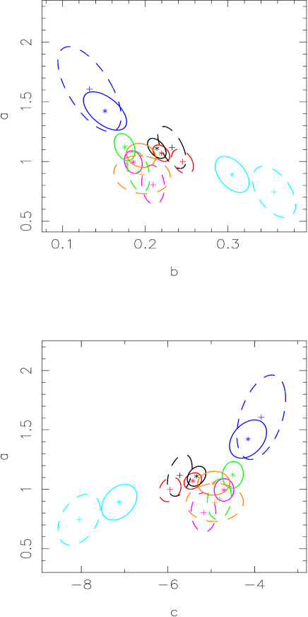
Figure 6: Comparison of the PHP coefficients for the $R$ and $K$ bands (asterisks and crosses respectively). Solid (dashed) ellipses denote $1\sigma$ confidence contours for R(K)-band coefficients.

6.2 The PHP at $z\sim 0.3$ and $z\sim 0$

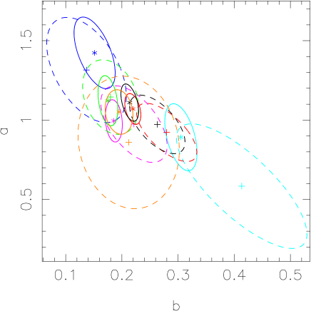
Figure 7: Comparison of the $R$-band PHP slopes of $\mathrm{MS\,1008}$   (crosses) with those of nearby galaxies in the $B$ band from GRA02 (asterisks). Ellipses denote $1.5\sigma$ confidence contours.

In order to address the redshift dependence of the PHP, we compared our results with those of GRA02, who derived the PHP at $z\sim 0$ by using $B$-band structural parameters for $N=38$ ETGs in the Virgo and Fornax clusters. We note that the $R$ band at $z=0.3$ is closed to $B$-band restframe, and therefore the data of GRA02 and those of $\mathrm{MS\,1008}$   cover approximately the same restframe wavelengths. To perform a homogeneous comparison, we used the data in table 1 of GRA02 and re-derived the PHP coefficients using the regression methods described in Section 4.1. Selection effects were taken into account by constructing PHP simulations as described in Section 4.2 with the same magnitude and Sersic index cuts as the GRA02 sample, i.e. $B=15$ and $n=1.5$, respectively. We note that, since the GRA02 sample is not complete in any sense (see sec. 2 of GRA02), the above procedure provides only a rough correction of the selection biases. Because of the wide magnitude range of the GRA02 sample ($\sim 5.3$ mag), the corrections turned out to be quite small, amounting to $5\%$ on average, and to at most $10\%$ for the coefficient $a$ in the CLS_logn fit. The bias corrected PHP coefficients at $z\sim 0$ are given in Table 7. The intrinsic dispersion of the PHP was computed assuming a typical uncertainty of $\sim 0.1$ dex in $\log n$  (see sec. 2 of GRA02), and adopting as mean covariance matrix of uncertainties on structural parameters that of galaxies in $\mathrm{MS\,1008}$, which was re-scaled to match the uncertainty on $\log n$  at $z\sim 0$. The slopes of the PHP obtained by the $\rm CORLS$, $\rm CBLS$, $\rm CAMLS$  and $\rm CGMLS$  fits can be compared with the values of $a=0.89\pm 0.14$ and $b=0.24\pm 0.036$, that were derived from GRA02 by the bisector fit, treating equally all the three variables. The values in Table 7 are fully consistent with those of GRA02. The PHP slopes of the GRA02 sample and those of $\mathrm{MS\,1008}$   are compared in Fig. 7, where we see that the values of a and b at $z\sim 0$ are fully consistent with those at $z\sim 0.3$. We note that due to the smaller sample size at $z\sim 0$ the corresponding uncertainties on a and b are larger, particularly for some of the fitting procedures (e.g. the CLS${}_{<\!\mu\!>_{\rm e}}$ fit). As shown in Table 7, the intrinsic dispersion around the plane does not change significantly, provided that measurement uncertainties are taken into account.

Table 7: $B$-band coefficients of the PHP for the GRA02 sample.

	$a$	$b$	$c$	$\sigma_{\log r_{\rm e}}$	$\sigma_{\log r_{\rm e}}^{\rm i}$
CLS${}_{\log r_{\rm e}}$	$0.97\pm 0.16$	$0.221\pm 0.039$	$-4.87\pm 0.80$	$0.17\pm 0.01$	$0.14\pm 0.02$
CLS${}_{<\!\mu\!>_{\rm e}}$	$0.58\pm 0.27$	$0.433\pm 0.078$	$-9.00\pm 1.55$	$0.20\pm 0.04$	$0.17\pm 0.04$
CLSlogn	$1.31\pm 0.24$	$0.135\pm 0.052$	$-3.18\pm 0.98$	$0.21\pm 0.04$	$0.15\pm 0.03$
$\rm CORLS$	$1.14\pm 0.15$	$0.180\pm 0.031$	$-4.07\pm 0.64$	$0.19\pm 0.02$	$0.14\pm 0.01$
$\rm CBLS$	$0.92\pm 0.12$	$0.279\pm 0.036$	$-5.92\pm 0.71$	$0.17\pm 0.01$	$0.13\pm 0.01$
$\rm CAMLS$	$0.97\pm 0.12$	$0.263\pm 0.034$	$-5.58\pm 0.66$	$0.17\pm 0.01$	$0.13\pm 0.01$
$\rm CGMLS$	$0.85\pm 0.30$	$0.212\pm 0.060$	$-4.45\pm 1.25$	$0.18\pm 0.05$	$0.16\pm 0.06$

Taking advantage of the fact that the PHP slopes are consistent between $z\sim 0$ and $z\sim 0.3$, we re-computed the coefficient $c$ at $z\sim 0$ and $z\sim 0.3$ by fixing the slopes of the PHP to the values of $a$ and $b$ obtained for $\mathrm{MS\,1008}$   by the $\rm CBLS$  fit, i.e. $a=1.07$ and $b=0.219$. The $\rm CBLS$  fit was chosen because of the smaller uncertainties of bisector coefficients with respect to those of other fitting procedures. The value of $c$ at $z\sim 0$ was also corrected for magnitude and Sersic index cuts as described in Section 4.2. Due to the robustness of the $\rm CBLS$  regression with respect to selection effects (see Table 3), the correction turned out to be very small ($\sim 0.2\%$). The coefficient $c$ amounts to $-4.737\pm 0.028$ at $z\sim 0$ and $-5.337\pm 0.014$ for $\mathrm{MS\,1008}$, differing by $\Delta(c)=-0.60\pm 0.03$. The value of $\Delta(c)$ can be analyzed by taking the average of the difference between the PHP equations (Eq. 1) at $z\sim 0.3$ and $z\sim 0$:

$$\Delta(c)=\Delta(\overline{\log r_{\rm e}})-a\cdot\Delta(\overline{\log n})-b\cdot\Delta(\overline{<\!\mu\!>_{\rm e}}).$$ (6)

Assuming that, on average, structural parameters vary from $z\sim 0$ to $z\sim 0.3$ only because of the luminosity evolution of stellar populations, we can re-write the previous equation by setting $\Delta(\overline{\log r_{\rm e}})=0$ and $\Delta(\overline{\log n})=0$ (see discussion in Section 7.4):

$$\Delta(c)=-\log(d_{\rm A})-b\cdot\left[10\Delta\left[\log\left(\frac{1+z}{1.008}\right)\right]-(B_{0.0}-R_{0.3})\right],$$ (7)

where the term $10\Delta\left[\log\left(\frac{1+z}{1.008}\right)\right]$ accounts for the surface brightness dimming between the redshift of $\mathrm{MS\,1008}$ and that of the GRA02 sample, $d_{\rm A}$ is the angular diameter distance corresponding to $z=0.306$, while $(B_{0.0}-R_{0.3})$ is the difference between the $B$ magnitude at $z\sim 0$ and the $R$-band magnitude at $z\sim 0.3$. Eq. 7 was used to compare the measured value of $\Delta(c)$ with predictions of stellar population models from the GISSEL03 code (Bruzual & Charlot, 2003). We considered two different stellar population models with solar metallicity and a Scalo IMF (Scalo, 1986), the first one being a simple stellar population (SSP), the second one having an exponentially declining star formation rate with time scale $\tau=1~{}Gyr$. For both models, we computed the value of $\Delta(c)$ from Eq. 7 by deriving the $B$- and $R$- band magnitudes at $z=0$ and $z=0.306$ respectively, for different formation redshifts $z_{\rm f}$. In Fig. 8, we show the values of $\Delta(c)$ for the two stellar populations as a function of $z_{\rm f}$. The measured value of $\Delta(c)$ is marked by the dash–dotted line in the plot, while the hatched area is the confidence interval defined by measurement uncertainties on $\Delta(c)$. The figure shows that both models cross the hatched region and are consistent, therefore, with the measured value of $\Delta(c)$. The crossing points define lower limits for the formation redshift of galaxy stellar populations. For the SSP and $\tau=1~{}Gyr$ models, we obtain $z_{\rm f}>1$ and $z_{\rm f}>2$ respectively.

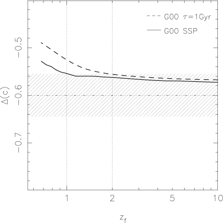
Figure 8: The difference of the PHP zero-point, $\Delta(c)$, between $z=0.3$ and $z=0$ is compared with predictions of stellar population models. The dash-dotted line and the gray hatched region indicate the mean value of $\Delta(c)$ and the corresponding $\pm 1.5\sigma$ confidence interval. The dotted lines mark the intersections of the two models with the hatched area.

7 Discussion

We have shown that cluster ETGs at $z\sim 0.3$   follow a tight correlation among ${\log r_{\rm e}}$, ${<\!\mu\!>_{\rm e}}$  and $\log n$, with an intrinsic dispersion of $\sim 32\%$ in ${r_{\rm e}}$. Our data indicate that the PHP has no significant curvature. In Section 7.1 we discuss whether stellar populations can be the origin of the intrinsic dispersion about the plane, while in Section 7.2 we attempt to find a possible explanation for the absence of curvature in the PHP. Sections 7.3 and 7.4 deal with the waveband and redshift dependence of the PHP coefficients.

7.1 The intrinsic dispersion of the PHP

In Section 5 we showed that the PHP relation has significant intrinsic dispersion, amounting to $\sigma^{\rm i}_{\log r_{\rm e}}\sim 0.14$ dex ($\sim 32\%$) both in optical and NIR wavebands. This dispersion is fully consistent with that found by GRA02 for ETGs in nearby clusters. The intrinsic scatter of the PHP turns out, therefore, to be larger with respect to that of the FP (see values reported in Section 1), although it is smaller with respect to that of other correlations among galaxy parameters. For example, Pahre, Djorgovski & de Carvalho (1998) analyzed different correlations among photometric and spectroscopic properties of nearby ETGs. They found that the Kormendy relation (KR) and the $\rm Mg_{2}$ FP have a ${\log r_{\rm e}}$  scatter of $\sim 0.23$ dex and $\sim 0.17$ dex respectively, where the $\rm Mg_{2}$ FP relation was constructed by replacing the velocity dispersion term in the FP with the $\rm Mg_{2}$ line–strength. It is interesting to compare these values with those we can obtain for $\mathrm{MS\,1008}$. A KR fit to the $R$-band sample of $\mathrm{MS\,1008}$   gives a ${\log r_{\rm e}}$  dispersion of $\sim 0.2$ dex, that is $\sim 14\%$ higher than the scatter of the PHP. This result is consistent with what found by LMB04. Since we do not have $\rm Mg_{2}$ line–strengths, we constructed a ‘photometric’ FP by replacing velocity dispersions with optical-NIR galaxy colours (see e.g. de Carvalho & Djorgovski 1989). Using $I\!-\!K$ colours available for $N=105$ galaxies from the $R$-band sample of $\mathrm{MS\,1008}$, we obtain $\log r_{\rm e}\propto(0.25\pm 0.02)\cdot<\!\mu\!>_{\rm e}+(0.23\pm 0.07)\cdot(I\!-\!K)$, with a ${\log r_{\rm e}}$  rms of $0.175$ dex, which is $\sim 8\%$ larger with respect to the PHP, but significantly smaller with respect to the KR. Since effective parameters turn out to correlate with both colours and Sersic indices, we also tried to construct a photometric hyperplane with ${\log r_{\rm e}}$, ${<\!\mu\!>_{\rm e}}$, $\log n$  and   $I\!-\!K$. We found, however, that the $I\!-\!K$ term in such a hyperplane is only marginally significant ($1.5\sigma$), and that the scatter about the relation decreases only by $1\%$ with respect to that of the PHP. This result is also shown in Fig. 9, where we plot ${\log r_{\rm e}}$  residuals about the PHP versus residuals from the $I\!-\!K$ vs. $K$ CM relation of $\mathrm{MS\,1008}$. Such $\delta-\delta$ diagrams have been already applied in several works to investigate the origin of residuals about the FP (e.g. Prugniel & Simien 1996). The plot clearly shows that there is no correlation among residuals to the PHP and CM relations, the corresponding Spearman’s rank coefficient amounting to $-0.12\pm 0.09$. This implies that either the scatter of the PHP does not origin from stellar population parameters or that a complex combined effect of such parameters (e.g. age and metallicity) is acting in such a way that no correlation appears in the $\delta$–$\delta$ diagram. This issue could be addressed by correlating PHP residuals with line–strength indices.

Figure 9: Relation among residuals to the CM and PHP relations.

7.2 Why a plane with ${\log r_{\rm e}}$, ${<\!\mu\!>_{\rm e}}$  and $\log n$?

As mentioned in Section 1, MLC00 and MLC01 found that ETGs populate a curved manifold in the space of structural parameters, showing that the existence of such a PHP can be explained by the specific entropy of ETGs, $s$, being an increasing function of their mass, $M$. MLC01 also showed that the existence of a plane in the space of ${\log r_{\rm e}}$, ${\mu_{0}}$   and $\log n$  can be explained by the limited range considered for $\log n$ in previous works (with $\log n\sog 0.15$, see fig. 10 of MLC01). Since the variables used by MLC01 as well as the quantities ${\log r_{\rm e}}$, ${\mu_{0}}$   and $\log n$  are not linearly related to ${\log r_{\rm e}}$, ${<\!\mu\!>_{\rm e}}$  and $\log n$  (see Section 1), an intriguing question arises on what the origin is of the flatness of the PHP in the ${\log r_{\rm e}}$, ${<\!\mu\!>_{\rm e}}$  and $\log n$  space.

To address this issue, we tried to understand if there is some simple relation between the specific entropy of ETGs and the three quantities ${\log r_{\rm e}}$, ${<\!\mu\!>_{\rm e}}$  and $\log n$. This was achieved by considering the same galaxy models described in MLC00 and MLC01, that is spherical, non-rotating systems, with negligible radial gradients of the mass-to-light ratio (i.e. one component models). We point out that attempting to derive an interpretation for the existence of the PHP on the basis of more complex models is well beyond the scope of the present work, and therefore we do not discuss further here the above mentioned hypotheses. As detailed in Appendix C, it can be shown that the specific entropy is given by the following formula:

$$\begin{array}[]{lll}s&=&0.5\ln\!10\cdot\log M/L+2.5\ln\!10\cdot\log r_{\rm e}+\\ &-&0.2\ln\!10<\!\mu\!>_{\rm e}+\Phi(n)+const.\end{array}$$ (8)

where $\Phi(n)$ is an dimensionless function given by:

$$\begin{array}[]{lll}\Phi(n)&=&0.5\ln\left(\frac{b_{n}^{2n}}{n\Gamma(2n)}\right)+\\ &+&2\frac{b_{n}^{2n}}{n\Gamma(2n)}\cdot\int\tilde{\rho}\ln\left(\tilde{P}^{3/2}\tilde{\rho}^{-5/2}\right)d\!s,\end{array}$$ (9)

$\tilde{P}$ and $\tilde{\rho}$ being the dimensionless 3D pressure and density profiles of the models respectively. Since $\Phi(n)$ is a very complex function of the Sersic index, there is no a priori reason for which a systematic variation of $s$ along the galaxy sequence (such as the $s$–$M$ relation found by MLC00) should imply the existence of a plane in the space of ${\log r_{\rm e}}$, ${<\!\mu\!>_{\rm e}}$  and $\log n$. From Eq. 8, we see that this is the case only and only if the function $\Phi(n)$ is a linear function of $\log n$. In Fig. 10 we plot the function $\Phi(n)$ for different values of $\log n$. The values of $\Phi(n)$ were computed numerically, by using the formulae in Appendix C. By looking at the figure, it is remarkable to note that there exists almost an exact linear relation between $\Phi(n)$ and $\log n$. A linear best-fit gives $\Phi(n)\sim 0.988\cdot\log(n)+1.57$, with residuals smaller than $0.5\%$ in absolute value. We point out that the existence of a linear relation between $\Phi(n)$ and $\log n$  holds in a wide range of $n$ values, from $n\sim 1$ to $n\sim 10$, and it is not a consequence of the limited range considered for the Sersic index. We conclude, therefore, that the flatness of the PHP of ETGs is strictly connected to the physical origin of this relation, the specific entropy of ETGs being a linear combination of the variables ${\log r_{\rm e}}$, ${<\!\mu\!>_{\rm e}}$  and $\log n$. In the future, it will be very interesting to derive Eq. 8 by considering more complex galaxy models (e.g. by including both dark and luminous matter) and to analyze the implications of such models for the existence of a flat surface in the space of structural parameters.

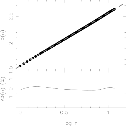
Figure 10: Relation between the function $\Phi(n)$ and the logarithm of the Sersic index (see the text). The grey curve in the upper panel marks the best-fitting line of $\Phi(n)$ vs. $\log n$. The lower panel shows the residuals of the linear fit (solid line).

7.3 The waveband dependence of the PHP

Since the variation of ${<\!\mu\!>_{\rm e}}$  between different wavebands is proportional to the galaxy colour (see Eq.LABEL:magn) and therefore to galaxy luminosity, through the CM relation, the PHP slopes of $\mathrm{MS\,1008}$   in the optical and NIR wavebands can be used to constrain how the ratios $\frac{n_{\rm R}}{n_{\rm K}}$ and $\frac{r_{\rm e,R}}{r_{\rm e,K}}$ vary along the galaxy sequence. In Appendix D, we show that, by using the $R$-band PHP equation and the $R$-$K$ CM relation, it is possible to derive an equation which is analogous to that of the $K$-band PHP, except for a term which is proportional to $\log\frac{n_{\rm R}}{n_{\rm K}}$. It turns out, therefore, that the waveband variation of the PHP does not depend significantly on the ratio of effective radii, but it mainly informs on how the ratio of Sersic indices vary with other structural parameters of galaxies.

As detailed in Appendix D, assuming that the ratio of shape parameters is only a function of the galaxy luminosity, i.e.

$$\log\frac{n_{\rm R}}{n_{\rm K}}=\omega_{1}K+\omega_{2},$$ (10)

where $K$ is the total luminosity in the $K$ band, we obtain two independent constraints on $\omega_{1}$ from the $R$- and $K$- band values of $a$ and $b$ respectively. These constraints are

$$\begin{array}[]{l}\omega_{1}=\frac{a_{\rm R}/a_{\rm K}-1-5b_{\rm R}\Gamma}{5a_{\rm R}},\end{array}$$ (11)

for the coefficient $a$, and

$$\begin{array}[]{l}\omega_{1}=\frac{(b_{\rm K}-b_{\rm R})(1+5b_{\rm R}\Gamma)}{a_{\rm R}(1-5b_{\rm R})},\end{array}$$ (12)

for the coefficient $b$, where $\Gamma$ is the slope of the $R-K$ CM relation of $\mathrm{MS\,1008}$. Using the values of $a$ and $b$ from Table 4 and Table 6, and taking into account the correlation of uncertainties on PHP coefficients, we obtain $\omega_{1}=0.035\pm 0.035$ ($\sim 8\pm 8\%$) and $\omega_{1}=-0.2\pm 0.2$ ($-46\pm 46\%$) from the first and second equations respectively. We note (i) that the two values of $\omega_{1}$ are consistent with each other, showing that the ansatz in Eq. 10 is compatible with the values of the PHP slopes, and (ii) that the first equation sets much stronger constrains on the value of $\omega_{1}$, implying that the variation of $\log\frac{n_{\rm R}}{n_{\rm K}}$ on galaxy luminosity is mainly driven by the $\log n$  coefficient of the PHP. Since the value of $\omega_{1}$ is fully consistent with zero, we conclude that the ratio of optical-NIR shape parameters does not change or can have only a mild variation with galaxy luminosity. This result can be compared with the findings of La Barbera et al. (2003, hereafter LBM03), who showed that the waveband variation of the Kormendy relation slope constrains how the ratio of effective radii between different wavebands vary with galaxy luminosity. In other terms, the waveband dependences of the KR slope and of the PHP $\log n$  slope constrain the variation with luminosity of the ratios of galaxy radii and shape parameters respectively. This is an interesting result, since these ratios fully characterize the radial colour profile in galaxies. Since LBM03 found that $\frac{r_{\rm e,opt}}{r_{\rm e,NIR}}$ does not change significantly with luminosity, the above result indicates that all the properties of the colour profile in galaxies (that is its shape and gradient) do not change with luminosity. The existence of a correlation between the colour profile and galaxy luminosity is a still debated issue. For example, Peletier et al. (1990) found no correlation among the internal colour gradients of field ETGs and their luminosities, while Tamura & Ohta (2003) found that for very bright ETGs in a nearby cluster such correlation could exist. A steepening of colour gradients with galaxy luminosity is a natural expectation of the monolithic collapse model (Larson, 1974) of galaxy formation, since galactic winds blow earlier in less massive galaxies, preventing gas dissipation to carry heavy metals in the center, and producing, therefore, a less steep gradient in these systems. On the other hand, in a hierarchical scenario of galaxy formation, merging would dilute stellar population gradients in larger galaxies (White, 1980), sweeping out or reversing the colour gradient-luminosity relation. The implications deriving from a multiwavelength analysis of the KR and the PHP should be carefully taken into account by any model aimed to explain the processes underlying the formation and evolution of ETGs.

7.4 The redshift dependence of the PHP

Since the PHP is a correlation among global parameters of ETGs which are strictly related both to their luminosity density (${<\!\mu\!>_{\rm e}}$) and internal structure (${r_{\rm e}}$  and $n$), its slopes indicate how these properties vary along the galaxy sequence. The fact that the PHP slopes do not change significantly up to $z\sim 0.3$ implies that in this redshift range (i) the luminosity evolution of (bright) ETGs is not significantly different along the galaxy sequence and (ii) correlations among structural properties and galaxy mass do not change significantly with $z$. Point (i) follows directly from the PHP equation (Eq. 1). If the evolution with $z$ of ${<\!\mu\!>_{\rm e}}$  would depend on ${\log r_{\rm e}}$  and/or $n$, we would expect to find a change of $a$ and $b$ with redshift (see Eq. 1). The fact that the luminosity evolution of (bright) ETGs does not change along the galaxy sequence is consistent with results of Kormendy relation studies at intermediate redshifts (e.g. Barger et al. 1998; Ziegler et al. 1999; La Barbera et al. 2003), which found that the luminosity evolution of ETGs is almost independent of galaxy size. Point (ii) can be analyzed by considering Eq. 8. If the PHP origins from a correlation between specific entropy and galaxy mass, the slopes of the PHP are fully characterized by the slopes of the $M/L$ vs. $M$ and $s$ vs. $M$ relations. Since FP studies seem to indicate that the $M/L$ vs. $M$ relation does not change significantly at $z\sol 0.3$ (Kelson et al. 2000), the result of Section 6.2 implies that the slope of the $s$ vs. $M$ relation does not change significantly with $z$. This is consistent with the idea that merging is the physical process which builds up the $s$–$M$ relation (MLC00) and that bright ETGs in clusters are mostly assembled at redshift $z\sog 1$ (e.g. Kauffmann 1995).

As shown in Section 6.2, the zero-point of the PHP can be applied to constrain the mean luminosity evolution of ETGs with redshift. This use of the PHP is based on the fact that its slopes do not evolve with redshift and that the variations with $z$ of the mean values of both ${\log r_{\rm e}}$  and $\log n$  are known exactly (see Eq. 6). Assuming $\Delta(\overline{\log r_{\rm e}})=0$ and $\Delta(\overline{\log n})=0$, we find that the evolution of the zero-point of the PHP from $z\sim 0.3$ to $z\sim 0$ is consistent with the cosmological dimming of mean surface brightness and the passive fading of an old stellar population with a high formation redshift, $z_{\rm f}>1$–$2$. The hypothesis $\Delta(\overline{\log r_{\rm e}})=0$ is well motivated by the findings of different studies that the distribution of radii of ETGs does not change significantly at intermediate redshifts (La Barbera et al., 2002; Shen et al., 2003). On the other hand, assuming $\Delta(\overline{\log n})=0$ is a more tricky point, since a morphology-density relation is known to exist and this relation evolves with redshift (Dressler et al., 1997). To account for this effect, we calculated the mean values of $\log n$  for the sample of $\mathrm{MS\,1008}$   and that of GRA02. The difference between the two values turned out to be $\Delta(\overline{\log n})=-0.045\pm 0.05$, in agreement with the hypothesis $\Delta(\overline{\log n})=0$.

Due to heavy request for measuring velocity dispersions of distant galaxies, it is clearly of great interest to have shown that the PHP is a valuable tool for measuring the luminosity evolution of ETGs. In the future, it will be very interesting to derive the PHP for samples of galaxies at higher redshift, taking advantage (a) of the relatively small dispersion of the PHP with respect to other purely photometric correlations, and (b) of the fact that the PHP slopes seem not to depend on the waveband, allowing, therefore, a straightforward comparison of the PHP among different redshifts (different restframe bands) to be performed.

8 Summary

Using a unique dataset of optical and NIR data, we have done a detailed study of the Photometric Plane (PHP) relation in the $R$, $I$ and $K$ bands for a large sample of ETGs in the rich galaxy cluster $\mathrm{MS\,1008}$ at intermediate redshift ($z\sim 0.3$). We have derived the PHP by accounting for selection effects and other issues related to the fit of this relation. Our main findings can be summarized as follows.

1. The PHP is indeed a plane in the space of the quantities ${\log r_{\rm e}}$, ${<\!\mu\!>_{\rm e}}$  and $\log n$, i.e., there is no significant departure from a purely flat relation (Section 5.1). We have shown that this result is consistent with the fact that the PHP origins from a systematic variation of specific entropy of ETGs along the galaxy sequence. For isotropic, non rotating, one component models, the specific entropy turns out, in fact, to be almost an exact linear combination of ${\log r_{\rm e}}$, ${<\!\mu\!>_{\rm e}}$  and $\log n$.

2. We have found no waveband dependence of the PHP slopes (Section 6.1). Both the PHP coefficients and its intrinsic scatter are fully consistent among the optical and NIR wavebands.

3. The scatter around the PHP is about $\sim 32$ %, which is larger than the average scatter of the Fundamental Plane, but smaller than that of the Kormendy relation and the photometric or the ‘$\rm Mg_{2}$ Fundamental Plane’ (Section 7.1).

   By comparing the PHP coefficients at $z=0.3$ with those at $z\sim 0$ for the sample of GRA02, we have found that the slopes of the PHP do not show a significant variation in this redshift range. This fact has important consequences on our understanding of the evolution of bright ETGs, as discussed in Section 7.4. Namely:

4. the luminosity evolution does not change significantly along the galaxy sequence;

5. the slope of the relation between specific entropy and galaxy mass does not change since $z\sim 0.3$.

   Both these findings are in agreement with the fact that bright ETGs are already assembled at high redshift. Finally, we have demonstrated that the PHP is a valuable tool for measuring the luminosity evolution of ETGs. We have found that

6. the mean luminosity of ETGs is consistent with the passive fading of an old stellar population, with formation redshift $z_{\rm f}>1$.

Due to the heavy request of telescope time for measuring velocity dispersions, constructing the FP relation for large samples of galaxies at $z>0.5$ becomes impracticable. The present results show that the PHP could be a very interesting alternative tool for the study of ETGs at high redshifts.

Appendix A PSF modeling

The stars in the $R$, $I$, $K(S)$  and $K(I)$  images were fitted by the following formula:

$$\mathrm{PSF(r)=\sum_{k=1}^{p}A_{k}(\theta)\cdot M_{k}(r,\theta),}$$ (13)

where $r$ is the distance to the star center, $\theta$ is the polar angle, $M\propto\left[1+(r/r_{\rm c})^{2}\right]^{-\beta}$ is the Moffat law (Moffat, 1969), $p$ is the number of Moffat functions, and $A$ is an angular modulation function. PSF asymmetries were described by adopting the formula:

$$A(\theta)=\sum_{m=1}^{q}\left[a_{m}\cos(m\cdot\theta)+b_{m}\sin(m\cdot\theta)\right].$$ (14)

The values of $p$ and $q$ were chosen interactively for each image in order to obtain an accurate modeling of stellar isophotes. This was achieved by using two or three Moffat functions, depending on the image, with $q\leq 3$. To account for PSF variations across the frames, each galaxy was fitted by using a local PSF model, obtained from the nearest star in the field. The PSF modeling in the $R$ band image is illustrated in Fig. 11, where we show residuals of star fitting as a function of both the distance to the star center and the polar angle. Residuals are plotted for two fitting cases, with and without the angular modulation function. The figure shows that the adopted models give an accurate description of the PSF, allowing both the radial and the angular behaviour of the PSF to be reproduced. We note that the use of asymmetric terms in the fit allows a better centering of the PSF model to be obtained. Hence the improvement in the radial trend of PSF residuals which is observed in Fig. 11. Similar results were also obtained in the analysis of the images of $\mathrm{MS\,1008}$   in the other bands.

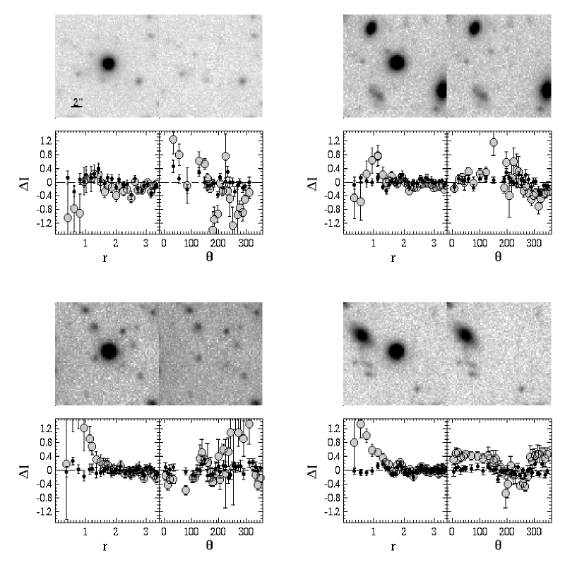
Figure 11: PSF fitting to four stars in the FORS1 $R$-band image. Each plot shows the image of the star (upper-left panel), the residual map (upper-right), and mean fitting residuals in units of the background standard deviation as a function of the radial and angular coordinates (lower-left and lower-right panels, respectively). Large gray symbols and small black circles denote the residuals obtained by respectively excluding and including the angular modulation function in the PSF fit (see text for details). The spatial scale of each image is the same of that shown in the upper–left plot.

Appendix B Uncertainties on ${r_{\rm e}}$, ${<\!\mu\!>_{\rm e}}$  and $n$

Uncertainties on structural parameters were estimated by applying the 2D fitting method to simulated galaxy images. For each galaxy in the $R$, $I$, $K(S)$  and $K(I)$  bands, we used the best-fitting values of ${r_{\rm e}}$, ${<\!\mu\!>_{\rm e}}$  and $n$  to construct a set of seeing–convolved Sersic models to which both photon and read-out noise were added. In order to account for uncertainties due to PSF modeling and to image masking, each simulation was obtained by using a different PSF, according to the uncertainties on the PSF fitting parameters, while the 2D fitting was performed by using the same PSF and the same mask of the real galaxies. For each galaxy, uncertainties on structural parameters were estimated from the covariance matrix of 2D best-fitting parameters for the corresponding set of simulations. The mean uncertainties on ${\log r_{\rm e}}$, ${<\!\mu\!>_{\rm e}}$  and $\log n$  amount to $\sim\!0.03$ dex, $\sim\!0.18$ $\rm mag/arcsec^{2}$ and $\sim\!0.05$ dex respectively, in $R$; to $\sim\!0.05$ dex, $\sim\!0.26$ $\rm mag/arcsec^{2}$ and $\sim\!0.09$ dex in $I$; to $\sim\!0.06$ dex, $\sim\!0.27$ $\rm mag/arcsec^{2}$ and $\sim\!0.06$ dex in $K(I)$; and to $\sim\!0.07$ dex, $\sim\!0.34$ $\rm mag/arcsec^{2}$ and $\sim 0.08$ dex in $K(S)$.

In Fig. 12 we compare the structural parameters of the $N=112$ galaxies in common between the $R$ and $I$ bands. We note that the mean differences of the distributions are fully consistent with zero, in agreement with the fact that $R$ and $I$ bands at $z\sim\!0.3$ sample a very similar spectral region and ETGs have small optical–optical colour gradients. For this reason, the widths of the distributions in Fig. 12 provide a rough estimate of the mean uncertainty on ${\log r_{\rm e}}$, ${<\!\mu\!>_{\rm e}}$  and $\log n$. These values are fully consistent with those obtained by adding in quadrature the above mean uncertainties on structural parameters. In Fig. 13 we compare the structural parameters of the $N=38$ galaxies in common between the $K(S)$  and the $K(I)$  samples. Again, the mean differences of the distributions are fully consistent with zero, showing that no significant systematic effects are present. We also note that the standard deviations shown in Fig. 13 agree with what expected on the basis of the mean errors on structural parameters (see above).

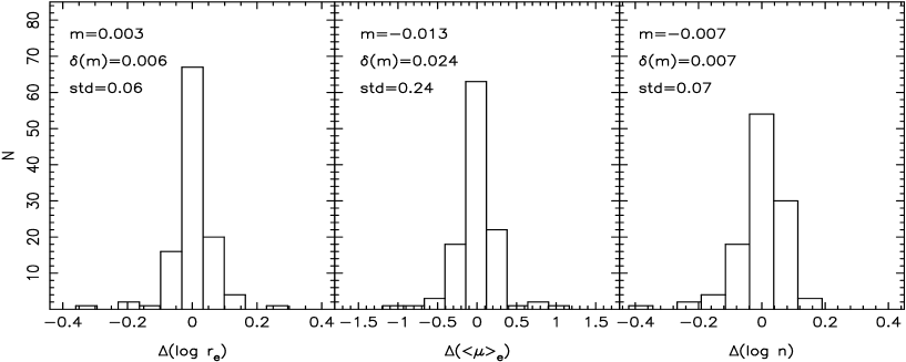
Figure 12: Comparison of structural parameters for the $\rm N=112$ galaxies in common between the $R$- and $I$-band samples. The quantities $m$, $\delta(m)$ and $std$ are the mean value, the uncertainty on the mean, and the standard deviation for each distribution.

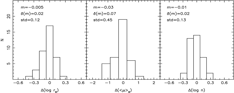
Figure 13: The same of Fig. 12 for the $N=38$ galaxies in common between the $K(S)$  and $K(I)$  samples.

Appendix C Specific entropy of ETGs

As shown by MLC00, the specific entropy of a galaxy, $s$, is given by the following formula:

$$s=M_{\rm T}^{-1}\int\left(\ln P^{3/2}\rho^{-5/2}\right)\rho\,dV,$$ (15)

where $\rho$ and $P$ are the 3D density and pressure fields, respectively, while $M_{\rm T}$ is the total mass. Following LGM99 and MLC00, we consider spherical, non-rotating galaxy models, with negligible radial gradients of the mass-to-light ratio. For such models the function $\rho(r)$ is obtained directly from the 2D Sersic law by solving the Abel integral equation, while $P(r)$ is calculated from the equation of hydrostatic equilibrium, $\frac{d\!P}{d\!r}=-GM\rho/r^{2}$, where the mass profile $M(r)$ is obtained from a direct integration of $\rho(r)$. The functions $\rho(r)$, $M(r)$ and $P(r)$ can be written as products of dimensional factors for dimensionless functions:

$$\rho(r)=M/L\cdot I_{0}/R_{\rm e}\cdot\tilde{\rho}(s)$$ (16)

$$M(r)=M/L\cdot I_{0}\cdot R_{\rm e}^{2}\cdot\tilde{M}(s)$$ (17)

$$P(r)=G(M/L\cdot I_{0})^{2}\cdot\tilde{P}(s)$$ (18)

where $s=r/R_{\rm e}$ is the dimensionless radius and $I_{0}$ is the 2D central surface brightness. By substituting the previous formulae in Eq. 15, and by using the relation between $I_{0}$ and $<\!I\!>_{\rm e}$ (Eq. LABEL:magn), we obtain Eqs. 8 and 9.

Appendix D Optical-NIR PHP

Considering the optical-NIR colour-magnitude relation, $R-K=\Gamma\cdot K+\Delta$, where $R-K$ and $K$ are total galaxy colours and magnitudes, and using the definition of total magnitude (Eq. LABEL:magn), we can write the R-band PHP relation, $\log R_{\rm e,R}=a_{\rm R}\cdot\log n_{\rm R}+b_{\rm R}\cdot<\!\mu\!>_{\rm e,R}+c_{\rm R}$, where the subscript $\rm R$ denotes the waveband, as follows:

$$\begin{array}[]{l}\log\frac{R_{\rm e,R}}{R_{\rm e,K}}+\log R_{\rm e,K}=\\ a_{\rm R}\log\frac{n_{\rm R}}{n_{\rm K}}+a_{\rm R}\log n_{\rm K}+b_{\rm R}\left(<\!\mu\!>_{\rm e,R}-<\!\mu\!>_{\rm e,K}\right)+\\ +b_{\rm R}<\!\mu\!>_{\rm e,K}+c_{\rm R}=\\ =a_{\rm R}\log\frac{n_{\rm R}}{n_{\rm K}}+a_{\rm R}\log n_{\rm K}+b_{\rm R}\left[\Gamma<\!\mu\!>_{\rm e,K}-5\Gamma\log R_{\rm e,K}\right.+\\ \left.-2.5\Gamma\log(2\pi)+\Delta+5\log\frac{R_{\rm e,R}}{R_{\rm e,K}}\right]+b_{\rm R}<\!\mu\!>_{\rm e,K}+c_{\rm R}.\\ \end{array}$$ (19)

From this equation, we obtain:

$$\begin{array}[]{l}\log R_{\rm e,K}=\left(1+5b_{\rm R}\Gamma\right)^{-1}\cdot\left\{a_{\rm R}\log\frac{n_{\rm R}}{n_{\rm K}}+(5b_{\rm R}-1)\log\frac{R_{\rm e,R}}{R_{\rm e,K}}+\right.\\ \left.a_{\rm R}\log n_{\rm K}+b_{\rm R}(1+\Gamma)<\!\mu\!>_{\rm e,K}+\left[c_{\rm R}+b_{\rm R}\Delta-2.5\Gamma\log(2\pi)\right]\right\}.\end{array}$$ (20)

We note that since $(5b_{\rm R}-1)\sim 0$ (see Table 4), the term $\log\frac{R_{\rm e,R}}{R_{\rm e,K}}$ in Eq. 20 can be neglected. Moreover, since $\left(1+5b_{\rm R}\Gamma\right)^{-1}\cdot(1+\Gamma)\sim 1$, we obtain from the previous equation:

$$\begin{array}[]{lll}\log R_{\rm e,K}&\simeq&\left(1+5b_{\rm R}\Gamma\right)^{-1}\cdot a_{\rm R}\log\frac{n_{\rm R}}{n_{\rm K}}+\left(1+5b_{\rm R}\Gamma\right)^{-1}\cdot\\ &&\cdot a_{\rm R}\log n_{\rm K}+b_{\rm R}<\!\mu\!>_{\rm e,K}+const.\end{array}$$ (21)

We note that this equation is similar to that of the PHP in the $K$ band, except for a term which is proportional to the ratio of shape parameters between the $R$ and $K$ bands. Substituting the ansatz of Eq. 10 in the previous equation, we obtain a relation identical to that of NIR PHP. Comparing the slopes of this relation with the values of $a$ and $b$ in the $K$ band, we obtain Eqs. 11 and 12, respectively.

References

- Barger et al. (1998) Barger, A.J., Aragón-Salamanca A., Smail I., Ellis R.S., Couch W.J., Dressler A., Oemler A., Poggianti B.M., Sharples R.M., 1998, ApJ, 501, 522
- Bruzual & Charlot (2003) Bruzual G., Charlot S., 2003, MNRAS, 344, 1000
- Bertin & Arnout (1996) Bertin E., Arnout S., 1996, A&AS, 117, 393
- Busarello et al. (2002) Busarello G., Merluzzi P., La Barbera F., Massarotti M., Capaccioli M., 2002, A&A, 389, 787
- Busarello et al. (1997) Busarello G., Capaccioli M., Capozziello S., Longo G., Puddu E., 1997, A&A, 320, 415
- Caon, Capaccioli & D’Onofrio (1993) Caon N., Capaccioli M., D’Onofrio M., 1993, MNRAS, 265, 1013
- Capaccioli (1989) Capaccioli M., 1989, in: The world of galaxies, eds. H.G. Corwin, L. Bottinelli Springer-Verlag, Berlin, p. 208
- Ciotti & Bertin (1999) Ciotti L., Bertin G., 1999, A&A, 352, 447
- de Propris et al. (1999) de Propris R., Stanford S.A., Eisenhardt P.R., Dickinson M., Elston R., 1999, AJ, 118, 719
- de Carvalho & Djorgovski (1989) de Carvalho R.R., Djorgovski S., 1989, ApJ, 341, 37
- Djorgovski & Davies (1987) Djorgovski S., Davies M., 1987, ApJ, 312, 59
- Dressler et al. (1987) Dressler A., Lynden-Bell D., Burstein D., Davies R.L., Faber S.M., Terlevich R., Wegner G., 1987, ApJ, 313, 42
- Dressler et al. (1997) Dressler, A., Oemler, A.Jr., Couch, W.J., Smail, I., Ellis, R.S., Barger, A., Butcher, H., Poggianti, B.M., Sharples, R.M., 1997, ApJ, 490, 577
- Gioia & Luppino (1994) Gioia I.M., Luppino G.A., 1994, ApJS, 94, 583
- Gioia et al. (1990) Gioia I.M., Maccacaro T., Schild R.E., Wolter A., Stocke J.T., 1990, ApJS, 72, 567
- Graham (2002) Graham A.W., 2002, MNRAS, 334, 859 (GRA02)
- Jørgensen, Franx & Kjærgaard (1996) Jørgensen I., Franx M., Kjærgaard P., 1996, MNRAS, 2809, 167
- Kauffmann (1995) Kauffmann G., 1995, MNRAS, 274, 161
- Kelson et al. (2000) Kelson D.D., Illingworth G.D., van Dokkum P.G., Franx M., 2000, ApJ, 531, 184
- Khosroshahi et al. (2000) Khosroshahi H., Wadadekar Y., Kembhavi A., Mobasher B., 2000, ApJ, 531, L103
- Khosroshahi et al. (2004) Khosroshahi H., Raychaudhury S., Ponman T. J., Miles T. A., Forbes D. A. 2004, MNRAS, 349, 527
- Kormendy (1977) Kormendy J., 1977, ApJ, 218, 333
- La Barbera, Busarello, Capaccioli (2000) La Barbera F., Busarello G., Capaccioli M., 2000, A&A, 362, 851 (LBC00)
- La Barbera et al. (2002) La Barbera F., Busarello G., Merluzzi P., Massarotti M., 2002, ApJ, 571, 790
- La Barbera et al. (2003) La Barbera F., Busarello G., Merluzzi P., Massarotti M., 2003, ApJ, 595, 127 (LBM03)
- La Barbera et al. (2004) La Barbera F., Merluzzi P., Busarello G., Massarotti M., Mercurio A., 2004, A&A, 425, 797 (LMB04)
- Larson (1974) Larson R.B., 1974, MNRAS, 166, 585
- Lewis et al. (1999) Lewis A.D., Ellingson E., Morris S.L., Carlberg R.G., 1999, ApJ, 517, 587
- Lima Neto et al. (1999) Lima Neto G.B., Gerbal D., Márquez I., 1999, MNRAS, 309, 481 (LGM99)
- Márquez et al. (2000) Márquez L., Lima Neto G.B., Capelato H., Durret E., Gerbal D., 2000, A&A, 353, 873 (MLC00)
- Márquez et al. (2001) Márquez L., Lima Neto G.B., Capelato H., Durret E., Lanzoni, B., Gerbal D., 2001, A&A, 379, 767 (MLC01)
- Moffat (1969) Moffat A.F.J., 1969, A&A, 3, 455
- Pahre, Djorgovski & de Carvalho (1998) Pahre M.A., Djorgovski S.G., de Carvalho R.R., 1998, AJ, 116, 1606
- Peletier et al. (1990) Peletier R.F., Davies R.L., Illingworth G.D., Davis L.E., Cawson M., 1990, AJ, 100, 1091
- Prugniel & Simien (1996) Prugniel P., Simien F., 1996, A&A, 309, 749
- Scalo (1986) Scalo M.J., 1986, Fundamentals of Cosmic Physics, 11, 1
- Sersic (1968) Sersic J.L., 1968, Atlas de Galaxias Australes, Observatorio Astronomico, Cordoba
- Shen et al. (2003) Shen S., Mo H.J., White S.D.M., Blanton M.R., Kauffmann G., Voges W., Brinkmann J., Csabai I., 2003, MNRAS, 343, 978
- Tamura & Ohta (2003) Tamura N., Ohta K. 2003, AJ, 126, 596
- Tran et al. (2004) Tran K.H., Franx M., Illingworth G.D., van Dokkum P.G., Kelson D.D., Magee D., 2004, ApJ, 609, 683
- van Dokkum et al. (1998) van Dokkum, P.G., Franx, M., Kelson, D.D., Illingworth, G.D., Fisher, D., and Fabricant, D. 1998, ApJ, 500, 714
- Yee et al. (1998) Yee H.K.C., Ellingson E., Morris S.L., Abraham R.G., Carlberg R.G., 1998, ApJS, 116, 211
- White (1980) White S.D., 1980, MNRAS, 191, 1
- Wuyts et al. (2004) Wuyts S., van Dokkum P.G., Kelson D.D., Franx M., Illingworth G.D., 2004, ApJ, 605, 677
- Ziegler et al. (1999) Ziegler B., Saglia R., Bender R., Belloni P., Greggio L., Seitz S., 1999, A&A, 346, 13