Modeling the Photopolarimetric Variability of AA Tau

Abstract

We present Monte Carlo scattered light models of a warped disk that reproduce the observed photopolarimetric variability of the classical T Tauri star AA Tau. For a system inclination of $75^{\circ}$ and using an analytic description for a warped inner disk, we find that the shape and amplitude of the photopolarimetric variability are reproduced with a warp which occults the star, located at 0.07 au, amplitude 0.016 au, extending over radial and azimuthal ranges $0.0084$ au and $145^{\circ}$. We also show a time sequence of high spatial resolution scattered light images, showing a dark shadow cast by the warp sweeping round the disk. Using a modified smooth particle hydrodynamics code, we find that a stellar dipole magnetic field of strength 5.2 kG, inclined at $30^{\circ}$ to the stellar rotation axis can reproduce the required disk warping to explain AA Tau’s photopolarimetric variability.

1 Introduction

Observationally, pre-main-sequence T Tauri stars may be divided into classical and weak T Tauri stars (Appenzeller & Mundt 1989; Bertout 1989). The classical T Tauri stars (cTTS) exhibit broad H$\alpha$ indicative of on-going accretion, and are surrounded by large dusty disks inferred from their signature infrared excess emission. On the other hand, weak T Tauri stars (wTTS) do not exhibit the strong H$\alpha$ and large IR excesses and these systems may have ceased accreting and have very low mass disks. Both cTTS and wTTS exhibit photometric variability (a defining feature of T Tauri stars, Joy 1945), with wTTS exhibiting periodic and cTTS quasi-periodic variability (Appenzeller & Mundt 1989; Bertout 1989). Hot and cool spots on the stellar surface are believed to be responsible for the variability, with long lived cool spots dominant in wTTS (Hatzes 1995) and short lived hot spots, possibly linked to the accretion process, dominating in cTTS (Kenyon et al. 1994; Bouvier et al. 1993; Eaton,Herbst & Hillenbrand 1995; Choi & Herbst 1996; Herbst et al. 1994). The currently popular magnetospheric accretion model predicts hot spots on the stellar surface (Ghosh & Lamb 1979; Konigl 1991; Shu et al. 1994). In this model a stellar dipole magnetic field threads, truncates, and possibly warps the circumstellar disk. Disk material is accreted onto the star along magnetic field lines forming hot spots or rings on the stellar surface at the magnetic poles (Mhadavi & Kenyon 1998).

The magnetospheric accretion model has been applied to explain the photometric variability in the cTTS system DR Tau (Kenyon et al. 1994). For the edge-on disk around HH 30 IRS, variability has been observed in both HST images (Burrows et al. 1996; Stapelfeldt et al. 1999; Cotera et al. 2001) and ground based $VRI$ photometry (Wood et al. 2000). The variability in HH 30 IRS has been modelled as due to hot spots (Wood & Whitney 1998, Wood et al. 2000) and a disk warp (Stapelfeldt et al. 1999), but no period has so far been determined. Photopolarimetric variability has recently been observed in the cTTS AA Tau (Bouvier et al. 1999, 2003) and has been interpreted as due to occultation of a star by a warp in the inner regions of a circumstellar disk. The variability is found to have a period of 8.2 days, but the variations sometimes turn-off, possibly due to non-steady accretion.

In this paper, we extend our Monte Carlo photopolarimetry simulations of systems with hot star spots (Wood et al. 1996; Wood & Whitney 1998; Stassun & Wood 1999) to include the effects of disk warps. We construct a warped disk model that reproduces the photopolarimetric variability of AA Tau. Then, using a modified SPH code incorporating forces from an inclined dipole stellar magnetic field, we explore the magnetic field strength and configuration required to warp the AA Tau disk and reproduce the observed photopolarimetric variability. § 2 describes the photopolarimetric data. § 3 presents models for the system using the SED to constrain the large scale disk structure, photpolarimetric variability to constrain the warping of the inner disk, and we also present a time sequence of high spatial resolution scattered light images. § 4 presents our SPH simulations of a disk with an inclined stellar dipole field, and we summarise our results in § 5.

2 AA Tau Photopolarimetry

The photopolarimetry of AA Tau has been reported in a number of studies. The young star at the heart of the system has been classified as a K7$V$ (Kenyon & Hartmann 1995), with a mass of $0.8M_{\odot}$, radius of $1.85R_{\odot}$ and an effective temperature of $4030\pm 30$ K (Bouvier et al. 1999). From analysis of the photometric variability the system’s disk, inferred from the IR excess emission (e.g., D’Alessio et al. 1999), is estimated to be at an inclination of $70^{\circ}$ or greater (Bouvier et al. 1999). The observed photometric variability is achromatic and is attributed to occultation of the star by a warp in the inner disk (Terquem & Papaloizou 2000; Bouvier et al. 2003). The occultation results in $\Delta V\sim 1$ mag, has a duration of around 3-4 days, and recurs every 8.2 days, but occasionally an occultation event is missing. Observations show the overall brightness level and depth of eclipses are variable (Bouvier et al. 2003), suggestive of stochastic magnetospheric accretion in AA Tau. Throughout this study the ’time averaged’ photopolarimetric variations given here are used as the basis for the model. Assuming a Keplerian disk, the warp responsible for the periodic occultation must be located at 0.07 au (Bouvier et al. 2003).

Polarimetry studies show that the linear polarisation increases as the observed flux decreases and that the polarisation has a range of $0.6\%-1.3\%$ (Ménard et al. 2003). The polarisation position angle is shown to vary from $0^{\circ}$ to almost $30^{\circ}$ (Bouvier et al. 1999) and studies of nearby stars exhibit similarly large position angle variations. The large position angle variations are attributed to interstellar polarisation of around 0.5%, so the intrinsic polarization is variable in the range $\sim$ $0.1\%-0.8\%$ (Ménard et al. 2003).

3 Radiation Transfer Models

We model AA Tau’s SED and photopolarimetry using our suite of Monte Carlo scattered light and radiative equilibrium codes. For the SED models we use an axisymmetric disk to determine the disk shape and mass. The photopolarimetric modelling uses a non-axisymmetric warped inner disk described below.

As we model the time dependent photopoalrimetry with a warped disk, a fully self-consistent model should calculate the 3D time-dependent disk temperature and density structure and time dependent SED. Such a calculation is beyond the scope of this paper and instead we present three separate models. The first models AA Tau’s SED with an axisymmetric disk. The disk structure is calculated by enforcing vertical hydrostatic equilibrium in the disk as described in Walker et al.(2004). In the second model we model the photopolarimetry using an analytic description for warping of the inner disk and for the outer disk we use the hydrostatic disk structure derived from the SED modelling. We use the height and shape of the warp from these analytic models as a guide for our dynamical models of the interaction of a disk with a dipole stellar magnetic field. We present the resulting photopolarimetry from this model, again using the disk structure derived from SED models for the outer disk.

We do not expect the time dependent 3D disk structure (due to shadowing of different regions of the outer disk by the warp) to effect our simulated photometric variability. The photometric variability is primarily produced by occultations of the star and the contribution from scattered starlight in the outer disk is small. However, the shape of the outer disk may be important for accurately modelling the polarimetric variability because it is produced by the scattering of starlight. We plan to explore three dimensional disk structure models in the future. In the meantime, we proceed with the modelling as outlined above and detailed below.

3.1 Disk Structure from SED Modelling

Table 1: Dust Properties

	$\kappa$ (cm-2g-1)	$a$	$g$	$P$ (%)
$U$	46.2	0.47	0.64	39.3
$B$	42.3	0.48	0.63	41.1
$V$	37.5	0.49	0.62	40.6
$I$	28.9	0.52	0.60	38.1

Figure 1: Spectral energy distribution data and model for AA Tau. The dotted line is the adopted input stellar spectrum and the three solid lines are the model SEDs for inclinations of (from top to bottom) $65^{\circ}$, $68^{\circ}$ and $71^{\circ}$. The different data points at 60 and 100 $\mu$m represent $IRAS$ (squares) and $ISO$ (triangles) observations.

AA Tau’s spectral energy distribution exhibits the large infrared excess emission characteristic of dusty protoplanetary disks. We model the SED with our Monte Carlo radiative equilibrium techniques (Bjorkman & Wood 2001; Wood et al. 2002; Whitney et al. 2003) updated to include an iterative loop to calculate the disk structure for an irradiated steady accretion disk in vertical hydrostatic equilibrium (Walker et al. 2004). This approach follows D’Alessio et al. (1999) in adopting Shakara & Sunyaev (1973) $\alpha$-disk theory to describe cTTS accretion disks. Therefore the disk density is not parameterised by power laws as in our previous SED models (e.g., Wood et al. 2002; Rice et al. 2003). In our simulations we adopt the dust opacity model which we have used to successfully model the SEDs of the HH 30 IRS and GM Aur disks (Wood et al. 2002; Schneider et al. 2003; Rice et al. 2003). The wavelength dependence of this dust opacity is displayed in Wood et al. (2002, Fig. 2) and has $\kappa_{B}/\kappa_{K}=2.5$ which is in the range of “good fits” as determined from the scattered light models of the HH 30 IRS disk using parametric disk models (Watson & Stapelfeldt 2004). The optical dust scattering properties (opacity, $\kappa$, albedo, $a$, phase function asymmetry parameter, $g$, and maximum polarisation, $P$) are shown in Table 1. These parameters are incorporated into our scattered light models as described in Code & Whitney (1995).

Our iterative Monte Carlo radiative equilibrium code self-consistently calculates the disk density and temperature structure and emergent spectrum at a range of viewing angles. From consideration of the photopolarimetric variability, AA Tau’s inclination has been estimated to be around $70^{\circ}$. Our simulations show that we can reproduce the AA Tau SED at a viewing angle of $i\sim 70^{\circ}$ with the following parameters $T_{\star}=4000$ K, $R_{\star}=1.9R_{\odot}$, $R_{d}=150$ au, and $\dot{M}=7.5\times 10^{-9}M_{\odot}{\rm yr}^{-1}$, corresponding to a total disk mass of $M_{d}=0.02M_{\odot}$. The code calculates an inner radius for the disk of $7R_{\star}$, corresponding to our adopted dust destruction temperature of 1600 K.

Figure 1 shows observations of AA Tau and our SED model for the system described above, viewed at $i=65^{\circ}$, $68^{\circ}$ and $71^{\circ}$. Observations come from the Kenyon & Hartmann (1995) compilation (squares) with additional $ISO$ fluxes (triangles) from Chiang et al. (2001). The input stellar spectrum is from a Kurucz model atmosphere (Kurucz 1994). For inclinations $i>70^{\circ}$, the direct optical starlight becomes obscured by the flared disk. Therefore if the system inclination is indeed greater than $70^{\circ}$, this points to some potential shortcomings in our models. For example, some dust settling could effectively reduce the disk scale-height and therefore allow the star to be viewed at inclinations $i>75^{\circ}$ (e.g., Dullemond & Dominik 2004). We have not attempted to fit the optical flux, since that is observed to vary and is the subject of the next section. The point of this SED model is to obtain estimates for the disk mass and density structure based on a physically plausible disk model. We then use this as the outer disk structure in our subsequent optical scattered light models that use a warped inner disk. Future work will investigate the effects of dust settling on the SED and inclination determinations.

3.2 Photopolarimetry Models and Analytic Disk Warping

The observed photopolarimetric variability in AA Tau has been interpreted as eclipses of the star by a warp in the circumstellar disk. To investigate this interpretation, we have constructed scattered light simulations where we introduce a warp into the axisymmetric disk geometry that we derived from SED fitting. Informed by the dynamical model (Section 4), where the disk midplane is not raised and lowered to produce the warp but material ’piles up’ at the corotation radius, we create the disk warp by introducing an azimuthal, $\phi$, dependence of the disk scale-height,

$$z_{0}=z_{w}\exp{-{1\over 2}[(\phi-\phi_{0})/\Delta\phi]^{2}}\exp{-{1\over 2}[(\varpi-\varpi_{0})/\Delta\varpi]^{2}}$$ (1)

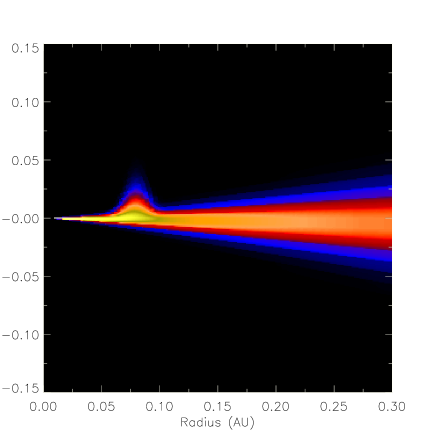
Figure 2: Analytically induced warp used to fit AA Tau’s photopolarimetric variability. The figure shows a slice through the disk density at azimuthal angle $\phi=0^{\circ}$, showing the peak amplitude of the inner disk warp.

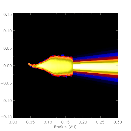
Figure 3: Dynamically induced warp used to fit AA Tau’s photopolarimetric variability. The figure shows a slice through the disk density, showing the peak amplitude of the disk warp.

with $z_{w}$ the amplitude of the warp, $\phi_{0}$ the azimuth of the warp, and $\Delta\phi$ the azimuthal extent of the warp. The warp is further constrained in radius with the second Gaussian function so that it peaks at $\varpi_{0}$ and extends over a radius $\Delta\varpi$. A warp is created in both the positive and negative $z$ directions, with the peaks having a $\pi$ phase separation. A second warp in the negative $z$ direction does not alter our simulated light curves for this viewing angle. Figure 2 shows the warp in the inner regions of the disk on the positive $z$ surface responsible for the photopolarimetric variability. Figure 3 shows the dynamically induced warp in the inner regions of the disk which is of similar dimensions but has a larger radial extent. As mentioned earlier the radial extent of the warp has little effect once it is large enough to fully obscure the central source so this makes no difference to the photopolarimetry of the model.

Figure 4: Photo-polarimetry simulations of a Gaussian shaped warp with an occultation duration of 3.3 days. The upper panel shows the variation in observed flux, with $\Delta m\sim 1$, for U (dotted),B (dashed),V (solid) & I(dot-dashed) bands. The lower panel shows the corresponding linear polarisation with $P=0.4\%-1.05\%$ in the V-band.

Figure 5: Photometry simulations of the dynamically induced warp with an occultation duration of $\sim 3$ days. The upper panel shows the variation in observed flux, with $\Delta m\sim 0.73~{}magnitude$, for U (dotted),B (dashed), V (solid) & I (dot-dashed) bands. The lower panel shows the corresponding linear polarisation with $P=0.6\%-0.8\%$ in the V-band.

After the original interpretation that the variability of AA Tau was due to a warped inner disk (Bouvier et al. 1999), a study by Terquem & Papaloizou (2000) examined the conditions under which an inclined stellar magnetic dipole could reproduce the required warp. They found that a dipole inclined at $30^{\circ}$ is easily capable of inducing a warp of the size proposed by Bouvier et al. (1999). They also discovered that depending on the viscosity of the disk the vertical displacement of the disk varied rapidly (low viscosity) and was likely to cause break up or caused a smoothly varying warp of the kind expected (high viscosity). Both cases would produce variations in light curves that could possibly be distinguished from one another.

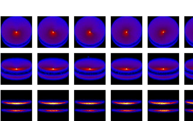
Figure 6: Scattered light images of our warped disk model of AA Tau. The panels on the upper row show the disk at an inclination of $25^{\circ}$, the centre row of panels have inclination $70^{\circ}$ and the panels along the bottom show an inclination of $85^{\circ}$, all are $400$ au on a side. The images cover half a rotation and clearly show the shadowed area caused by the warp occulting the star moving round the disk. To overcome the large dynamic range between starlight and scattered light in the disk, the images are presented on a one-tenth root (square root for the edge on disk) stretch. The faintest regions have a surface brightness of $10^{-6}$ that of the star.

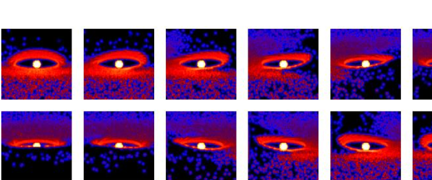
Figure 7: Scattered light images of the warped disk inclined at $75^{\circ}$ and with an image diameter of $0.2~{}au$ clearly showing the material responsible for the photopolarimetric variations occulting the star. To overcome the large dynamic range between starlight and scattered light in the disk, the images are again presented on a one-tenth root stretch. The faintest regions have a surface brightness of $10^{-6}$ that of the star.

Our parameterised inner disk warp simulations that best reproduce the observed photopolarimetry have $i=75^{\circ}$, $z_{w}=0.016$, $\Delta\phi=75^{\circ}$, $\varpi_{0}=0.072$ au and $\Delta\varpi_{0}=0.0084$ au. Figure 4 shows the photpolarimetric light curves for this model. Note that the photometric variability for a warped disk is achromatic, as observed. Even though there is a wavelength dependence to the circumstellar dust opacity, the disk warp is optically thick enough that colour variations in the photometry are not observable. Slight wavelength dependent variations are present in the level of polarisation. In the observed polarimetry of AA Tau (Bouvier et al. 1999) there is a substantial position angle variation of around $0^{\circ}$ to $30^{\circ}$. By comparison with other stars in the vicinity a study by Ménard et al. (2003) attributed this variation to the interstellar medium. After ISM polarisation is removed $\Delta PA$ drops to $0^{\circ}$.In our simulations we find $\Delta PA$ $\sim 4^{\circ}$ indicating that there is in fact some intrinsic $\Delta PA$. If this is the case then it is not unreasonable to assume that the interstellar polarisation is $<0.5\%$. The removal of a smaller interstellar polarisation component would in turn produce a slightly higher linear polarisation value for AA Tau, somewhere between the value stated by Ménard et al. (2003) and Bouvier et al. (1999) mentioned earlier.

Clearly many different warped disk models could match the observations, and we have constrained the parameters as follows:

The direct stellar flux and polarisation from a flared disk are sensitive to the inclination angle (e.g., Whitney & Hartmann 1992). For viewing angles $i>78^{\circ}$, the star becomes blocked by the flared disk and the polarisation increases dramatically (e.g., see Stassun & Wood 1999, Fig. 5) since the relative fraction of scattered to direct starlight increases. For viewing angles $i<70^{\circ}$ we obtain very low polarisation values and would require very large warps, $z_{w}$, to obtain the observed photometric variability. We do not allow warps to exceed $z_{w}/\varpi_{0}=0.3$ in accordance with theoretical models of disk warping (Bouvier et al. 1999). The warp must be constrained to a fairly narrow range in disk radius to obtain the observed variability. Warps extending over large radial distances would not survive due to differential rotation in the disk. The shape of the photopolarimetry light curve allows us to place constraints on the azimuthal extent of the warp. As the occultation itself is reported to last from 3-4 days it implies a warp with an azimuthal extent of $130^{\circ}-175^{\circ}$. The warp in figure 4 matches the observed brightness variation and polarisation of AA Tau. We find that as we increase the warp’s extent around the disk there is very little change in the brightness variation but there is a reduction in the level of polarisation reached during the occultation. Values of $\Delta\phi$ much larger or smaller than what we use result in light curves that show too broad or too narrow an eclipse feature.

For comparison, modelling was carried out using a sinusoidal shaped warp. The duration of the warp was 3.3 days and there was very little change in the photopolarimetry compared to our previous model.For the sinusoidal warp, $\Delta V=1.08$ showing good agreement with the Gaussian model ($\Delta V=1.05$) and the polarisation varied from $0.4\%-1.15\%$ also in good agreement with the Gaussian model where polarisation varied from $0.6\%-1.2\%$.

Finally we modelled the photopolarimetry of the dynamical models magnetically induced warp. A stellar magnetic dipole of 5.2kG inclined at $30^{\circ}$ to the stellar rotation axis produced a warp of approximately the same dimensions as the analytical model. The duration of the occultation event was around 3.3 days with some low level variability lasting slightly longer. The warp produced a variation in photometry, $\Delta V$, of 0.73 Mag. The polarisation was found to vary from $0.3\%-0.6\%$ giving good agreement with the analytical model and the observed variability. Figure 5 shows the photometric light curves for this model at various wavelengths.

In summary we estimate the uncertainty in our models to be $i=75^{\circ}\pm 2^{\circ}$, $\Delta\phi=75^{\circ}\pm 5^{\circ}$, $\Delta\varpi=0.0084\pm 0.0042$ au and $z_{w}=0.016\pm 0.0016$ au.

3.3 Time Sequence Scattered Light Images

In addition to eclipsing the star and producing the observed unresolved photopolarimetric variability, the warp also casts a shadow over the outer regions of the disk. Therefore, a time sequence of high spatial resolution images may detect a shadow sweeping round the disk. Figure 6 shows a sequence of scattered light images at a range of viewing angles for our AA Tau warped disk model. Figure 7 shows a series of ’close-up’ scattered light images of the warp occulting the star at a viewing angle of $75^{\circ}$. These models may be compared with hot star spot models (Wood & Whitney 1998) which show a lighthouse effect of a bright pattern sweeping around the disk. For some warped disk models, the azimuthal extent of the warp may mimic scattered light images due to hot star spots, but multi wavelength photometry can discriminate models: star spots yield chromatic variability, whereas a disk warp yields achromatic photometric variability. Notice that for edge-on viewing the time sequence images for warped disks and disks illuminated by a spotted star (Wood & Whitney 1998) are very similar, and multi-wavelength photopolarimetry is required to break the degeneracy.

For completeness we included in our warped disk models spots of various sizes located at a range of latitudes with a temperature of $8000$ K. We found that a spot with an angular radius of $5^{\circ}$ was more than enough to visibly alter the photometry at all latitudes causing the wavelength dependant effects mentioned above. Therefore a spot covering more than $0.2\%$ of the stars surface area causes a chromatic variation in the photopolarimetry that does not compare with observtions. Figure 8 shows unresolved photopolarimetric models of our warped disk illuminated by a star with hot spots on its surface. The spotted star model exhibits strong colour changes not present in the warped disk model. The shape of both the photometric variation and polarimetric variation curves are also quite different for the spot model purely as a function of the differing geometries involved. These strong colour changes are not reported in AA Tau, however, the HH 30 IRS disk does exhibit a colour dependence (Wood et al. 2000), so it appears that the hot spot models are more appropriate for that system.

Figure 8: Variations in photometry (top panel) and polarisation (bottom panel) for our warped disk illuminated by a spotted star at 4 different passbands, U (dotted), B (dashed), V (solid) & I (dot-dashed). The hot spot is at the same longitude as the warp, a latitude of $65^{\circ}$, has a radius of $5^{\circ}$ and a temperature of $8000$ K. Note the strong wavelength dependence and different shape of the light curve to that generated by a warped disk geometry.

4 Hydrodynamic simulations

Having analytically investigated the size and shape of the inner disk warping required to match AA Tau’s photopolarimetry, we now use a three dimensional hydrodynamics code to explore magnetically induced disk warps. We model the inner accretion disk region of AA Tauri with a three-dimensional smoothed particle hydrodynamics (SPH) code. SPH is a Lagrangian numerical scheme in which gas flow is represented by a system of particles moving with the local fluid velocity (Monaghan, 1992). The SPH method has been applied successfully to accretion disks in a host of astrophysical situations including protoplanetary disks (Rice et al., 2003), cataclysmic variables (Truss et al., 2000) and micro-quasars (Truss & Wynn, 2004) and has been applied to the magnetic warping of disks by Murray et al. (2002). The warping of a disk in response to an offset dipolar field has also been calculated with a three-dimensional Eulerian magnetohydrodynamics code by Romanova et al. (2003).

In our model, we use operator-splitting to solve for the dynamics of the gas flow subject to three forces. The gas pressure force is computed by solving the SPH momentum equation with the standard SPH viscosity term:

$$\frac{d{\bf v}_{i}}{dt}=-\sum_{j}m_{j}\left(\frac{P_{i}}{\rho_{i}^{2}}+\frac{P_{j}}{\rho_{j}^{2}}+\frac{\beta\mu_{ij}^{2}-\alpha\bar{c}_{ij}\mu_{ij}}{\bar{\rho}_{ij}}\right)\nabla_{i}W_{ij}.$$ (2)

Here, $W_{ij}$ is the interpolating kernel between particles i and j, $\bar{c}_{ij}$ is the mean sound speed of the two particles and $\mu_{ij}$ is such that

$$\mu_{ij}=\left\{\begin{array}[]{ll}\frac{H{\bf v}_{ij}\cdot{\bf r}_{ij}}{{\bf r}_{ij}^{2}+0.01h^{2}}&\mbox{${\bf v}_{ij}\cdot{\bf r}_{ij}\leq 0$}\\ 0&\mbox{${\bf v}_{ij}\cdot{\bf r}_{ij}>0$}\end{array}\right.$$ (3)

where $h$ is the smoothing length and $H$ is the local scale height of the disk. The viscosity parameter $\alpha$, should not be confused with the Shakura-Sunyaev viscosity parameter, although Murray (1996) has shown that in three dimensions with $\beta$=0, the net Shakura-Sunyaev viscosity introduced by this model is

$$\alpha=\frac{1}{10}\alpha_{\mathrm{SPH}}.$$ (4)

The gravitational attraction of the star is computed via a simple Runge-Kutta fourth order integrator. We do not consider the self-gravity of the accretion disk, as we are modelling only a small, low-mass region near the central star. Full MHD is not yet possible with SPH, so a third force is added, representing the drag on each particle due to a magnetic dipole field anchored on the star. The dipole field is assumed to co-rotate with the star, but is offset slightly with the rotational axis.

Figure 9: The radial dependence of the magnitude of the magnetic drag acceleration term, plotted here for a surface density profile $\Sigma\sim\rho H\propto 1/r$. In the simulations, the surface density is calculated self-consistently, but in practise departures from this profile are small. The net drag force is directed toward the central star inside the co-rotation radius and its magnitude increases sharply towards the star. Outside the co-rotation radius, the net drag force is weaker and is directed away from the central star. The drag force is zero at $R=R_{\mathrm{co}}$.

The magnetic drag force model has been described by Wynn, King & Horne (1997), and was first included in a SPH scheme by Murray et al. (2002) to investigate the magnetic warping of disks in cataclysmic variables. The model has been developed further in a recent paper by Matthews, Speith & Wynn (2004), in which it is used in a one-dimensional model of accretion disks in T Tauri stars. Here, we incorporate these developments into a fully three-dimensional hydrodynamic study of a circumstellar disk. In the model, the magnetic tension force appears as

$$a_{\mathrm{mag}}\sim\frac{B_{\mathrm{z}}^{2}}{4\pi\rho r_{\mathrm{c}}}\left(\frac{\Omega-\Omega_{*}}{\Omega}\right),$$ (5)

where $\Omega$ and $\Omega_{*}$ are the angular velocities of the gas and the star respectively and $r_{\mathrm{c}}$ is the local radius of curvature of the magnetic field lines. This is approximated as a fraction of the local scale height of the disk,

$$r_{\mathrm{c}}=\zeta H$$ (6)

where $\zeta\leq 1$ (Pearson, Wynn & King, 1997).

For a dipole of magnetic moment $\mu$ we have

$$B_{\mathrm{z}}=\frac{\mu}{r^{3}}.$$ (7)

The drag force acts in a direction perpendicular to the relative velocity of the gas and the rotating field. It is positive, propelling material away from the star, for all radii $r>R_{\mathrm{co}}$, where $R_{\mathrm{co}}$ is the co-rotation radius. Conversely, gas at radii $r<R_{\mathrm{co}}$ feels a net force towards the star. The functional form of this force term is plotted in Figure 9. For numerical convenience, we only model the flow of gas outside a radius $R_{\mathrm{min}}=4R_{*}$, since close to the star the magnetic drag force becomes very large. This has no impact whatsoever on the resolution of structure in the accretion disk itself, which is truncated well outside this radius.

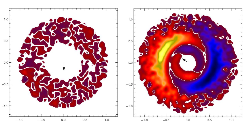
Figure 10: These images of the accretion disk viewed from directly above the star are coloured according to the mean height from the mid-plane at the beginning (left) and end (right) of the simulation. Blue regions are, on average, below the mid-plane while yellow and orange are, on average, above the mid-plane. Regions that remain coplanar with the stellar equator are left white. The initial conditions (left) are chosen such that the altitude of gas at each radius is symmetric about the mid-plane, hence the mean height appears random (but is very close to zero). The axes are scaled in units of $20R_{*}$. Gas that appears inside the co-rotation radius (which lies near 0.45 in these units) is threaded onto the magnetic field lines of the stellar dipole field. The black arrows at the centre of the disk show the projected direction of the north pole of the dipole, which is offset at an angle $30^{\,\circ}$ to the vertical.

We set up an initial disk comprising 500000 SPH particles, extending from the corotation radius $R_{\mathrm{co}}=8.7R_{*}$ to $20R_{*}$, where the stellar radius is taken to be $R_{*}=1.3\times 10^{11}{\mathrm{cm}}$. The midplane of the initial disk is coplanar with the stellar equator and has a surface density profile $\Sigma(r)\propto r^{-1}$. It is flared, with a hydrostatic vertical density profile $\rho(z)=\rho(0)\,{\rm exp}(-z^{2}/2H^{2})$, where $\rho(0)$ is the density in the mid-plane and $H$ is the scale height $c_{\mathrm{s}}/\Omega$. The particles are given radial velocities such that throughout the disk the mass accretion rate is constant at a value $\dot{M}=7.5\times 10^{-9}M_{\odot}{\rm yr}^{-1}$.Here, we are considering the case of a constant mass accretion rate into the inner regions of the accretion disk. Naturally, it is quite possible to surmise that any variations in mass transfer rate will impact on the size and nature of the warping of the disk. This scenario is discussed in a recent paper by Pfeiffer & Lai (2004). We comment that another factor that may affect the long-term behaviour of any warp is magnetic diffusivity, which we do not consider here. It seems likely that a finite resistivity will modify the field structure somewhat, although the importance of this effect for the long-term stability of a disk warp remains unclear.

We use a Shakura-Sunyaev viscosity parameter $\alpha=0.01$, $\beta=0$ and a dipole moment $\mu=1.2\times 10^{37}\,{\mathrm{Gcm^{3}}}$. With $\zeta=1$, this corresponds to a stellar field strength $B(R_{*})=5.2{\mathrm{kG}}$, which is slightly larger than the values usually quoted for T-Tauri stars, in the range $2-3{\mathrm{kG}}$. This field was required to produce the warp described below for the parameters given, although it should be stressed that there is nothing to prevent $\zeta<1$, in which case there is better agreement with the observed field strengths. The magnetic dipole is offset at angle $\pi/6$ to the axis of stellar rotation.

After several orbits under the influence of the magnetic field, a stable warped structure develops near the corotation radius. Figure 10 shows the local average height of the disk above the mid-plane, in the initial and final states. The warp has a maximum vertical height of $\sim 2R_{*}$. This result is consistent with the earlier analysis of Terquem & Papaloizou (2000), who computed the steady warped structure of the disk in AA Tauri, and predicted a similar trailing spiral structure near the corotation radius. We also made a limited study of the effects of changing the tilt angle of the magnetic dipole. Increasing the tilt angle to $5\pi/18$ had little or no effect on the size of the warp, and the resultant disk structure was indistinguishable from that obtained in the original simulation.

5 Summary

We have modelled the photopolarimetric variations of the classical T Tauri system AA Tau. Our results show that a magnetospherically induced warp of the accretion disk at roughly the stellar corotation radius occults the star and reproduces the observed variability. Our SED modelling provides us with estimates of the disk mass and large scale density structure that are subsequently used in our non-axisymmetric scattered light disk models. Spotted star models exhibit a strong wavelength dependence which is not observed in the AA Tau system. Our warped disk model shows no wavelength dependence and can reproduce the occultation period and duration with the required brightness and polarisation variations. A feature of the warped disk model is that it produces a shadow that sweeps around the outer disk and this may be detectable with high spatial resolution time sequence imaging.

Using a modified SPH code, we find that a stellar magnetic dipole of 5.2kG inclined at $30^{\circ}$ to the stellar rotation axis may reproduce the required warp amplitude to occult the star and reproduce the brightness variations. The models we have presented are strictly periodic, so do not reproduce the stochastic nature of AA Tau’s lightcurve (Bouvier et al. 2003). However, our models do show that disk warping resulting from the interaction of the stellar magnetic field with the disk can reproduce the amplitude and shape of the occultation events. In the near future, accurate measurements of the magnetic field structures of T Tauri stars will be possible using Zeeman Doppler Imaging (Petit et al. 2004), allowing more realistic (i.e., non-dipolar) modelling of the stellar magnetic field, its impact on the disk, and observational signatures.

We acknowledge financial support from PPARC studentships (MO, CW, OM), a Postdoctoral Fellowship (MRT), and an Advanced Fellowship (KW).

References

- Appenzeller & Mundt (1989) Appenzeller, I. & Mundt, R., 1989, A&ARv., 1, 291
- Bertout (1989) Bertout, C., 1989, ARA&A, 27, 351
- Bjorkman & Wood (2001) Bjorkman, J.E., & Wood, K., 2001, ApJ, 554 , 615
- Bouvier et al. (1999) Bouvier, J., Chelli, A., Allain, S., Carrasco, L., Costero, R., Cruz-Gonzalez, I., Dougados, C., Fernández, M., Martín, E.L., Ménard, F., Mennessier, C., Mujica, R., Recillas, E., Salas, L., Schmidt, G., & Wichmann, R., 1999, A&A, 349, 619
- Bouvier et al. (2003) Bouvier, J., Grankin, K.N., Alencar, S.H.P., Dougados, C., Fernández, M., Basri, G., Batalha, C., Guenther, E., Ibrahimov, M.A., Magakian, T.Y., Melinkov, S.Y., Petrov, P.P., Rud, M.V., & Zapatero Osorio, M.R., 2003, A&A, 409, 169
- Bouvier et al. (1993) Bouvier, J., Cabrit, S., Fernandez, M., Martin, E.L. & Matthews, J.M., 1993, A&A, 61, 737
- Chiang et al. (2001) Chiang, E.I., Joung, M.K., Creech-Eakman, M.J., Qi, C., Kessler, J.E., Blake, G.A., & van Dishoeck, E.F., 2001, ApJ, 547, 1077
- Choi & Herbst (1996) Choi, P.I. & Herbst, W., 1996, AJ, 111, 283
- Code & Whitney (1995) Code, A.D., & Whitney, B.A., 1995, ApJ, 441, 400
- D’Alessio et al. (1999) D’Alessio, P., Calvet, N., Hartmann, L., Lizano, S., & Canto, J., 1999, ApJ, 527, 893
- Eaton, Herbst & Hillenbrand (1995) Eaton, N.L., Herbst, W. & Hillenbrand, L.A., 1995, AJ, 110, 1735
- Hatzes (1995) Hatzes,A.P., 1995, ApJ, 451, 784
- Herbst et al. (1994) Herbst, W., Herbst, D.K., Grossman, E.J. & Weinstein, D., 1994, AJ, 108, 1906
- Joy (1945) Joy, A., 1945,ApJ, 102, 168
- Kenyon et al. (1994) Kenyon, S.J., Hartmann, L., Hewett, R., Carrasco, L., Cruz-Gonzalez, I., Recills, E., Salas, L., Serrano, A., Strom, K.M., Strom, S.E., Newton, G., 1994, AJ, 107, 2153
- Kenyon & Hartmann (1995) Kenyon, S.J., Hartmann, L., 1995, ApJS, 101,117
- Kurucz (1994) Kurucz, R.L., 1995, CD-ROM 19, Solar Model Abundance Model Atmospheres (Cambridge: SAO)
- Matthews, Speith & Wynn (2004) Matthews O.M., Speith R., Wynn G.A., 2004, MNRAS, 347, 873
- Monaghan (1992) Monaghan J.J., 1992, ARA&A, 30, 543
- Menard et al. (2003) Ménard, F., Bouvier, J., Dougados, C., Melnikov, S.Y., & Grankin, K.N., 2003, A&A, 409, 163
- Murray (1996) Murray J.R., 1996, MNRAS, 279, 402
- Murray et al. (2002) Murray J.R., Chakrabarty D., Wynn G.A., Kramer L., 2002, MNRAS, 335, 247
- Pearson, Wynn & King (1997) Pearson K.J., Wynn G.A., King A.R., 1997, MNRAS, 288, 421
- Petit et al. (2004) Petit, P., Donati, J.-F., & the ESPaDOnS project team, 2004, EAS Publication Series, 9,97
- Pfeiffer & Lai (2004) Pfeiffer H.P., Lai D, 2004, ApJ, 604, 766
- Rice et al. (2003) Rice W.K.M., Wood, K., Armitage P.J., Whitney B.A., Bjorkman J.E., 2003, MNRAS, 339, 1025
- Romanova et al. (2003) Romanova M.M., Ustyugova G.V., Koldoba A.V., Wick J.V., Lovelace R.V.E., 2003, ApJ, 595, 1009
- Schneider et al. (2003) Schneider, G., Wood, K., Silverstone, M., Hines, D.C., Koerner, D.W., Whitney, B., Bjorkman, J.E., Lowrance P.J., 2003, AJ, 125, 1467
- Stassun & Wood (1999) Stassun, K., & Wood, K., 1999, ApJ, 510, 892
- Terquem & Papaloizou (2000) Terquem C., Papaloizou J.C.B., 2000, A&A, 360, 1031
- Truss & Wynn (2004) Truss M.R., Wynn G.A., 2004, in prep.
- Truss et al. (2000) Truss M.R., Murray J.R., Wynn G.A., Edgar R.G., 2000, MNRAS, 319, 467
- Walker et al. (2004) Walker, C., Wood, K., Lada, C.J., Robitaille, T., Bjorkman, J.E., & Whitney B.A., 2004, MNRAS, 351, 607
- Watson & Stapelfeldt (2004) Watson, A.M., & Stapelfeldt, K.R., 2004, ApJ, 602, 860
- Whitney et al. (2003) Whitney, B.A., Wood, K., Bjorkman, J.E., & Cohen, M., 2003, ApJ, 598, 1079
- Wood et al. (1996) Wood, K., Kenyon, S.J., Whitney, B.A., & Bjorkmann, J.E., 1996, ApJ, 458, L79
- Wood & Whitney (1998) Wood, K., & Whitney, B.A., 1998, ApJ, 506, L43
- Wood et al. (2002) Wood, K., Lada, C.J., Bjorkman, J.E., Kenyon, S.J., Whitney, B.A., & Wolff, M.J., 2002, ApJ, 567, 1183
- Wood et al. (2000) Wood, K., Stanek, K.Z., Wolk, S., Whitney, B., Stassun, K., 2000, AAS, 32, 1414
- Wynn, King & Horne (1997) Wynn G.A., King A.R., Horne K.D., 1997, MNRAS, 286, 436