Comparison of map-making algorithms for CMB experiments

We have compared the cosmic microwave background (CMB) temperature anisotropy maps made from one-year time ordered data (TOD) streams that simulated observations of the originally planned 100 GHz Planck Low Frequency Instrument (LFI). The maps were made with three different codes. Two of these, ROMA and MapCUMBA, were implementations of maximum-likelihood (ML) map-making, whereas the third was an implementation of the destriping algorithm. The purpose of this paper is to compare these two methods, ML and destriping, in terms of the maps they produce and the angular power spectrum estimates derived from these maps. The difference in the maps produced by the two ML codes was found to be negligible. As expected, ML was found to produce maps with lower residual noise than destriping. In addition to residual noise, the maps also contain an error which is due to the effect of subpixel structure in the signal on the map-making method. This error is larger for ML than for destriping. If this error is not corrected a bias will be introduced in the power spectrum estimates. This study is related to Planck activities.

1 Introduction

Map-making from an observed time ordered data (TOD) stream is an important step in the data processing pipeline of a cosmic microwave background (CMB) experiment. A number of map-making algorithms which, under the assumption of Gaussian distributed and stationary noise, aim at finding the optimal minimum variance map have been proposed (Wright Wri96 (1996); Borrill Bor99 (1999); Doré et al. Dor01 (2001); Natoli et al. Nat01 (2001)). The destriping technique (Burigana et al. Bur97 (1997); Delabrouille Del98 (1998); Maino et al. Mai99 (1999), Mai02 (2002); Revenu et al. 2000a , 2000b ; Keihänen et al. Kei04 (2004)) is a simpler map-making method.

For this study we utilized simulated one-year TOD streams, that had been produced in the course of the work of the CTP ($C_{\ell}$ for Temperature and Polarisation) Working Group of the Planck Consortia. These TODs represent the output of a single detector of the originally planned 100 GHz LFI (Low Frequency Instrument) channel of the Planck satellite. This simulated data contains contributions from CMB and foreground emissions, as well as from the instrumental noise. The noise was assumed Gaussian distributed and stationary over the entire mission, containing a $1/f$ and a white noise component. We considered temperature anisotropies only; no polarisation.

Output maps were generated from the TODs using three distinct map-making codes. The output maps and their angular power spectra were critically compared. The map-making codes were ROMA (Roma Optimal Mapmaking Algorithm; Natoli et al. Nat01 (2001); de Gasperis et al. deG05 (2005)), MapCUMBA (originally introduced by Doré et al. Dor01 (2001), current version based on the preconditioned conjugate gradient method) and destriping (Keihänen et al. Kei04 (2004)). All methods have been developed to treat Planck-like data.

A minimum variance map maximizes the likelihood function involving the full noise covariance. The ROMA and MapCUMBA algorithms aim at producing the minimum variance map. To accomplish this, the algorithms require knowledge on the characteristics of the instrument noise. Both iterative (Doré et al. Dor01 (2001)) and non-iterative (Natoli et al. Nat02 (2002)) methods to estimate the noise properties directly from the data have been proposed. In this paper ROMA and MapCUMBA are referred to with a common name maximum likelihood (ML) map-making.

Destriping does not employ the noise covariance matrix and does not aim at producing a minimum variance map in this sense. Thus it does not require prior knowledge on the characteristics of the instrument noise. This simplifies the algorithm considerably as compared to the ML map-making. In spite of this, destriping is able to provide an estimate of the low-frequency part of the instrument noise and to return a TOD where these noise components have been removed. Destriping can also be applied to estimate various systematic effects and drifts, remove them and return a cleaned TOD (see e.g. Mennella et al. Men02 (2002)).

The aim of this paper is to compare these two methods, ML (ROMA and MapCUMBA) and destriping, in terms of the maps they produce and the angular power spectrum ($C_{\ell}$) estimates derived from these maps.

This paper is organized as follows. In Sect. 2 we describe the map-making and power spectrum estimation methods applied in this study. The simulated one-year TOD streams are introduced in Sect. 3. The output maps are compared in Sect. 4 and the power spectrum estimates produced from the simulated TODs are examined in Sect. 5. The conclusions are given in Sect. 6. In Appendix A we describe how the output map is split in the (wanted) binned noiseless map and in the (unwanted) reconstruction error map. These quantities were considered in the comparison of the output maps in Sect. 4. In Appendix B we discuss some details about how the $C_{\ell}$ of the maps are related to the input $C_{\ell}$ used to generate the TODs.

2 Methods

Let us denote by a column vector ${\mathbf{y}}$ the samples of the observed TOD. The length of ${\mathbf{y}}$ is $N_{t}$, the number of samples in the total mission. In the map-making problem we assume that the signal samples are scanned from a pixelized temperature map (${\mathbf{m}}$). (This assumption of course represents an approximation to reality, and thus contributes to error in the final maps.) The length of the column vector ${\mathbf{m}}$ is $N_{\rm pix}$, the number of pixels in the map.

The scanning is implemented by a pointing matrix $\mathbf{P}$. The size of the pointing matrix is $[P]=(N_{t},N_{\rm pix})$. Each row contains zeros except for one element with value one, indicating the pixel at which the detector beam centre was pointing when the sample was measured. The map-making methods discussed here utilize pointing information only to the accuracy given by the pixel size. If the instrument beam response is spherically symmetric (and as we are neglecting polarisation), information about the rotation angle of the detector around the line of sight is not needed, and such a simple pointing matrix is sufficient. The pixel temperature of the output map will then represent a convolution of the sky and the beam. We have used in this study simulated TODs corresponding to both spherically symmetric and elliptic beams; but a study of the effects of beam shape is postponed to a future detailed study by the CTP group.

For an asymmetric beam every pixel will be smoothed with a different response that is the mean of the beam orientations of the observations falling in that pixel. Recently a deconvolution map-making algorithm was introduced that can provide an output map where the smoothing of the instrument beam (symmetric or asymmetric) is deconvolved leading to a map that is an estimate of the true sky (Armitage & Wandelt Arm04 (2004)). Deconvolution map-making is beyond the scope of this study.

2.1 ROMA and MapCUMBA

The output map (${\mathbf{m}}$) is solved by minimizing the log-likelihood formula (Natoli et al. Nat01 (2001))

$$\chi^{2}=({\mathbf{y}}-\mathbf{P}{\mathbf{m}})^{T}\mathbf{N}^{-1}({\mathbf{y}}-\mathbf{P}{\mathbf{m}}).$$ (1)

Here $\mathbf{N}$ is the noise covariance matrix $\mathbf{N}=\langle{\mathbf{n}}{\mathbf{n}}^{T}\rangle$, where ${\mathbf{n}}$ is the instrument noise component of the TOD and $\langle\cdot\rangle$ denotes expectation value. A set of linear equations is obtained for the output map

$$\mathbf{P}^{T}\mathbf{N}^{-1}\mathbf{P}{\mathbf{m}}=\mathbf{P}^{T}\mathbf{N}^{-1}{\mathbf{y}}.$$ (2)

Eq. (2) is a general result for the minimum variance map.

Usually ML map-making assumes the noise to be stationary throughout the mission. It is further assumed that the elements of the covariance matrix ($N_{ij}$) vanish when $|i-j|$ is larger than some $N_{\eta}$ and $N_{\eta}\ll N_{t}$. This means that the correlation is significant only across a number of samples that is a tiny fraction of the total length of the TOD. Thus the noise correlation matrix $\mathbf{N}$ can be approximated by a circulant matrix (Natoli et al. Nat01 (2001)). Note that the matrix $\mathbf{N}^{-1}$ is approximately circulant as well. The multiplication $\mathbf{N}^{-1}{\mathbf{y}}$ can be carried out more easily in the frequency domain where $\mathbf{N}^{-1}$ is diagonal (Natoli et al. Nat01 (2001)). Both in the ROMA and in the MapCUMBA algorithms the output map is solved from Eq. (2) with an iterative preconditioned conjugate gradient method. The iterations are repeated until the fractional difference has reached a low enough value (Natoli et al. Nat01 (2001)). This limit is typically on the order of $10^{-6}$.

Due to the circulant matrix approximation each row of the matrix $\mathbf{N}^{-1}$ contains the same element values with a different cyclic permutation. It is assumed that only the elements of a row with $|i-j|\leq N_{\xi}$ ($N_{\xi}\ll N_{t}$) have non-zero values. The rest of the elements are zero. The collection of the non-zero elements (of a row) is called the noise filter. The lag of an element is the difference of its indices ($i-j$). The choice of the value $N_{\xi}$ is a significant decision for the quality of the output maps and for the computation time of the algorithm (Natoli et al. Nat01 (2001)).

Natoli et al. (Nat01 (2001)) have shown how ML map-making can be applied when the instrument noise is only piece-wise stationary.

2.2 Destriping technique

The destriping technique for map-making has been derived from the COBRAS/SAMBA Phase-A study (Bersanelli et al. Ber96 (1996)). It has been implemented by several groups (Burigana et al. Bur97 (1997); Delabrouille Del98 (1998); Maino et al. Mai99 (1999), Mai02 (2002); Revenu et al. 2000a , 2000b ; Keihänen et al. Kei04 (2004); Efstathiou Efs05 (2005)). The implementation studied in this paper (Keihänen et al. Kei04 (2004)) makes use of the fact that Planck is a spinning spacecraft. Detector beams are drawing almost great circles on the sky. Each scan circle is observed several times before the spin axis is repointed. In order to reduce the level of instrumental noise, the signal can be averaged (“coadded”) over these scan circles. In the following we call this averaged scan circle a ring. This coadding shortens the TOD by a factor given by the number of circles between repointings.

Janssen et al. (Jan96 (1996)) has pointed out that the effect of the instrumental noise, in particular $1/f$ noise, on the ring can be approximated by a uniform offset or “baseline”. The key problem in destriping is to find the amplitudes of these baselines. The destriping technique uses the redundancy of the observing strategy by considering the intersections (crossing points) between the scan circles to obtain these amplitudes. A crossing point is defined as two samples from different rings falling on the same pixel. According to this definition, two closely spaced rings may have a crossing point (or a sequence of them, when the rings run parallel) without actually crossing each other, if the distance between the rings is smaller than the pixel size.

The correlated noise component of the TOD is modelled as ${\mathbf{n}}_{\rm{corr}}=\mathbf{F}{\mathbf{a}}$ (Keihänen et al. Kei04 (2004)). Here vector ${\mathbf{a}}$ contains the amplitudes of the baselines and matrix $\mathbf{F}$ unfolds them into a TOD. That is, $\mathbf{F}{\mathbf{a}}$ is a piecewise constant TOD, where the constants are given by the elements of ${\mathbf{a}}$. Once the amplitudes have been solved, $\mathbf{F}{\mathbf{a}}$ is subtracted from the original TOD to produce a cleaned TOD. Finally the output map is binned from the cleaned TOD. This procedure is formally described by minimizing the following likelihood function with respect to the output map ${\mathbf{m}}$ and the amplitudes ${\mathbf{a}}$ (Keihänen et al. Kei04 (2004))

$$\chi^{2}=({\mathbf{y}}-\mathbf{P}{\mathbf{m}}-\mathbf{F}{\mathbf{a}})^{T}({\mathbf{y}}-\mathbf{P}{\mathbf{m}}-\mathbf{F}{\mathbf{a}})/\sigma^{2}.$$ (3)

It is assumed here that the variance ($\sigma^{2}$) of the non-correlated component of the noise is constant throughout the TOD. The amplitudes (${\mathbf{a}}$) can be solved from the equation

$$\mathbf{F}^{T}\mathbf{Z}\mathbf{F}{\mathbf{a}}=\mathbf{F}^{T}\mathbf{Z}{\mathbf{y}}$$ (4)

and the output map is given by

$${\mathbf{m}}=(\mathbf{P}^{T}\mathbf{P})^{-1}\mathbf{P}^{T}({\mathbf{y}}-\mathbf{F}{\mathbf{a}}).$$ (5)

In Eq. (4) $\mathbf{Z}\equiv\mathbf{I}_{t}-\mathbf{P}(\mathbf{P}^{T}\mathbf{P})^{-1}\mathbf{P}^{T}$, where $\mathbf{I}_{t}$ is a unit matrix with dimension $N_{t}$. The matrix $\mathbf{Z}$ is determined by the crossing points of the scan circles. When $\mathbf{Z}$ is acting on the TOD it subtracts from each sample the average of the samples hitting the same pixel.

It turns out that the matrix $\mathbf{F}^{T}\mathbf{Z}\mathbf{F}$ is singular and additional conditions are required before the amplitudes can be solved from Eq. (4). To accomplish this, we require that the sum of the baseline amplitudes is zero.

The destriping method, as given by Eqs. (4) and (5) requires no knowledge of the noise power spectrum. (If it is known that $\sigma^{2}$ varies between different parts of the TOD, this information can of course be incorporated to improve the accuracy of the method.)

The dimension of the matrix $\mathbf{F}^{T}\mathbf{Z}\mathbf{F}$ equals the number of the fitted baselines. A typical number of baselines for a one year TOD (number of rings) is of the order of several thousands. This is a less complex problem than solving the map in the ML method (cf. Eq. (2)), because the number of pixels in the output map is typically between $10^{6}\ldots 10^{8}$.

Generalized approaches to destriping method have been implemented (but not used in the present study) which are able to fit different sets of base functions (in addition to the uniform baseline) and may better remove the contributions of different systematic effects from the TODs (Delabrouille Del98 (1998); Maino et al. Mai02 (2002); Keihänen et al. Kei04 (2004), Kei05 (2005)).

2.3 Estimation of the angular power spectrum

We studied the CMB angular power spectrum estimates obtained from the output maps. For the power spectrum estimation we used the MASTER approach (Monte carlo Apodised Spherical Transform EstimatoR) described by Hivon et al. (Hiv02 (2002)). MASTER has been adapted to operate both with ROMA (Balbi et al. Bal02 (2002)) and with destriping (Poutanen et al. Pou04 (2004)).

The angular power spectrum of the CMB sky $C_{\ell}^{\rm{in}}$ is derived from the spherical harmonic expansion coefficients ($a_{\ell m}$) of the sky

$$C_{\ell}^{\rm{in}}=\frac{1}{2\ell+1}\sum_{m=-\ell}^{\ell}{|a_{\ell m}|^{2}}.$$ (6)

The simulated TODs are generated from such a spectrum, supposed to represent the “real sky”. We call it the input spectrum for our simulation + map-making problem. The $a_{\ell m}$ coefficients are a realisation of the underlying “theoretical” angular power spectrum $C_{\ell}^{\rm{th}}$. The ensemble mean (of many realisations) equals the theoretical spectrum, $\langle C_{\ell}^{\rm{in}}\rangle=C_{\ell}^{\rm{th}}$. The angular power spectrum (pseudo spectrum) of an output map is denoted $\widetilde{C}_{\ell}$. We further define $C_{\ell}^{\rm B}$, which is the angular power spectrum of the binned noiseless map. That map is obtained by binning the samples of the noiseless signal-only TOD to map pixels.

The ensemble mean of the CMB pseudo spectrum depends on the ensemble mean of the spectrum of the sky. Hivon et al. Hiv02 (2002) express this relation as

$$\langle\widetilde{C}_{\ell}\rangle=\sum_{\ell^{\prime}}M_{\ell\ell^{\prime}}F_{\ell^{\prime}}B^{2}_{\ell^{\prime}}D^{2}_{\ell^{\prime}}\langle C_{\ell^{\prime}}^{\rm{in}}\rangle+\langle\widetilde{N}_{\ell}\rangle.$$ (7)

The matrix $M_{\ell\ell^{\prime}}$ is the mode coupling matrix (kernel matrix) determined by the applied sky cut (Hivon et al. Hiv02 (2002)). A symmetric instrument beam is assumed and its smoothing is modelled by $B_{\ell}^{2}$. Pixelisation introduces additional smoothing, which is represented by the pixel window factor $D_{\ell}^{2}$. The filter function $F_{\ell}$ represents a possible distorting effect of map-making and the noise bias $\langle\widetilde{N}_{\ell}\rangle$ the remaining noise.

There are a number of complications in the relation between the spectrum of the output map $\widetilde{C}_{\ell}$ and that of the sky $C_{\ell^{\prime}}^{\rm{in}}$, not fully captured by Eq. (7). These are related to the experimental setup, and, in the case of simulated data, to imperfections in how the simulation models the experiment. Some of these are discussed in Appendix B. The purpose of this study is to compare map-making algorithms. We want to isolate the map-making errors from these other effects. Thus we will not try to estimate the angular power spectrum of the sky ($C_{\ell}^{\rm{in}}$) but instead we compare the spectra of the output maps to the spectrum of the binned noiseless map ($C_{\ell}^{\rm{B}}$). The map-making methods compared here are derived from assumptions (see beginning of Sect. 2) which correspond to the binned noiseless map being equal to the true sky (or the covered part of it), and thus it is effectively the object the map-making methods are trying to estimate.

The spectra of the output map and the binned noiseless map can be related by

$$\langle\widetilde{C}_{\ell}\rangle=F_{\ell}\langle{C}_{\ell}^{\rm B}\rangle+\langle\widetilde{N}_{\ell}\rangle.$$ (8)

Here $F_{\ell}$ accounts for the map-making errors only, and we shall use this definition for the filter function. It can be determined by e.g. signal-only MC simulations. We expect that its deviation from one should be small. We have dropped the mode coupling matrix because the sky coverage of the output map and the binned noiseless map are identical. Likewise, the beam (symmetric or not) and pixel window have the same effect on both maps, and therefore do not appear in Eq. (8). The estimate of the spectrum of the binned noiseless map ($\widehat{C}_{\ell}^{\rm B}$) can be obtained by inverting the equation

$$\widetilde{C}_{\ell}=F_{\ell}\widehat{C}_{\ell}^{\rm B}+\langle\widetilde{N}_{\ell}\rangle\,.$$ (9)

The influence of the instrument noise is modelled by the noise bias term $\langle\widetilde{N}_{\ell}\rangle$. For destriping an analytic method has been proposed (Efstathiou Efs05 (2005)) that can provide an estimate for the noise bias. However, in this study we used Monte Carlo (MC) simulations to obtain an estimate for it. A number of noise only TODs were generated from the power spectral density (PSD) of the instrument noise. Maps were made from these TODs and a mean of their pseudo spectra was derived. This mean is an estimate of the noise bias.

3 Time ordered data

The “observed” TOD streams used in this study were generated by computer simulations that used the Level S software (Reinecke et al. Rei05 (2005)). The correspondence between the sample sequence of the TOD and locations on the sky is determined by the scanning strategy. The Planck satellite will be placed in an orbit around the 2^nd Lagrangian point (L2) of the Earth-Sun system (Dupac & Tauber Dup05 (2005)). A satellite placed around L2 will stay near the ecliptic plane and will follow the Earth when it is orbiting the Sun.

The Planck satellite rotates around its spin axis and the angle between the spin axis and the optical axis of the telescope is $85\degr$. While the satellite is spinning (at nominal rate 1 rpm) the beam draws nearly great circles in the sky. The satellite spin axis is repointed at one-hour intervals. The different scanning strategies considered for Planck (Dupac & Tauber Dup05 (2005)) differ in what path these repointings follow on the sky. Between the repointings the spin axis remains fixed. We applied a “cycloidal” scanning strategy where the spin axis followed a circular path around the anti-solar direction. The angle between the spin axis and the Sun–Earth axis was $10\degr$, and the spin axis completed a full circle around the Sun–Earth axis every 6 months (while the Sun–Earth axis itself of course made a full circle along the ecliptic in one year).

The simulated TODs were generated for the originally planned 100 GHz LFI detector number 9. The length of the TODs was 12 months. They consisted of 525 960 scanning circles with 6498 samples on each circle, corresponding to a sampling frequency of $f_{\mathrm{s}}=108.3$ Hz. Since we assumed idealized satellite motion, where the 60 scan circles between repointings fell exactly on each other, sample by sample, these circles could easily be averaged into a single ring. This coadding of the TOD was performed before destriping was applied, but it was not done for the ML codes.

In this study we utilized the HEALPix pixelisation scheme. Its pixel dimension is set by the $N_{\rm side}$ resolution parameter. A map of the full sky contains $12N_{\rm side}^{2}$ pixels.

The number of hits per pixel ($N_{\rm side}=512$) of the applied scanning strategy is shown in Fig. 1. At this resolution the sky coverage was 100 % (every pixel was hit).

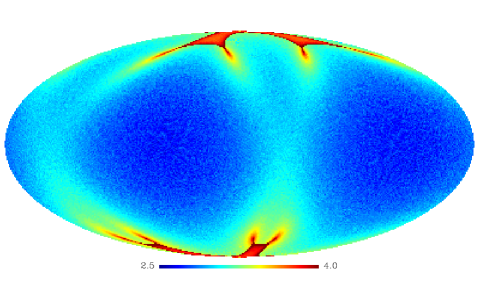
Figure 1: Number of hits per pixel for the scanning strategy applied in this study. The map is in the ecliptic coordinate system. The scale is $\log_{10}(\rm{n_{\rm{hit}}})$, where $\rm{n_{\rm{hit}}}$ is the number of hits in a pixel. (A version of the paper with a better-quality figure can be found at http://www.physics.helsinki.fi/$\sim$tfo$\_$cosm/tfo$\_$planck.html.)

The instrument noise was a sum of white and $1/f$ noise. The PSD of the noise was

$$P(f)=\left(1+\frac{f_{\mathrm{k}}}{f}\right)\frac{\sigma^{2}}{f_{\mathrm{s}}},\quad(f>f_{\mathrm{min}}).$$ (10)

Here $f_{\mathrm{k}}$ is the knee frequency where the spectral powers of the $1/f$ and white noise are equal. The nominal white noise standard deviation (std) per integration time ($t=1/f_{\mathrm{s}}$) is $\sigma$ and $f_{\rm min}$ is the minimum frequency below which the noise spectrum becomes flat. The values of the noise parameters are given in Table 1. They represented a realistic expected noise performance of the instrument hardware. We used the stochastic differential equation (SDE) algorithm (from Level S) to generate the TODs of the instrumental noise. Perfect knowledge of the noise parameter values was assumed both in the ML map-making and in the power spectrum estimation.

Table 1: Simulation parameters used in the TOD generation. Two TODs (signal-only and signal+noise) were generated for all 4 simulation cases leading to 8 TODs in total. The TODs were generated using Level S software (Reinecke et al. Rei05 (2005)). The TODs are sums of CMB (C), foreground (F), and/or noise (N) as indicated in the table. The CMB and foreground TODs were made using totalconvolver and interpolation algorithms (cases 1, 2 and 4) or they were scanned from a high resolution map (case 3). This is also indicated in the table.

Parameters common to all cases
Detector		LFI 100 GHz
Number of detectors		1
Mission time		12 months
Scanning (a)		Cycloidal
Noise
	$\sigma$ (b)	3957.26 $\mu$K
	$f_{\rm min}$	$10^{-4}$ Hz
	$f_{\rm s}$	108.3 Hz

Parameters for	Case 1	Case 2	Case 3	Case 4
TOD (S only)	C+F (c)	C+F (c)	C (d)	C (c)
TOD (S+N)	C+F+N	C+F+N	C+N	C+N
Beam (e,f)	Symmetric	Elliptic	Symmetric	Elliptic
Noise - $f_{\mathrm{k}}$	0.03 Hz	0.03 Hz	0.1 Hz	0.1 Hz

(a) $10\degr$ amplitude and 6 months period.

(b) White noise std of the detector TOD (in antenna temp. units).

(c) Signal made using totalconvolver and interpolation.

(d) Signal scanned from a high resolution map.

(e) Symmetric Gaussian beam:

Full width half maximum (FWHM) = 10.6551 arcmin.

(f) Elliptic Gaussian beam:

FWHMmajor = 11.8652 arcmin, FWHMminor = 9.5684 arcmin.

We used 8 distinct TODs for this study. They were split in four cases (2 TODs in a case). The simulation parameters for the TODs are shown in Table 1. The differences between the cases were the knee frequencies of the instrument noise, the telescope beams, whether the foreground was included, and the ways how the TODs were generated. The sky contained CMB and foreground emissions in cases 1 and 2 but only CMB in cases 3 and 4. Four TODs contained signal+noise and four TODs had signal only. The TODs were convolved with either a symmetric or an elliptic instrument beam (see Table 1).

The CMB signal was derived from a set of $a_{\ell m}$ expansion coefficients that was a realisation from a theoretical CMB angular power spectrum $C_{\ell}^{\rm{th}}$. This $C_{\ell}^{\rm{th}}$ was computed using the CMBFAST code (Seljak & Zaldarriaga Sel96 (1996)), and it corresponds to a $\Lambda$CDM (cosmological constant + Cold Dark Matter) model.

For the cases 1, 2 and 4, the expansion coefficients of the sky were convolved with the beam using the total convolution technique (Wandelt & Górski Wan01 (2001)). The totalconvolver algorithm (part of Level S) outputs a discrete temperature field which is tabulated in an equally spaced three dimensional grid (two dimensions for the pointing of the beam centre and one dimension for the beam orientation). The TOD samples were interpolated from the tabulated temperature grid. For the case 3, the signal TOD was scanned from a high resolution map generated from the $a_{\ell m}$ that had been convolved with the beam. The map had $N_{\rm side}=1024$ and it was generated with the SYNFAST code of the HEALPix package.

4 Output maps

We had 8 TODs available for map-making comprising 4 cases (a signal+noise TOD and a signal-only TOD for each case). Output maps were made from these TODs using three map-making codes, leading to 24 output maps in total.

The 4 cases differed in a number of ways: in whether foreground was included, in noise, in beam shape, and in how TODs were generated. These differences represent both real effects and imperfections (e.g., interpolation errors) in TOD generation. They result in variations of map-making performance from case to case. However, these variations are not the object of this paper. (The TODs differed in too many ways for a study of the effect of these differences to be conducted from just 4 cases). Instead, the object is to compare map-making methods. We have included all 4 cases available to us, mainly to see whether the results of comparison between methods stay consistent from case to case. They do. Some conclusions regarding the effect of foregrounds on the different map-making methods can also be drawn.

All output maps were made with pixel resolution $N_{\rm side}=512$. The noise in the signal+noise TODs resembled the noise of a single LFI 100 GHz detector. Thus the maps are much noisier than they would be if they were made from a full set of 24 detectors, by a factor of about $\sqrt{24}$.

Before the ROMA and MapCUMBA output maps could be made the noise filters had to be produced (see Sect. 2.1). They were determined from the analytical model of the noise PSD (see Eq. (10)) and its known parameter values. The noise filters were symmetric and had $N_{\xi}=65537$ elements at non-negative lags (lag $\geq 0$). The applied noise filters were identical in ROMA and in MapCUMBA. The conjugate gradient iterations were continued until the fractional difference had decreased to $<10^{-6}$.

For destriping the amount of TOD was reduced by averaging 60 scan circles between the repointings. The baseline amplitudes were solved exactly (no iterations) from Eq. (4) using as an additional condition that their sum is zero.

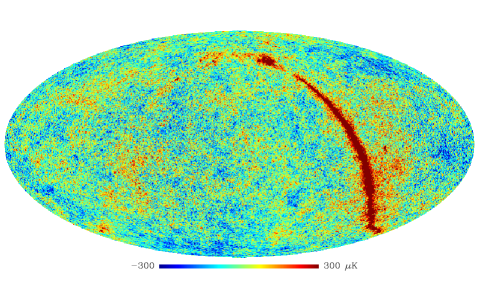
Figure 2: The ROMA output map for case 1. The units are antenna Kelvins at 100 GHz. The maps for MapCUMBA and destriping look similar. This map is an output from one detector. For this plot the map resolution was degraded to $N_{\rm side}=256$. The monopole was removed from the map.

Figure 3: The ROMA reconstruction error map for case 1. The units are antenna Kelvins. The maps for MapCUMBA and destriping look similar. The map is an output from one detector. For this plot the map resolution was degraded to $N_{\rm side}=256$. (A version of the paper with a better-quality figure can be found at http://www.physics.helsinki.fi/$\sim$tfo$\_$cosm/tfo$\_$planck.html.)

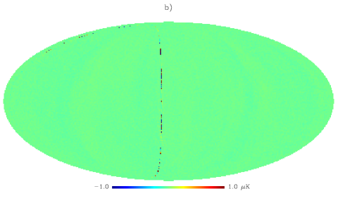
Figure 4: a) Difference map between the output maps of ROMA and destriping. b) Difference map between the output maps of ROMA and MapCUMBA. The pixel minimum, maximum and std values (from the $N_{\rm side}=512$ maps) for map a) are (-109.7, 61.1, 10.0914) $\mu$K and for map b) (-27.4, 38.7, 0.1531) $\mu$K. The units are antenna Kelvins. All maps are for case 1. The corresponding difference map between MapCUMBA and destriping looks similar to map a). For the plots the map resolution was degraded to $N_{\rm side}=256$. (A version of the paper with a better-quality figure can be found at http://www.physics.helsinki.fi/$\sim$tfo$\_$cosm/tfo$\_$planck.html.)

The output maps of ML map-making and destriping can be divided into a binned noiseless map and a reconstruction error map (Tegmark 1997a ). The binned noiseless map is the signal-only TOD binned to map pixels. The reconstruction error map ($\bm{\varepsilon}$) is the (unwanted) deviation of the output map from the binned noiseless map. A goal of map-making is to minimize this error. The reconstruction error map can be further split into the signal ($\bm{\varepsilon}_{p}$) and noise ($\bm{\varepsilon}_{n}$) components: $\bm{\varepsilon}=\bm{\varepsilon}_{p}+\bm{\varepsilon}_{n}$. These are discussed in detail in Appendix A. As shown there, the signal component arises from pixelisation noise (Dóre et al. Dor01 (2001)). The noise component ($\bm{\varepsilon}_{n}$) is the output map from the noise part of the TOD.

Note that the map-making methods are linear (up to numerical accuracy effects), so that these components can be obtained separately and studied independently, by applying the codes to the noise and signal parts of the simulated TODs (see e.g. de Gasperis et al. deG05 (2005)).

Our maps express the temperature fluctuations in the antenna temperature. The ratio of the thermodynamic temperature fluctuation to the antenna temperature fluctuation is $(e^{x}-1)^{2}/x^{2}e^{x}$, where $x=h\nu/kT_{\rm{0}}$, $h$ is the Planck constant, $\nu$ is the frequency, $k$ is the Boltzmann constant and $T_{\rm{0}}$ = 2.725 K is the CMB temperature. For this study the ratio is 1.287 ($\nu$ = 100 GHz).

The output maps and the reconstruction error maps from all three codes look similar. Figs. 2 and 3 show them for case 1. To see the difference, one needs to calculate the difference map between the output maps of the different codes (Fig. 4). The prominent feature in the ROMA - MapCUMBA difference map (see Fig. 4b) falls on top of the last repointing period of the scan. In MapCUMBA the TOD is extended by copying samples from its beginning to the end and vice versa. In ROMA the TOD is extended by padding zeros to the end. The TOD extension is required to make its length suitable for convolution with the noise filter (number of TOD samples to be an integer multiple of $2(N_{\xi}-1)$), but the added samples are not projected on the output map. The feature appearing in the ROMA - MapCUMBA difference map reflects the different treatments of the end of the TOD.

Table 2: The std, minimum and maximum values (all in $\mu$K at 100 GHz antenna scale) of the pixel temperatures of the reconstruction error maps ($\bm{\varepsilon}=\bm{\varepsilon}_{p}+\bm{\varepsilon}_{n}$). The numbers were calculated from $N_{\rm side}=512$ maps. They can be compared to the std of a white noise map, calculated as $\sqrt{\langle 1/n\rangle}\sigma$, where $\langle 1/n\rangle$ is the mean (taken over the hit pixels) of the inverse of the number of hits in a pixel. The values are 137.219 $\mu$K for cases 1 and 2 and 137.400 $\mu$K for cases 3 and 4. The values are different between the cases due to small differences in the cycloidal scannings.This white noise std represents the level below which one cannot get. The difference between ROMA and MapCUMBA is negligible. We give the numbers in the table with many digits just to show at what level this difference is. The numbers in this table and the next one should be compared in the horizontal direction, to see the difference between the codes. The differences in the vertical direction reflect the effect of several differences in how the TODs were generated, but these effects are not the object of this paper.

std for $\bm{\varepsilon}$
(min, max)	ROMA	MapCUMBA	Destriping
Case 1	138.2497	138.2496	138.455
	(-825.3, 876.0)	(-825.3, 876.0)	(-822.5, 891.1)
Case 2	138.2475	138.2474	138.454
	(-825.0, 876.7)	(-825.0, 876.7)	(-822.5, 891.2)
Case 3	138.9109	138.9110	139.397
	(-838.4, 938.2)	(-838.1, 938.1)	(-851.2, 952.3)
Case 4	138.9114	138.9114	139.398
	(-838.1, 937.9)	(-838.1, 937.9)	(-851.2, 952.2)

Table 3: Same as Table 2 but now the values are for the signal component of the reconstruction error map ($\bm{\varepsilon}_{p}$). The units are antenna $\mu$K (at 100 GHz).

std for $\bm{\varepsilon}_{p}$
(min, max)	ROMA	MapCUMBA	Destriping
Case 1	0.8794	0.8796	0.281
	(-100.7, 53.8)	(-100.7, 53.8)	(-3.0, 2.1)
Case 2	0.6140	0.6142	0.252
	(-62.2, 37.8)	(-62.2, 37.8)	(-2.3, 1.8)
Case 3	0.3130	0.3130	0.120
	(-2.0, 1.9)	(-2.0, 1.9)	(-0.6, 0.7)
Case 4	0.4064	0.4064	0.169
	(-2.8, 3.1)	(-2.8, 3.1)	(-0.9, 0.8)

Reconstruction error maps ($\bm{\varepsilon}$) were made by subtracting the binned noiseless map from the signal+noise output maps. Minimum, maximum and std values of the pixel temperatures of the reconstruction error maps are given in Table 2. In terms of the map variance ML map-making is slightly better than destriping. Table 2 also shows that the ML std is higher than the std of the white noise indicating that excess noise remains in the map. The cases 3 and 4 have higher map std’s than the cases 1 and 2. This is mainly caused by the higher knee frequency of the instrument noise in the cases 3 and 4. The map variances of ROMA and MapCUMBA are practically equal showing that their performances are similar. The results shown in Table 2 represent the performance of a single LFI detector. For frequency maps made from the observations of multiple LFI detectors the noise levels would be correspondingly lower. For comparison it can be noted that the noise level of a one-year W-band (94 GHz) frequency map ($N_{\rm side}=512$) of the WMAP experiment (from a total of eight W-band detectors making up 4 differencing assemblies) is slightly higher ($\sim$142 $\mu$K) than the noise levels of Table 2, which represents just a single LFI detector.

Pixel statistics for the signal components of the reconstruction error maps ($\bm{\varepsilon}_{p}$) are given in Table 3. These maps were produced by subtracting the binned noiseless map from the noiseless signal-only output maps. In ML map-making the TOD was convolved with the noise filter. As an example, the signal components of the reconstruction error maps for case 1 are shown in Fig. 5. The maps contained CMB and foreground signals. The error magnitudes are larger for the ML map-making than for the destriping. Additionally, the largest errors in the ML map tend to locate where the foreground signal (actually, its gradient) is strongest. For destriping this error appears as (erroneous) baselines corresponding to offsetting an entire ring. Therefore a similar correlation between the errors and the foreground signal is not visible in the destriped maps, although we expect that the largest errors still originate from where the foreground signal is strong.

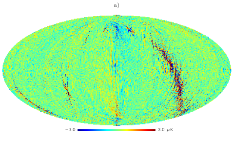
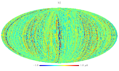
Figure 5: The signal components of the reconstruction error maps for ROMA (a) and for destriping (b). These are difference maps between the signal-only output maps and the binned noiseless maps. The output maps contained CMB and foreground. The units are antenna Kelvins. All maps are for case 1. The corresponding map for MapCUMBA looks similar to map a). The map resolution of the plots is $N_{\rm side}=512$. Note the different colour scales of the maps. (A version of the paper with a better-quality figure can be found at http://www.physics.helsinki.fi/$\sim$tfo$\_$cosm/tfo$\_$planck.html.)

The methods that were used to generate the signal parts of the TODs were not uniform (total convolution vs. scanning of a high resolution map, see Sect. 3). That complicates the comparison of the results of Table 3 between the beams. This comparison was not attempted in this study. However, the results can well be compared (at a given beam) between different map-making algorithms which was the main purpose of this study.

Table 3 shows that the signal-only ML maps deviate more from the binned noiseless map than what happens in destriping. Foreground increases this error and large errors may occur in some pixels of the ML maps. The std of $\bm{\varepsilon}_{p}$ is small compared to the std of the overall reconstruction error map (see Table 2) which is an indication that the total error is dominated by the instrument noise.

The source of $\bm{\varepsilon}_{p}$ is the pixelisation noise (as shown in Appendix A). In ML map-making the pixelisation noise spectrum up to the knee frequency of the instrument noise contributes to $\bm{\varepsilon}_{p}$. In destriping, however, only a lower frequency part contributes leading to a smaller $\bm{\varepsilon}_{p}$. This is addressed in more detail in Appendix A. The galactic foreground signal has a stronger spatial variation than CMB. This results in higher pixelisation noise, which explains the higher $\bm{\varepsilon}_{p}$ magnitudes in the cases 1 and 2 than in the cases 3 and 4 (see Table 3).

We calculated the angular power spectra of the reconstruction error maps ($\bm{\varepsilon}$) (Fig. 6). The spectra of ROMA and MapCUMBA were very similar and could not be distinguished in the plot. The ratio of the power spectra between destriping and ROMA is shown in Fig. 7. It seems that in destriping $\bm{\varepsilon}$ has higher power in most multipoles.

To examine this further, 100 MC noise-only TODs were produced from the known PSD of the instrument noise (see Eq. (10)). The MC noise TODs were generated by the SDE method using a different seed value for every realisation. To have a reasonable calculation time for this MC study, multiple 35 hour chunks of noise were generated simultaneously in parallel processing and the chunks were glued one after another at the end. This leads to an MC noise TOD with no correlation between the chunks. Because the correlation of the noise in the observed TODs is weak at $>$ 35 hour lags, the zero correlation beyond 35 hours in the MC noise is expected to cause an insignificant error in the noise bias estimates.

Output maps for ROMA and destriping were made from the MC noise TODs and their angular spectra were derived. The mean spectra are shown in Fig. 8. It shows that the mean angular power is higher in destriping at all scales. The lower power at some $\ell$ (in Fig. 7) seems to be just due to random variation.

The map-making codes were run on an IBM SP RS/6000 computer with a cluster of Power3 processors running at a clock speed of 375 MHz. ROMA and MapCUMBA codes were run parallel in multiple processors (number of processors was typically between 192 and 256) and it took $\sim$10 min to produce an ML output map. In destriping an output map was produced in $\sim$7 min in a single processor job. In MC studies this time can be reduced to $\sim$4 min by inverting the matrix (see Eq. (4)) once and using the inverse in the subsequent runs.

Note that a part of this large difference in computation cost is due to destriping being applied to a coadded TOD, which was a factor 60 shorter than a full TOD. This coadding was possible without error, because we assumed idealized pointing. In reality, the pointings of the different circles of the same ring do not fall exactly on top of each other. This means that either some additional error is introduced by the coadding, or that destriping has to work with the actual pointings of the full TOD. The latter option increases the computational cost of destriping, but it will still be significantly less than for ML map-making.

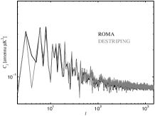
Figure 6: The angular power spectra of the reconstruction error maps ($\bm{\varepsilon}$) for ROMA and destriping. The angular power spectra for ROMA and MapCUMBA were very similar and would be on top of each other in this plot. The curves are for case 4.

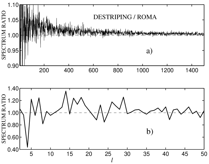
Figure 7: The ratio of the angular power spectra of Fig. 6. a) Full curve. b) Zoom to low $\ell$.

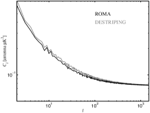
Figure 8: Mean angular power spectra of output maps from 100 MC realisations of noise TODs. The realisations were derived from the known PSD of the instrument noise (see Eq. (10)). Because the MC TODs were noise-only, this plot is for cases 3 and 4.

5 Power spectrum estimates

To see how the differences between destriping and ML map-making are reflected in the angular power spectrum estimates, we derived $C_{\ell}$ estimates from the output maps of case 3, where the TOD contained CMB and noise. Since the output maps from ROMA and MapCUMBA were practically identical, we let ROMA represent ML map-making in this section. The CMB was convolved with the symmetric beam (case 3, see Table 1). As defined in Sect. 2.3, our power spectrum estimates $\widehat{C}_{\ell}^{\rm B}$ are estimates of the angular power spectrum of the binned noiseless map. The estimates were compared to the actual spectrum ($C_{\ell}^{\rm B}$) of the binned noiseless map. That map was binned from the noiseless TOD containing CMB only. The angular spectrum $C_{\ell}^{\rm B}$ is shown in Fig. 9, which also shows the input spectrum $C_{\ell}^{\rm in}$. The difference between $C_{\ell}^{\rm B}$ and $C_{\ell}^{\rm in}$ is due to a number of effects, which are discussed in Appendix B; but they are not relevant for our comparison between map-making methods, as they can only produce estimates of $C_{\ell}^{\rm B}$.

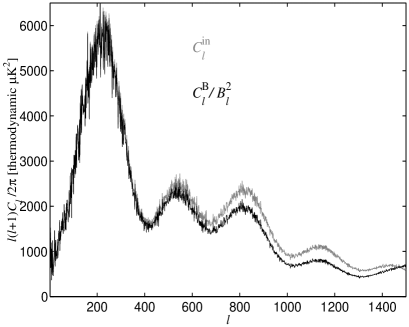
Figure 9: The angular power spectrum ($C_{\ell}^{\rm B}$) of the binned noiseless map (black curve). The map ($N_{\rm side}=512$) was binned from the simulated noiseless TOD containing CMB that was smoothed with the symmetric beam (case 3, see Table 1). The $C_{\ell}^{\rm B}$ spectrum shown in the plot is deconvolved with the same symmetric beam response. For comparison, the input power spectrum $C_{\ell}^{\rm{in}}$ of the CMB sky is shown as well (grey curve). The difference between $C_{\ell}^{\rm B}$ and $C_{\ell}^{\rm{in}}$ is (in this case) mainly due to pixel window smoothing and is discussed in Appendix B.

The relation between the pseudo spectrum $\widetilde{C}_{\ell}$ (angular power spectrum obtained from the output map) and the power spectrum estimate ($\widehat{C}_{\ell}^{\rm B}$) was given in Eq. (9). The estimate is obtained by inverting the equation. The estimate of the noise bias $\langle\widetilde{N}_{\ell}\rangle$ was obtained from the MC simulations (see Fig. 8). The value of $F_{\ell}$ was initially set to one. The obtained power spectrum estimates, the spectrum of the binned noiseless map and the MC noise bias (for destriping) are shown in Fig. 10.

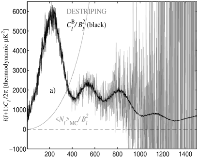
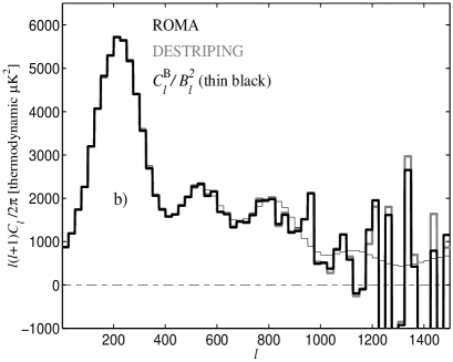
Figure 10: a) Angular power spectrum estimate $\widehat{C}_{\ell}^{\rm B}$ for destriping (grey curve). The ROMA estimate would fall nearly on top of the destriping estimate and would not distinguish in this plot. The estimates were derived from a single sky realisation (case 3). The output maps covered the full sky and contained CMB and instrument noise. Since just a single detector was considered, the noise becomes dominant already at around $\ell\simeq 350$. $C_{\ell}^{\rm{B}}$ is the angular spectrum of the binned noiseless map and $\langle N_{\ell}\rangle_{\rm{MC}}$ is the MC noise bias (for destriping). Note that they have been deconvolved with a symmetric beam that was identical to the instrument beam. The filter function $F_{\ell}$ was set to one for both estimates. b) Same as a) but the spectra have been $\ell$ binned to $\Delta\ell=25$. The difference between the ROMA and destriping estimates is visible at $\ell>1000$.

For the quality of an angular power spectrum estimate its bias and covariance matrix are important figures of merit. For the covariance matrix we restricted our study to its diagonal elements, which represent the error bars of the estimate.

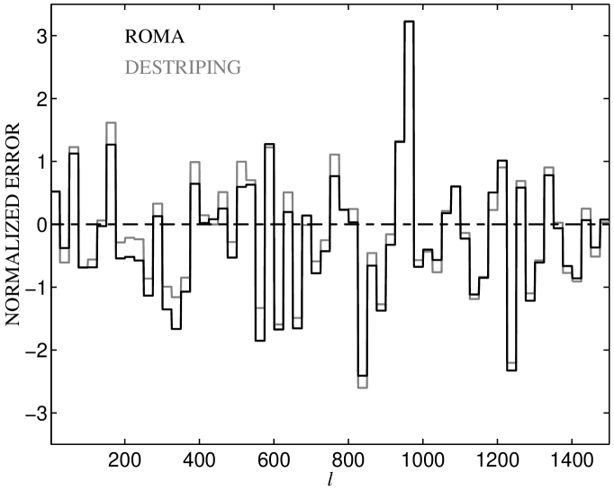
Figure 11: The normalized power spectrum estimation errors for ROMA and destriping. The normalized error was obtained by dividing the binned estimation error (Eq. (11), $\Delta\ell=25$) with the analytic approximation of its std (Eq. (12)). The std of destriping was used in all normalizations. The filter function had value 1.0 for both curves. The bin-to-bin fluctuations are mainly caused by the instrument noise.

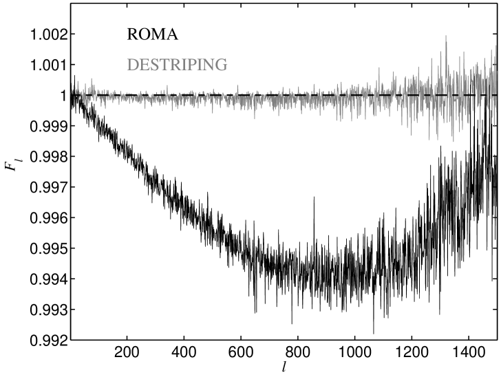
Figure 12: Filter functions $F_{\ell}$ for ROMA and destriping. They were obtained from Eq. (9) (with $\langle\widetilde{N}_{\ell}\rangle=0$) by dividing the pseudo spectra of the output maps of the noiseless CMB-only TOD with the spectrum of the binned noiseless map. The filter function for MapCUMBA was nearly identical to the filter function of ROMA and would not distinguish from the ROMA filter function in this plot.

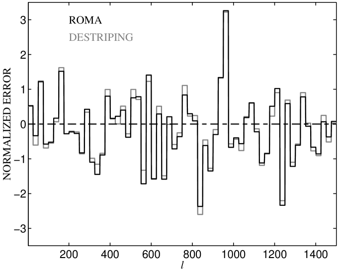
Figure 13: Same as Fig. 11 but now the power spectrum estimates have been corrected with the estimates of the filter function (from Fig. 12).

5.1 Bias

We defined the estimation error $\Delta\widehat{C}_{\ell}$ as the difference between the power spectrum estimate and the spectrum of the binned noiseless map: $\Delta\widehat{C}_{\ell}=\widehat{C}_{\ell}^{\rm B}-C_{\ell}^{\rm{B}}$. The estimation error was binned by averaging $\Delta\ell$ multipoles to a bin

$$\Delta\widehat{\mathcal{C}}_{b}=\frac{1}{\Delta\ell}\sum_{\ell\in b}{\frac{\ell(\ell+1)\Delta\widehat{C}_{\ell}}{2\pi}}.$$ (11)

We evaluated the binned errors $\Delta\widehat{\mathcal{C}}_{b}$ for ROMA and destriping from the spectra shown in Fig. 10. To facilitate the comparison of the binned estimation errors, we normalized them by dividing them with an analytic approximation of their std, which was obtained from

$$\sigma_{b}=\left[\frac{1}{{\Delta\ell}^{2}}\sum_{\ell\in b}{\left(\frac{\ell(\ell+1)}{2\pi}\right)^{2}\sigma_{\ell}^{2}}\right]^{1/2},$$ (12)

where

$$\sigma_{\ell}=\sqrt{\frac{2}{(2\ell+1)f_{\rm{sky}}}\left(2C_{\ell}^{\rm{B}}\langle\widetilde{N}_{\ell}\rangle+\langle\widetilde{N}_{\ell}\rangle^{2}\right)}.$$ (13)

is the approximation for the std of the unbinned error $\Delta\widehat{C}_{\ell}$ (Efstathiou Efs05 (2005)). In this formula $C_{\ell}^{\rm B}$ is a given signal (no cosmic variance). Sky coverage fraction is $f_{\rm{sky}}=1$ in our case. For all normalizations we used the $\langle\widetilde{N}_{\ell}\rangle_{\rm{MC}}$ obtained for destriping in place of $\langle\widetilde{N}_{\ell}\rangle$.

The normalized errors are shown in Fig. 11. Their std (from one noise realisation to another) should be $\sim$1. If an angular power spectrum estimate has a non-zero bias the mean of the fluctuations of the normalized error will have a positive or negative trend. In the case of zero bias the mean will be close to zero. We can note that the normalized errors are different for ROMA and destriping, the largest differences being at $\ell<800$. The differences are, however, smaller than the std of the errors.

We could expect that some bias could be introduced to our power spectrum estimates because we neglected (by setting $F_{\ell}$ = 1 in Eq. (9)) the error that the map-making causes to the CMB signal. This is a reflection of the signal component $\bm{\varepsilon}_{p}$ of the reconstruction error that we found in the map domain (see Sect. 4). To assess the level of the bias we estimated $F_{\ell}$ for ROMA and for destriping. We carried out no MC simulations to estimate them, but we determined them from Eq. (9) using the pseudo spectra $\widetilde{C}_{\ell}$ from the output maps of the noiseless (CMB-only) TOD ($\langle\widetilde{N}_{\ell}\rangle=0$). Because the values of $F_{\ell}$ are based on one CMB realisation only, these results should be taken as indicative. (In fact, we now fully correct for the effect of $\bm{\varepsilon}_{p}$, since the filter function is derived from the same realisation to which it is applied. In reality, of course, the signal-only TOD will not be available, and the filter function should be evaluated as an expectation value. It will then remove only the bias due to $\bm{\varepsilon}_{p}$.)

The obtained $F_{\ell}$ are shown in Fig. 12. For destriping there is essentially no filter function ($F_{\ell}\sim 1$, Poutanen et al. Pou04 (2004)). For ROMA the deviation from 1 is larger, showing its largest values at $\ell=800\ldots 1000$. If not corrected, the map-making errors cause a bias in the ML spectrum estimates whose maximum value in this case would be $\sim$0.6% of the magnitude of the CMB spectrum.

We corrected our angular power spectrum estimates with the obtained $F_{\ell}$ and reproduced the normalized estimation errors. The result is shown in Fig. 13. When comparing to Fig. 11 the improved match between the normalized errors of ROMA and destriping can be noted (especially at $\ell<600$). The remaining differences are mainly due to the differences in the noise of the output maps of these two algorithms.

5.2 Error bars

An error bar is defined here as the square root of the diagonal element of the covariance matrix $\langle\Delta\widehat{C}_{\ell}\Delta\widehat{C}_{\ell^{\prime}}\rangle$ ($\pm 1\sigma$ error bar). The error bars can be derived either analytically (Tegmark 1997b ; Efstathiou Efs04 (2004)) or by MC simulations (Hivon et al. Hiv02 (2002); Poutanen et al. Pou04 (2004)). In this study we did not do signal+noise MC simulations to determine the error bars, but used instead an approximation to compare ROMA and destriping. We used $\sigma_{\ell}$ from Eq. (13) with a modification that takes into account the different filter functions for different map-making algorithms ($F_{\ell}$ assumed value 1.0 in Eq. (13))

$$\sqrt{\langle(\Delta\widehat{C}_{\ell})^{2}\rangle}=\sqrt{\frac{2}{(2\ell+1)}}\sqrt{\frac{2F_{\ell}C_{\ell}^{\rm{B}}\langle\widetilde{N}_{\ell}\rangle_{\rm{MC}}+\langle\widetilde{N}_{\ell}\rangle_{\rm{MC}}^{2}}{F_{\ell}^{2}}}.$$ (14)

The spectrum $C_{\ell}^{\rm B}$ represents here a given signal (no cosmic variance).

Applying the spectrum $C_{\ell}^{\rm B}$ from Fig. 9, the noise biases ($\langle\widetilde{N}_{\ell}\rangle_{\rm{MC}}$) from Fig. 8 and the filter functions from Fig. 12 the ratio of the error bars between destriping and ROMA was evaluated. It is shown in Fig. 14 (black curve). The error bars at $\ell\lesssim 1000$ are larger for destriping than for ROMA. The largest relative differences are $\sim$5%. The main cause of the larger error bars is the higher level of noise in the output maps of destriping (see Table 2). At high-$\ell$ the larger map noise of the destriping is partly compensated by its larger filter function (see Fig. 12) leading to error bars that have nearly the same magnitude as the ROMA error bars.

As a second case we assumed that we want to estimate the angular spectrum $C_{\ell}^{\mathrm{th}}$ of the underlying theoretical CMB (instead of its particular realisation as above). Cosmic variance then increases the error bars (Scott et al. Sco94 (1994); Hobson & Magueijo Hob96 (1996)):

$$\sqrt{\langle(\Delta\widehat{C}_{\ell})^{2}\rangle}=\sqrt{\frac{2}{(2\ell+1)}}\frac{F_{\ell}C_{\ell}^{\rm{B}}+\langle\widetilde{N}_{\ell}\rangle_{\rm{MC}}}{F_{\ell}}.$$ (15)

The ratio of these error bars is shown in Fig. 14 as well (grey curve). Because noise dominates the error bars at high multipoles, these are similar to the error bars without cosmic variance. Due to the dominance of cosmic variance at low multipoles, the magnitudes of the error bars of the two methods approach each other at low $\ell$.

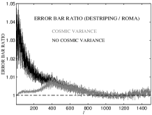
Figure 14: An estimate for the ratio of the error bars between destriping and ROMA. Black curve is for the estimation of a particular CMB realisation of the sky (no cosmic variance, error bars from Eq. (14)) and the grey curve is for the estimation of the underlying theoretical CMB spectrum (cosmic variance included, error bars from Eq. (15)).

6 Conclusions

We have presented a comparison of the maps produced by three different map-making codes and two map-making methods, destriping and ML map-making. We also compared the angular power spectrum estimates obtained from destriping and ML maps. The maps and power spectra were derived from a set of one-year TOD streams that resembled the observations expected from a single 100 GHz Planck LFI detector.

In terms of the map variance the two ML codes, ROMA and MapCUMBA, produce nearly identical maps, with lower noise than destriping. This lower noise is an advantage for them and it facilitates smaller error bars for the power spectrum estimates. The difference is, however, rather small.

ROMA and MapCUMBA require knowledge of the power spectrum of the instrument noise, whereas destriping does not. In a real experiment the noise spectrum (if required) needs to be estimated from the observed data. Some estimation error can be expected which may increase the noise in the ROMA and MapCUMBA maps. Thus differences in the noise performance between ROMA/MapCUMBA and destriping may become smaller in a real experiment. A perfectly known instrument noise spectrum was assumed in this study.

The map-making methods caused errors (exhibited in the signal component of the reconstruction error map) in the signal part of the output maps. The origin of these errors is the sub-pixel structure of the signal (pixelisation noise). It was shown that these errors were smaller in destriping than in ROMA and MapCUMBA. It was further shown that, if a proper correction is not applied, these errors may show up as an extra bias in the power spectrum estimates. The extra bias would be larger for ROMA and MapCUMBA than for destriping.

In terms of CPU resources destriping is less demanding. This is an advantage in e.g. MC simulations.

Appendix A Reconstruction error map

In this Appendix we discuss in more detail the reconstruction error map and how its signal and noise components arise.

The output map of the ML map-making can be solved from Eq. (2). That equation is reproduced here

$$\mathbf{P}^{T}\mathbf{N}^{-1}\mathbf{P}{\mathbf{m}}=\mathbf{P}^{T}\mathbf{N}^{-1}{\mathbf{y}}.$$ (16)

The noise covariance matrix $\mathbf{N}$ can be freely normalized by a constant without affecting the output map. Let us assume that each element of $\mathbf{N}$ has been divided by the variance ($\sigma^{2}$) of the non-correlated noise component of the observed TOD (vector ${\mathbf{y}}$). By replacing $\mathbf{N}^{-1}$ with an identity $\mathbf{I}_{t}-(\mathbf{I}_{t}-\mathbf{N}^{-1})$ and rearranging some of the terms one obtains for the output map

$${\mathbf{m}}=(\mathbf{P}^{T}\mathbf{P})^{-1}\mathbf{B}^{-1}\mathbf{P}^{T}\mathbf{N}^{-1}{\mathbf{y}},$$ (17)

where

$$\mathbf{B}=\mathbf{I}_{m}-\mathbf{P}^{T}(\mathbf{I}_{t}-\mathbf{N}^{-1})\mathbf{P}(\mathbf{P}^{T}\mathbf{P})^{-1}.$$ (18)

Here $\mathbf{I}_{t}$ and $\mathbf{I}_{m}$ are unit matrices with dimensions equal to the number of samples $N_{t}$ of the TOD and the number of pixels $N_{\rm{pix}}$ in the map, respectively. We can apply a geometric series trick (Tegmark 1997a ) to prove the following identity

$$[\mathbf{I}_{m}-\mathbf{P}^{T}(\mathbf{I}_{t}-\mathbf{N}^{-1})\mathbf{P}(\mathbf{P}^{T}\mathbf{P})^{-1}]^{-1}\mathbf{P}^{T}=$$

$$=\mathbf{P}^{T}[\mathbf{I}_{t}-(\mathbf{I}_{t}-\mathbf{N}^{-1})\mathbf{P}(\mathbf{P}^{T}\mathbf{P})^{-1}\mathbf{P}^{T}]^{-1}.$$ (19)

Applying this in Eqs. (17) and (18) and noting the definition of the matrix $\mathbf{Z}$ (see Sect. 2.2) one obtains for the output map

$${\mathbf{m}}=(\mathbf{P}^{T}\mathbf{P})^{-1}\mathbf{P}^{T}[\mathbf{I}_{t}+(\mathbf{N}-\mathbf{I}_{t})\mathbf{Z}]^{-1}{\mathbf{y}}.$$ (20)

By adding and subtracting ${\mathbf{y}}$ on the right hand side and carrying out some arithmetic manipulations the output map can be expressed in the following form

$${\mathbf{m}}=(\mathbf{P}^{T}\mathbf{P})^{-1}\mathbf{P}^{T}[{\mathbf{y}}-{\mathbf{\Delta}}].$$ (21)

Vector ${\mathbf{\Delta}}$ is solved from the linear equation

$$[\mathbf{Z}+(\mathbf{N}-\mathbf{I}_{t})^{-1}]{\mathbf{\Delta}}=\mathbf{Z}{\mathbf{y}}.$$ (22)

Let the complex valued matrix $\mathbf{H}$ ($[H]=(N_{t},N_{t})$) be an inverse DFT (Discrete Fourier Transform) operator that converts frequency domain vectors to time domain (to TOD domain): ${\mathbf{y}}=\mathbf{H}\widetilde{{\mathbf{y}}}$, where $\widetilde{{\mathbf{y}}}$ is the frequency domain counterpart of ${\mathbf{y}}$. The inverse operator to $\mathbf{H}$ is its Hermitian conjugate $\mathbf{H}^{{\dagger}}$. We can assume that the matrix $\mathbf{H}$ is normalized to $\mathbf{H}\mathbf{H}^{{\dagger}}=\mathbf{H}^{{\dagger}}\mathbf{H}=\mathbf{I}_{t}$. A square matrix $\mathbf{A}$ ($[A]=(N_{t},N_{t})$) in the TOD domain can be converted to a matrix $\widetilde{\mathbf{A}}$ in the frequency domain: $\widetilde{\mathbf{A}}=\mathbf{H}^{{\dagger}}\mathbf{A}\mathbf{H}$.

After converting both sides of Eq. (22) into frequency domain, the vector $\widetilde{{\mathbf{\Delta}}}$ (frequency domain counterpart of ${\mathbf{\Delta}}$) can be solved from the equation

$$[\mathbf{H}^{{\dagger}}\mathbf{Z}\mathbf{H}+(\widetilde{\mathbf{N}}-\mathbf{I}_{t})^{-1}]\widetilde{{\mathbf{\Delta}}}=\mathbf{H}^{{\dagger}}\mathbf{Z}{\mathbf{y}}.$$ (23)

The solution for the output map becomes then

$${\mathbf{m}}=(\mathbf{P}^{T}\mathbf{P})^{-1}\mathbf{P}^{T}[{\mathbf{y}}-\mathbf{H}\widetilde{{\mathbf{\Delta}}}].$$ (24)

Comparing Eqs. (23) and (24) to the corresponding Eqs. (4) and (5) of destriping the similarity of the output map solutions between ML and destriping can be clearly seen.

The observed TOD (${\mathbf{y}}$) contains two components: signal ${\mathbf{s}}$ and instrument noise ${\mathbf{n}}$ (see Sect. 3). The term $\mathbf{Z}{\mathbf{y}}$ (see Eq.  (23)) can now be split in two components

$$\mathbf{Z}{\mathbf{y}}=\mathbf{Z}{\mathbf{s}}+\mathbf{Z}{\mathbf{n}}.$$ (25)

Writing out the first term on the right hand side we obtain

$$\mathbf{Z}{\mathbf{s}}={\mathbf{s}}-\mathbf{P}(\mathbf{P}^{T}\mathbf{P})^{-1}\mathbf{P}^{T}{\mathbf{s}}.$$ (26)

Apart from the sign, $\mathbf{Z}{\mathbf{s}}$ is the pixelisation noise introduced by Doré et al. (Dor01 (2001)). Pixelisation noise represents error that is caused by the discretization of the sky into pixels. Following Doré et al. (Dor01 (2001)) we define pixelisation noise ${\mathbf{p}}=-\mathbf{Z}{\mathbf{s}}$.

The split of $\mathbf{Z}{\mathbf{y}}$ in two components means that $\widetilde{{\mathbf{\Delta}}}$ is split in two components as well: $\widetilde{{\mathbf{\Delta}}}=\widetilde{{\mathbf{\Delta}}}_{p}+\widetilde{{\mathbf{\Delta}}}_{n}$. They can be solved from

$$[\mathbf{H}^{{\dagger}}\mathbf{Z}\mathbf{H}+(\widetilde{\mathbf{N}}-\mathbf{I}_{t})^{-1}]\widetilde{{\mathbf{\Delta}}}_{p}=-\mathbf{H}^{{\dagger}}{\mathbf{p}}$$ (27)

and

$$[\mathbf{H}^{{\dagger}}\mathbf{Z}\mathbf{H}+(\widetilde{\mathbf{N}}-\mathbf{I}_{t})^{-1}]\widetilde{{\mathbf{\Delta}}}_{n}=\mathbf{H}^{{\dagger}}\mathbf{Z}{\mathbf{n}}.$$ (28)

In destriping the amplitudes of the base functions are split analogously: ${\mathbf{a}}={\mathbf{a}}_{p}+{\mathbf{a}}_{n}$. The first component is determined by the pixelisation noise and the second one by the instrument noise.

Next we insert ${\mathbf{y}}={\mathbf{s}}+{\mathbf{n}}$ into Eqs. (21) and (22). We obtain for the output map

$${\mathbf{m}}=(\mathbf{P}^{T}\mathbf{P})^{-1}\mathbf{P}^{T}{\mathbf{s}}-(\mathbf{P}^{T}\mathbf{P})^{-1}\mathbf{P}^{T}\mathbf{H}\widetilde{{\mathbf{\Delta}}}_{p}+$$

$$+(\mathbf{P}^{T}\mathbf{P})^{-1}\mathbf{P}^{T}[{\mathbf{n}}-\mathbf{H}\widetilde{{\mathbf{\Delta}}}_{n}].$$ (29)

Ideally, we would like the output map of the map-making algorithm to be equal to the first term on the right hand side. It is called binned noiseless map in this study. The rest of the terms bring error. They are represented by the reconstruction error map (Tegmark 1997a )

$$\bm{\varepsilon}={\mathbf{m}}-(\mathbf{P}^{T}\mathbf{P})^{-1}\mathbf{P}^{T}{\mathbf{s}}.$$ (30)

The reconstruction error map is comprised of a signal component ($\bm{\varepsilon}_{p}$) and a noise component ($\bm{\varepsilon}_{n}$).

$$\bm{\varepsilon}=\bm{\varepsilon}_{p}+\bm{\varepsilon}_{n}.$$ (31)

$$\bm{\varepsilon}_{p}=-(\mathbf{P}^{T}\mathbf{P})^{-1}\mathbf{P}^{T}\mathbf{H}\widetilde{{\mathbf{\Delta}}}_{p}$$ (32)

$$\bm{\varepsilon}_{n}=(\mathbf{P}^{T}\mathbf{P})^{-1}\mathbf{P}^{T}[{\mathbf{n}}-\mathbf{H}\widetilde{{\mathbf{\Delta}}}_{n}]$$ (33)

For destriping we can write analogously

$$\bm{\varepsilon}_{p}=-(\mathbf{P}^{T}\mathbf{P})^{-1}\mathbf{P}^{T}\mathbf{F}{\mathbf{a}}_{p}$$ (34)

$$\bm{\varepsilon}_{n}=(\mathbf{P}^{T}\mathbf{P})^{-1}\mathbf{P}^{T}[{\mathbf{n}}-\mathbf{F}{\mathbf{a}}_{n}].$$ (35)

The signal and noise components of the reconstruction error map were used extensively when the map-making algorithms were compared in Sect. 4. We studied the minimum, maximum and std values of their pixel temperatures. Additionally, we produced their angular power spectra and compared them as well.

A.1 Map-making errors and pixelisation noise

The purpose of this section is to give a qualitative explanation to the fact that the magnitude of the signal component of the reconstruction error map is larger for the ML map-making than for the destriping. The signal component of the reconstruction error depends on $\widetilde{{\mathbf{\Delta}}}_{p}$ in the ML map-making and on ${\mathbf{a}}_{p}$ in the destriping (see Eqs. (32) and (34)). The source of both quantities is the pixelisation noise ${\mathbf{p}}$.

We will first examine the spectrum of the pixelisation noise ($\tilde{{\mathbf{p}}}=\mathbf{H}^{{\dagger}}{\mathbf{p}}$). The PSD of every 60 circle averaged ring of a simulated signal-only TOD was calculated and the mean of these PSDs was taken over the full one year TOD. The mean PSDs of all four simulated signal-only TODs and their associated pixelisation noise streams (${\mathbf{p}}=-\mathbf{Z}{\mathbf{s}}$, ${\mathbf{s}}$ = TOD) were determined. They are shown in Fig. 15.

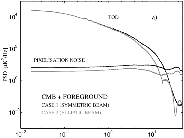
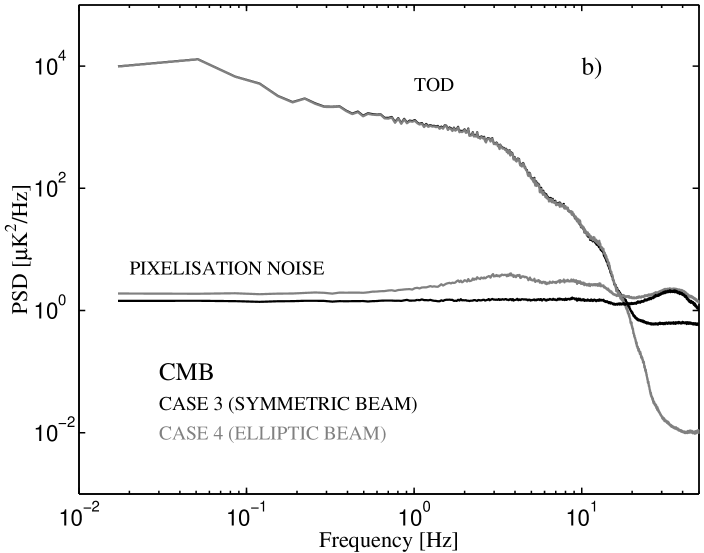
Figure 15: The PSD of every 60 circle averaged ring of a simulated signal-only TOD was calculated (8766 PSDs for a TOD) and the mean of the PSDs was taken. The mean PSDs of all signal-only TODs generated for this study are shown (curves labeled with ”TOD”). The mean PSDs of the associated pixelisation noise streams were calculated as well and are shown too. a) TOD contains CMB and foreground. b) TOD contains only CMB. The temperature units are antenna $\mu$K at 100 GHz.

The level of the pixelisation noise is higher for the TODs containing CMB and foreground than for the TODs of CMB only. This explains why the signal component of the reconstruction error increases when the foreground emissions are included in the simulations.

The sample $p_{k}$ of the pixelisation noise stream ($k$ indexes the sample) is

$$p_{k}=\left(\frac{1}{N_{k}}\sum_{i\in k}s_{i}\right)-s_{k}=\frac{1}{N_{k}}\sum_{i\in k}(s_{i}-s_{k}),$$ (36)

where $s_{k}$ is the k^th sample of the TOD, $i\in k$ refers to those TOD samples (including $s_{k}$) that hit the same pixel as $s_{k}$ and $N_{k}$ is the number of hits in that pixel. We can assume that the magnitudes of the pixel-to-pixel correlations are smaller for the temperature differences ($s_{i}-s_{k}$) than for the temperatures themselves. This means that notable correlation exists between $p_{k}$ and $p_{k^{\prime}}$ only if they are samples from the same pixel. Only the fraction $N_{\rm pix}/N_{\rm t}\ll 1$ of the TOD samples are observations from the same pixel leading to, in average, a weak correlation between the samples of the pixelisation noise. This explains the ”white noise” type nearly flat spectra of the pixelisation noises (see Fig. 15). The fact that in Fig. 15a the pixelisation noise is larger for the symmetric beam than for the elliptic beam and opposite in Fig. 15b reflects the different methods that were used in generating the symmetric beam TODs (total convolution in case 1 vs. scanning a high resolution map in case 3, see Sect. 3).

Vector $\widetilde{{\mathbf{\Delta}}}_{p}$ is a solution to Eq. (27). The matrix $\widetilde{\mathbf{N}}$ is diagonal with samples (bins) of $1+f_{\mathrm{k}}/f$ (cf. Eq. (10)) in its diagonals. The diagonal elements of $(\widetilde{\mathbf{N}}-\mathbf{I}_{t})^{-1}$ are $\gg 1$ for frequencies higher than the knee frequency. Fig. 15 suggests that the power of $\mathbf{H}^{{\dagger}}\mathbf{Z}\mathbf{H}\widetilde{{\mathbf{\Delta}}}_{p}$ is considerably smaller than the power of $\widetilde{{\mathbf{\Delta}}}_{p}$ leading to an approximation where we can ignore $\mathbf{H}^{{\dagger}}\mathbf{Z}\mathbf{H}$ in Eq. (27). This indicates that in the ML map-making the signal component of the reconstruction error is mainly determined by that part of the pixelisation noise spectrum that falls below the knee frequency (Hivon et al. Hiv05 (2005)).

By looking at Eqs. (4) and (34) we can expect that in destriping the uniform baselines of the pixelisation noise contribute to this error. Because we assumed an exact repetition of the pointings of the 60 circles of a ring, the pixelisation noise of those circles is periodic (with period $T$ = 60 s) and it has a Fourier series representation whose Fourier mode frequencies are multiples of $1/T$. The lowest (zero) mode contributes to the uniform baselines, whereas the modes up to the knee frequency (0.1 Hz) contribute to the reconstruction error of the ML map-making. This explains why the signal component of the reconstruction error is smaller in destriping than in ML map-making. The evaluation of the exact effect in the maps is complicated by the scanning strategy.

Appendix B Pixel window and pointing distribution effects

There are a number of effects contributing to the difference between the input spectrum $C_{\ell}^{\rm{in}}$ and that of the binned noiseless map $C_{\ell}^{\rm{B}}$. For cases 1, 2 and 4 these include the beam shape, spectrum smoothing due to sample interpolation from the totalconvolver temperature grid (see Sect. 3) and the effective elongation of the beam due to sample integration. The sample integration was simulated in Level S by generating multiple (fast) samples at a higher sampling rate and the final output sample of the detector (at sampling rate $f_{\rm s}$) was an average (with equal weights) of the fast samples.

In case 3 the interpolation and sample integration errors do not occur, because the signal part of the TOD was made by picking the temperatures (at sampling rate $f_{\rm s}$) from a high-resolution input map, which was smoothed by a spherical beam. Thus the only beam effect was that of the spherical beam, which we already corrected for in Fig. 9. The input spectrum displayed in Fig. 9 is actually that of this input map, corrected for the beam.

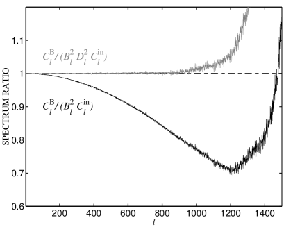
Figure 16: The ratio of the spectra shown in Fig. 9 (black curve). The grey curve shows the same ratio after the spectrum of the binned map ($C_{\ell}^{\rm B}$) has been deconvolved with an approximate pixel window of the binning: $D_{\ell}^{2}=D_{\ell}^{2}(512)/D_{\ell}^{2}(1024)$.

Another effect comes from how the detector pointings sample the sky, or, in this case (case 3), the small pixels of the input map, to produce the binned map with its larger pixel size (the same as the output map). In case 3 the input map had $N_{\mathrm{side}}=1024$, whereas the binned map had $N_{\mathrm{side}}=512$, so that each pixel of the binned map can be divided into four subpixels corresponding to the pixels of the input map. (Note that the discussion in Sect. 2 on map-making methods assumed the same pixel size for input and output maps, and therefore did not recognize the effects discussed here.) If each of the 4 subpixels had been hit by the same number of times, the resulting binned noiseless map would be just the input map downgraded to $N_{\mathrm{side}}=512$. The effect on the map spectrum should then be given by the ratio of the two pixel windows $D_{\ell}^{2}(512)/D_{\ell}^{2}(1024)$. Here $D_{\ell}(512)$ and $D_{\ell}(1024)$ are the HEALPix pixel window functions for $N_{\rm side}$ = 512 and $N_{\rm side}$ = 1024 (Górski et al. 2005b ). (In the real situation the input map is replaced by the sky with “$N_{\mathrm{side}}=\infty$”, so that the corresponding factor is just the pixel window of the binned map.) We show in Fig. 16 how this represents the effect well up to $\ell\sim 800$.

The remaining effect, which blows up at high $\ell$, is due to two things: 1) the nonuniform sampling of the four subpixels (or, in the real world, that of the output map pixel area on the sky), 2) that the HEALPix pixel window functions themselves represent an approximation, as discussed below. This remaining effect represents coupling between the $\ell$ modes of the spectra, which couples power from the low-$\ell$ to the high-$\ell$ that shows up as an high-$\ell$ excess power. This effect was discussed in Poutanen et al. Pou04 (2004), where it was modelled as a signal bias.

Let us examine the distribution of the detector pointings in the sky and its impact on the spectrum of the binned noiseless map in more detail. The following discussion can be applied both to the real case of observing the sky and the case (our case 3) where the TOD is picked from a high-resolution pixelized input map. We consider the samples $s_{i}$ ($i$ indexes the sample) of the CMB-only TOD that fall in a pixel $k$ of the binned (or output) map (see Eq. (36)). The number of hits in that pixel is $N_{k}$. We assume that every pixel is hit (100% sky coverage at $N_{\rm side}=512$ resolution), so that $N_{k}\geq 1$. The temperature of $s_{i}$ can be given as

$$s_{i}=\sum_{\ell m}{a_{\ell m}B_{\ell}Y_{\ell m}({\mathbf{n}}_{i})}.$$ (37)

Here $a_{\ell m}$ represent the CMB sky (see Sect. 2.3), $B_{\ell}$ is the response of the symmetric beam and ${\mathbf{n}}_{i}$ is a unit vector pointing in the direction of the beam centre (or, in the case where the TOD is just picked from an input map, the direction to the centre of the input map pixel the detector is pointing at). The temperature of the pixel $k$ of the binned map is

$$T_{k}^{\rm B}=\frac{1}{N_{k}}\sum_{i\in k}{s_{i}}=\sum_{\ell m}a_{\ell m}B_{\ell}\frac{1}{N_{k}}\sum_{i\in k}{Y_{\ell m}({\mathbf{n}}_{i})},$$ (38)

where $i\in k$ refers to those TOD samples that hit the pixel $k$.

The expansion coefficients of the binned map are obtained by an inverse spherical harmonic transformation

$$a_{\ell m}^{\rm B}=\Omega_{p}\sum_{k=0}^{N_{\rm pix}-1}{T_{k}^{\rm B}Y^{\ast}_{\ell m}({\mathbf{q}}_{k})}.$$ (39)

We assume a HEALPix pixelisation, where the pixels have the same area $\Omega_{p}=4\pi/N_{\rm pix}$. The unit vector pointing to the centre of the pixel $k$ is ${\mathbf{q}}_{k}$.

After inserting $T_{k}^{\rm B}$ from Eq. (38) to Eq. (39) we obtain for the expansion coefficients of the binned map

$$a_{\ell m}^{\rm B}=\sum_{\ell^{\prime}m^{\prime}}{a_{\ell^{\prime}m^{\prime}}B_{\ell}^{\prime}\Omega_{p}\sum_{k=0}^{N_{\rm pix}-1}{\frac{1}{N_{k}}\sum_{i\in k}{Y_{\ell^{\prime}m^{\prime}}({\mathbf{n}}_{i})Y^{\ast}_{\ell m}({\mathbf{q}}_{k})}}}.$$ (40)

This equation defines a coupling matrix

$$K_{\ell m\ell^{\prime}m^{\prime}}^{\rm B}\equiv\Omega_{p}\sum_{k=0}^{N_{\rm pix}-1}{\frac{1}{N_{k}}\sum_{i\in k}{Y_{\ell^{\prime}m^{\prime}}({\mathbf{n}}_{i})Y^{\ast}_{\ell m}({\mathbf{q}}_{k})}}$$ (41)

between the $a_{\ell m}$ of the binned map and the CMB sky.

Using the statistical isotropy of the CMB sky ($\langle a_{\ell m}a^{\ast}_{\ell^{\prime}m^{\prime}}\rangle=\delta_{\ell\ell^{\prime}}\delta_{mm^{\prime}}\langle C_{\ell}^{\rm in}\rangle$) we obtain for the ensemble mean of the angular spectrum of the binned map

$$\langle C_{\ell}^{\rm B}\rangle=\frac{1}{2\ell+1}\sum_{m=-\ell}^{\ell}{\langle|a_{\ell m}^{\rm B}|^{2}\rangle}=\sum_{\ell^{\prime}}{M_{\ell\ell^{\prime}}^{\rm B}B_{\ell^{\prime}}^{2}\langle C_{\ell^{\prime}}^{\rm in}\rangle},$$ (42)

where $M_{\ell\ell^{\prime}}^{\rm B}$ is the mode coupling matrix (kernel matrix) of the binned map

$$M_{\ell\ell^{\prime}}^{\rm B}=\frac{1}{2\ell+1}\sum_{m,m^{\prime}=-\ell,-\ell^{\prime}}^{\ell,\ell^{\prime}}{|K_{\ell m\ell^{\prime}m^{\prime}}^{\rm B}|^{2}}.$$ (43)

In spite of the fact that the binned noiseless map has a full sky coverage, its mode coupling matrix $M_{\ell\ell^{\prime}}^{\rm B}$ is not diagonal but it is only diagonally dominant with small non-zero off-diagonal elements, because the pixel area has been nonuniformly sampled (in case 3, hits are in 4 subpixel centres only and unevenly distributed among them). The off-diagonal elements are responsible for the coupling of the power from the low-$\ell$ to high-$\ell$ that shows up as a high-$\ell$ excess power in $C_{\ell}^{\rm B}$ (see Figs. 9 and 16).

Finally, let us consider what happens if the number of hits in the pixel increases, the hits in the pixel area become evenly distributed and a symmetric circular pixel shape is assumed. In that case the sum $\frac{1}{N_{k}}\sum_{i\in k}{Y_{\ell^{\prime}m^{\prime}}({\mathbf{n}}_{i})}$ can be approximated by an integral whose value can be given in a simple form

$$\frac{1}{N_{k}}\sum_{i\in k}{Y_{\ell^{\prime}m^{\prime}}({\mathbf{n}}_{i})}\rightarrow D_{\ell^{\prime}}Y_{\ell^{\prime}m^{\prime}}({\mathbf{q}}_{k}),$$ (44)

where $D_{\ell^{\prime}}\approx D_{\ell^{\prime}}(512)$. (To be precise, the above limiting value will be reached, with a different $D_{\ell}$, whenever the distribution of the hits is the same in every observed pixel and the distribution is fully symmetric around its centre ${\mathbf{q}}_{k}$). Under these assumptions we obtain an approximation for the mode coupling matrix of the binned map

$$M_{\ell\ell^{\prime}}^{\rm B}\approx D_{\ell^{\prime}}^{2}M_{\ell\ell^{\prime}}.$$ (45)

Here $M_{\ell\ell^{\prime}}$ is the mode coupling matrix of the MASTER method (Hivon et al. Hiv02 (2002) and Sect. 2.3 of this paper). We can see that the MASTER approach for the power spectrum estimation (Eq. (7)) corresponds to an approximation that a large number of hits is symmetrically distributed in every observed pixel. For the full sky map (like our binned noiseless map at $N_{\rm side}$ = 512 resolution) the MASTER mode coupling matrix $M_{\ell\ell^{\prime}}$ is close to a unit matrix and it cannot explain the high-$\ell$ excess power that we see in the spectrum of the binned noiseless map. (The full sky $M_{\ell\ell^{\prime}}$ does have tiny non-zero off-diagonal elements, because the spherical harmonics are not exactly an orthogonal set of functions in the pixelised sky).

References

- (1) Armitage, C., & Wandelt, B. 2004, Phys.Rev.D, 70, 123007
- (2) Balbi, A., de Gasperis, G., Natoli, P., & Vittorio, N. 2002, A&A, 395, 417
- (3) Bersanelli, M., Bouchet, F.R., Efstathiou, G., et al. 1996, ESA, COBRAS/SAMBA Report on the Phase A Study, D/SCI(96)3
- (4) Borrill, J. 1999, in Proceedings of the 5th European SGI/Gray MPP Workshop, Bologna, Italy, [astro-ph/9911389]
- (5) Burigana, C., Malaspina, M., Mandolesi, N., et al. 1997, Int. Rep. TeSRE/CNR, 198/1997, November, [astro-ph/9906360]
- (6) de Gasperis, G., Balbi, A., Cabella, P., Natoli, P., & Vittorio, N. 2005, A&A, 436, 1159
- (7) Delabrouille, J. 1998, A&AS, 127, 555
- (8) Doré, O., Teyssier, R., Bouchet, F.R., Vibert, D., & Prunet, S. 2001, A&A, 374, 358
- (9) Dupac, X., & Tauber, J. 2005, A&A, 430, 363
- (10) Efstathiou, G. 2004, MNRAS, 349, 603
- (11) Efstathiou, G. 2005, MNRAS, 356, 1549
- (12) Górski, K.M., Hivon, E., & Wandelt, B.D. 1999, in Proceedings of the MPA/ESO Cosmology Conference ”Evolution of Large-Scale Structure”, ed. A.J. Banday, R.S. Sheth, & L. Da Costa, PrintPartners Ipskamp, NL, 37, [astro-ph/9812350]
- (13) Górski, K.M., Hivon, E., Banday, A.J., et al. 2005, ApJ, 622, 759
- (14) Górski, K.M., Wandelt, B.D., Hivon, E., Hansen, F.K., & Banday, A.J. 2005, ”The HEALPix Primer” (Version 2.00), available in http://healpix.jpl.nasa.gov
- (15) Hivon, E., Górski, K.M., Netterfield, C.B., et al. 2002, ApJ, 567, 2
- (16) Hivon, E., et al. 2005, under preparation
- (17) Hobson M.P., & Magueijo J. 1996, MNRAS, 283, 1133
- (18) Janssen M.A., Scott, D., White, M., et al. 1996, Report PSI-96-01, FIRE-96-01 [astro-ph/9602009]
- (19) Keihänen, E., Kurki-Suonio, H., Poutanen, T., Maino, D., & Burigana, C. 2004, A&A, 428, 287
- (20) Keihänen, E., Kurki-Suonio, H., & Poutanen, T. 2005, MNRAS, 360, 390
- (21) Maino, D., Burigana, C., Maltoni, M., et al. 1999, A&AS, 140, 383
- (22) Maino, D., Burigana, C., Górski, K.M., Mandolesi, N., & Bersanelli, M. 2002, A&A, 387, 356
- (23) Mennella, A., Bersanelli, M., Burigana, C., et al. 2002, A&A, 384, 736
- (24) Natoli, P., de Gasperis, G., Gheller, C., & Vittorio, N. 2001, A&A, 372, 346
- (25) Natoli, P., Marinucci D., Cabella P., de Gasperis, G., & Vittorio, N. 2002, A&A, 383, 1100
- (26) Poutanen, T., Maino, D., Kurki-Suonio, H., Keihänen E., & Hivon, E. 2004, MNRAS, 353, 43
- (27) Reinecke, M., Dolag, K., Hell, R., Bartelmann, M., & Enßlin, T. 2005, submitted to A&A, [astro-ph/0508522]
- (28) Revenu, B., Kim, A., Ansari, R., et al. 2000a, A&AS, 142, 499
- (29) Revenu, B., Couchot, F., Delabrouille, J., et al. 2000b, ApL&C, 37, 267
- (30) Scott, D., Srednicki, M., & White, M. 1994, ApJ, 421, L5
- (31) Seljak, U., & Zaldarriaga, M. 1996, ApJ, 469, 437
- (32) Tegmark, M. 1997a, ApJ, 480, L87
- (33) Tegmark, M. 1997b, Phys.Rev.D, 55, 5895
- (34) Wandelt, B.D., & Górski, K.M. 2001, Phys.Rev.D, 63, 123002
- (35) Wright, E.L. 1996, Report UCLA-ASTRO-ELW-96-03, November, [astro-ph/9612006]