Far-Ultraviolet Observations of the Globular Cluster NGC 2808 Revisited: Blue Stragglers, White Dwarfs and Cataclysmic Variables

Abstract

We present a reanalysis of far-ultraviolet ($FUV$) observations of the globular cluster NGC 2808 obtained with the Hubble Space Telescope. These data were first analyzed by Brown and coworkers, with an emphasis on the bright, blue horizontal branch (HB) stars in this cluster. Here, our focus is on the population of fainter $FUV$ sources, which include white dwarfs (WDs), blue stragglers (BSs) and cataclysmic variables (CVs). We have therefore constructed the deepest $FUV-NUV$ colour-magnitude diagram of NGC 2808 and also searched for variability among our $FUV$ sources. Overall, we have found $\approx 40$ WD, $\approx 60$ BS and $\approx 60$ CV candidates; three of the BSs and two of the CV candidates are variable. We have also recovered a known RR Lyrae star in the core of NGC 2808, which exhibits massive ($\approx$ 4 mag) $FUV$ variability. We have investigated the radial distribution and found that our CV and BS candidates are more centrally concentrated than the HBs and WD candidates. This might be an effect of mass segregation, but could as well be due to the preferential formation of such dynamically-formed objects in the dense cluster core. For one of our CV candidates we found a counterpart in WFPC2 optical data published by Piotto and coworkers.

1 Introduction

Globular clusters (GCs) are old, gravitationally bound stellar systems whose core stellar densities can be extremely high, reaching up to $10^{6}{\rm stars}/{\rm pc}^{3}$. In such an environment, close encounters and even direct collisions with resulting mergers between the cluster stars are quite common, leading to a variety of dynamically-formed stellar objects like Blue Stragglers (BSs) and close binary (CB) systems. CBs are important for our understanding of GC evolution, since the binding energy of a few, very close binaries can rival that of a modest-sized globular cluster. Thus, by transferring their orbital energy to passing single stars, CBs can significantly affect the dynamical evolution of the cluster (e.g. Elson et al. 1987, Hut et al. 1992, and references therein). This depends critically on the number of CBs. If there are only a few CBs, long-term interactions dominate the cluster evolution. By contrast, the presence of many CBs leads to violent interactions, which heat the cluster, and promote its expansion and evaporation.

Interacting CBs form a particularly interesting subset of CBs, and can, in principle, also be used as tracers of a cluster’s CB population. The best-known formation channel for interacting CBs in GCs is tidal capture of a red giant or main sequence (MS) star by a compact object (Fabian et al., 1975). This scenario was originally proposed to account for the overabundance of low-mass X-ray binaries (LMXBs) containing accreting neutron stars (NSs) in GCs, relative to the galactic field. However, tidal capture theory predicts a comparable overabundance of interacting CBs with a white dwarf (WD) primary, i.e. cataclysmic variables (CVs). Since WDs are far more common than NSs, we would then also expect many more CVs than LMXBs in GCs. More recently, it has been realized that 3-body encounters (e.g. Davies & Benz 1995) and “ordinary” evolution of primordial binaries (e.g. Davies 1997) may also produce significant populations of CVs in GCs. CVs produced from primordial binaries are expected mainly in the outskirts of clusters, whereas CVs formed dynamically (through tidal capture or 3-body processes) should be found preferentially in the dense cluster cores. Thus, the observation of the relative abundances and distribution of CVs within a cluster’s core and halo can tell us about the relative efficiency of these different CV formation scenarios.

However, despite their impact on cluster evolution and their importance for our understanding of CB formation and evolution channels, there have been only a few detections of interacting CBs in GCs during the past decades. Finding and studying these systems has proven to be extremely difficult, since the spatial resolutions and detection limits of most available telescopes are too limited for their detection. Only with the improved sensitivity and imaging quality of Chandra and HST has it become possible to finally detect significant numbers of CVs and other binary systems in GCs (e.g. Grindlay et al. 2001; Albrow et al. 2001; Edmonds et al. 2003a, 2003b; Knigge et al. 2002, 2003; and references therein).

$FUV$-imaging is particularly well-suited for the detection of CVs (and also BSs and young WDs) in GC cores. This is because these objects are characterized by relatively blue spectral energy distributions and emit significant amounts of radiation in the $FUV$. By contrast, the “ordinary” stars that make up the bulk of the cluster are too cool to show up in observations at such short wavelengths. As a consequence, crowding is not a severe problem in $FUV$ imaging studies of GCs, even in the dense cluster cores. This is a significant advantage compared to optical GC surveys.

To date, the only deep $FUV$ study of a globular cluster with the principal purpose of identifying CVs (as well as BSs and WDs) has been of 47 Tuc (Knigge et al., 2002, 2003). There, we found 16 CV candidates (including 4 variable objects that were previously known or suspected cataclysmics), 19 BSs (including 4 variables) and 17 hot WDs. The population of CV candidates was particularly interesting, since their number was broadly consistent with tidal capture predictions (but note that most of these candidates have not yet been confirmed).

Here, we present a reanalysis of HST-based $FUV$ observations of another GC, namely NGC 2808 ($\alpha=09^{h}12^{m}02^{s}$, $\delta=-64^{\circ}51{\arcmin}47^{\arcsec}$). This intermediate metallicity GC ($\rm{[Fe/H]}=-1.36$, Walker 1999) lies at a distance of 10.2 kpc and is reddened by $E_{B-V}=0.18\pm 0.01$ mag (Bedin et al. 2000). The cluster has a very dense and compact core, with a core radius of $0\farcm 26$ and a tidal radius of $15\farcm 55$ (Harris, 1996).

The data set that we analyse in the following has already been studied by Brown et al. (2001), but with a focus on the bright, blue HB stars in the cluster core. More specifically, Brown et al. (2001) discovered a population of subluminous horizontal branch stars in NGC 2808 which might have undergone a late Helium flash while descending the WD cooling curve. By contrast, here we are mainly interested in the dynamically-formed stellar populations (CVs and BSs), as well as the young WDs in this cluster. Since these are faint objects and normally difficult to detect, we first construct a new, deep colour-magnitude diagram (CMD) in which many of these objects show up, and then search for variability amongst our $FUV$ sources (since this is ubiquitous amongst CVs and also seen in BSs located in the instability strip).

In Sect. 2, we discuss the data and the data reduction. In Sect. 3, we present our far- vs. near-ultraviolet CMD and describe our search for variability among our catalogue stars. Our results are summarized in Sect. 4.

2 Observations and data reduction

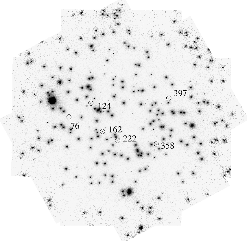
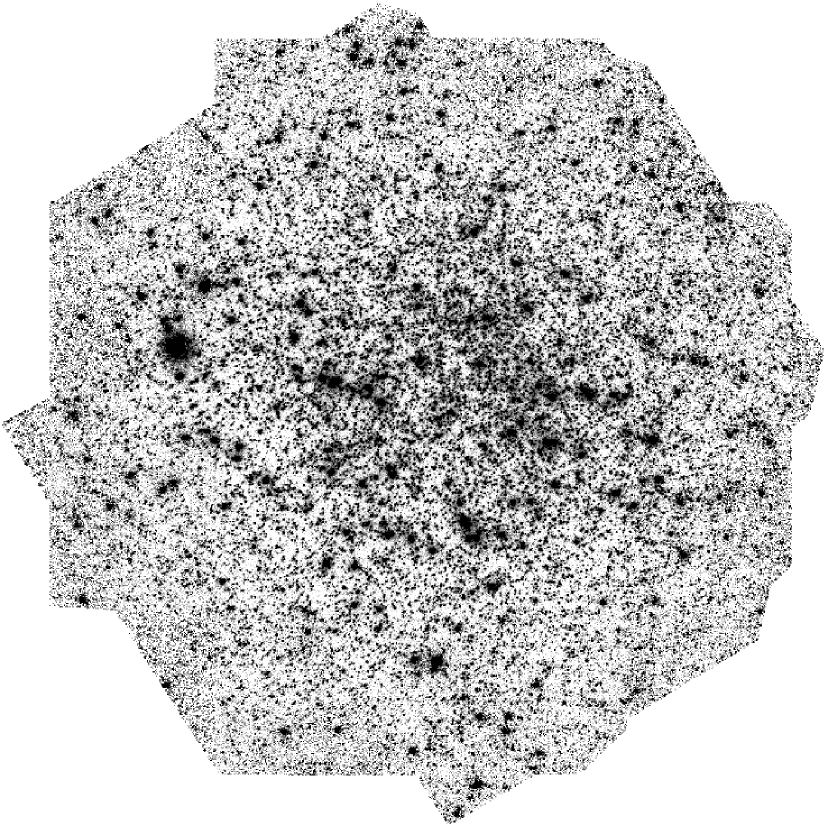
Figure 1: Left: Mosaic of all $FUV$ exposures taken from NGC 2808’s core. The single exposures were taken with slight offsets and rotation with respect to each other which led to the strange shape of the mosaic. Variable candidates are marked with black circles and their corresponding catalogue number in Table 1; see also Sect. 3.2. The images are displayed on a logarithmic intensity scale in order to bring out the fainter sources and illustrate the non-uniform background caused by the varying exposure times across the images. Right: Mosaic of all $NUV$ exposures of the same region of NGC 2808. Note the severe crowding in the $NUV$.

NGC 2808 was observed with the Space Telescope Imaging Spectrograph (STIS) on board the HST in January/February 2000. The original purpose of these observations was to provide geometric distortion corrections for the STIS camera. However, such calibration data are of course also of scientific interest, as already shown by Brown et al. (2001). Images were taken using the F25QTZ and F25CN270 filters, which are located in the far- and near-UV wavebands, with central wavelengths of 1590 Å ($FUV$, F25QTZ) and 2700 Å ($NUV$, F25CN270), respectively. The plate scale is $0\farcs 0248/\rm{pixel}$, resulting in a field of view of $25\arcsec\times 25\arcsec$ for both filters. The exposure times for the single exposures vary between 480 and 538 sec. The observations were positioned on the cluster centre; Fig. 1 shows the combined images. The mosaic images were constructed using MONTAGE 2 (Stetson, 1994), which registers all the image frames to a single reference frame - incorporating shift, scale, rotation, and distortions determined from positions of the brightest stars.

The resulting $FUV$ and $NUV$ mosaic images show a strange shape that is due to the small offsets and rotation of the single exposures with respect to each other. The diameter of the mosaics is $\approx 2100~{}\rm{pixel}$ or $\approx 52\arcsec$. Since the cluster’s core radius is $16\arcsec$, the complete core is covered by our mosaic images.

As can be seen immediately, the $NUV$ mosaic is extremely crowded. Crowding, on the other hand, is not a problem in the $FUV$ image. Note that the effective exposure times vary strongly across both mosaics. This is responsible for the increased background noise in the outskirts of the mosaics, where exposure times are low compared to the central regions (which have maximum exposure times of 8906 sec [$NUV$/F25CN270] and 8916 sec in the [$FUV$/F25QTZ]).

2.1 Source detection

As already mentioned in Sect. 1, we reinvestigate the same dataset studied by Brown et al. (2001), but with a different focus. Here, our main goal is to search for faint and/or variable $FUV$ sources (CVs, BSs, WDs). We therefore take special care to detect even weak sources in the $FUV$ images, which allows us to construct a very deep CMD.

As noted above, the exposure time is not uniform across the $FUV$ mosaic, which means that the outer parts of the image (with the lowest exposure times) have the noisiest background. In order to avoid both a large number of false detections in these regions (caused by noise peaks), and multiple detections in the halos of bright stars, we created a noise map which we used to “smooth” the image. As a first step, we then used the daofind routine of daophot (Stetson, 1991) running under iraf on the smoothed image to detect $FUV$ sources. We overplotted the resulting source coordinates on the $FUV$ mosaic and inspected them by eye. Overall, this source finding technique appeared to work well for bright sources (except for a few multiple detections around bright stars that we deleted by hand). However, it did not work as well for faint sources, especially in the deep, central part of the mosaic. Thus, we added a further 211 sources by hand. In total, our catalogue of $FUV$ sources contains 521 entries.

Source detection in the $NUV$ mosaic is a tedious task due to the severe crowding and depends critically on the daofind detection threshold. If the detection threshold is too high, no faint sources will be detected in the centre of the mosaic (which has maximum exposure time). The situation can be improved by lowering the detection threshold, but this also leads to false “detections” in the noisy outskirts. (The same is true for the $FUV$ mosaic, but less of a problem, since crowding is much less severe. We could therefore simply adopt a relatively high threshold in daofind and add the missing sources by hand.) However, it is important to realize that our goal is not to detect all $NUV$ sources, but to locate $NUV$ counterparts to our $FUV$ sources. In practice, we therefore chose to work with an intermediate threshold, designed to yield most of the detectable $NUV$ counterparts while keeping the number of false detections at bay. This is important, because if there are too many false detections, some will be matched erroneously to real $FUV$ sources.

In order to match the $FUV$ and $NUV$ catalogues, we first transformed the $NUV$ coordinates onto the frame of the $FUV$ mosaic. We then checked for common pairs within a tolerance of 1.5 pixels; this resulted in 306 matches. Careful inspection of the registered $NUV$ image around unmatched $FUV$ sources revealed an additional 50 $NUV$ counterparts within this tolerance that had not been detected by daofind. Increasing the tolerance to 2 pixels added another 23 matches. These additional matches are located mainly in the outskirts of the mosaic where our coordinate transformation is slightly less accurate, thus justifying an increased matching tolerance. All stars listed in Brown et al. (2001) were found in our $FUV$ catalogue; however, 25 of them did not have $NUV$ matches within 2 pixels. Closer inspection by eye revealed that these stars are either located in the outer regions of the mosaic and had probable $NUV$ counterparts outside the 2 pixel tolerance radius, or they had faint $NUV$ counterparts that are located in the most crowded inner area and were not initially detected by daofind. We therefore added these missing matches by hand.

A catalogue listing all of our $FUV$ sources is given in Table 1. We include sources without $NUV$ counterparts in Table 1, because these are likely to include additional WD and CV candidates. Among the sources with $NUV$ counterparts, we have marked all pairs that were matched with the higher tolerance of 2 pixel or were added by hand. In total, our catalogue contains 521 $FUV$ sources, including 403 with $NUV$ counterparts. All 295 sources listed in Brown et al. (2001) are also contained in our catalogue.

2.2 Aperture photometry

Aperture photometry was obtained using daophot (Stetson, 1991). Following Brown et al. (2001), we chose an aperture radius of 4 pixels and used an annulus between 4 and 10 pixel for sky subtraction. An exposure map was created that accounts for the different exposure times at different locations in the composite image. For the calibration to the STMAG-system we used the aperture corrections derived by Brown et al. (2001), namely 1.83 and PHOTFLAM of 1.11e-16 $\rm{erg}$ $\rm{s}^{-1}\rm{cm}^{2}\AA^{-1}/(\rm{counts}$ $\rm{s}^{-1})$ for the F25QTZ data, and 1.44 and PHOTFLAM of 3.92e-17 $\rm{erg}$ $\rm{s}^{-1}\rm{cm}^{2}\AA^{-1}/(\rm{counts}$ $\rm{s}^{-1})$ for the fluxes obtained with F25CN270.

The results of aperture photometry depend on the coordinates of the source that has to be measured, or, to be more precise, on the “centering”. Several re-centering algorithms are available under phot in daophot running under iraf. Brown et al. (2001) created their coordinate list by centering on each star by eye. We used their photometry as a point of reference, and hence adopted a Gaussian recentering algorithm, since this yielded the best agreement with their measurements. Fig. 2 displays the magnitude differences between our photometry and that of Brown et al. (2001), in both $FUV$ and $NUV$ bands. Overall, the agreement is very good, with a few notable exceptions discussed below.

For star no. 516 (Id. 29 in Brown et al., 2001) the difference between our photometry and Brown et al.’s (2001) is 0.6 mag in $FUV$. This star is located in the outer regions of the $FUV$ mosaic and appears somewhat elongated. This might be because the object is a blend of two sources, or because the PSF is smeared out since the coordinate transformations used to construct our mosaic are least reliable in the outermost regions of the image. The latter effect would be exacerbated by the asymmetric $FUV$ PSF and might cause the brightness to be underestimated when using a small aperture of only 4 pixels. The situation is similar for star no. 500 (Id. 13 in Brown et al. 2001), which is 0.45 mag fainter in our photometry, is also located close to the edges of the mosaic and appears somewhat elongated. However, a difference greater than 0.1 mag in the $FUV$ occurred only for 17 stars, and a difference greater than 0.15 mag only for 5 stars.

For the $NUV$, we found a magnitude difference of 0.985 mag for star no. 426 (Id. 189 in Brown et al. (2001)). This seems to be a case where Brown et al. (2001) matched a different $NUV$ source than we did. Though we are quite confident that we correctly matched most of the stars in $FUV$ and $NUV$, this discrepancy is a useful reminder that occasional mismatches might still occur due to the extreme crowding in the $NUV$ images. This is especially true for fainter sources, and mismatches probably contribute to the rising $NUV$ differences towards fainter magnitudes. However, differences greater than 0.15 mag occurred for only 18 stars in the $NUV$. Setting aside these extreme cases, the mean absolute differences between Brown et al.’s (2001) magnitudes and ours are $0.03\pm 0.03$ mag in $FUV$ and $0.03\pm 0.02$ mag in $NUV$. Thus, in general, there is good agreement between their catalogue and ours. The remaining differences can be explained by the different methods used to construct the mosaic images, to detect the sources, the different centering algorithms for the photometry and by the severe crowding in the $NUV$ images.

3 Results and Discussion

3.1 The FUV-NUV CMD

Fig. 3 shows the $FUV-NUV$ CMD of NGC 2808’s core region. Several distinct stellar populations can be seen, including blue HB stars, BSs, WDs, but also CV candidates. Our CMD reaches approximately 2 magnitudes deeper than that presented by Brown et al. (2001). This is because we took special care in detecting faint sources in the $FUV$ mosaic (Sect. 2.1). We also note that we plot all sources independent of their photometric errors, whereas Brown et al. (2001) only included sources satisfying $m<22$ mag and $\sigma_{m}<0.2$ mag in both $FUV$ and $NUV$. However, we stress that only 7 of the sources plotted have errors exceeding 0.2 mag in $FUV$, and all of these have errors in the range 0.2 - 0.3 mag. We therefore still regard these as significant detections.

To aid in the interpretation of the CMD, we have also calculated and plotted a set of theoretical tracks. In the following, we will first briefly describe the construction of the theoretical tracks and then discuss the various stellar populations within our CMD.

3.1.1 Synthetic Photometry

Since main sequence stars and red giants are too cool to show up in our CMD, we only present theoretical tracks for the zero-age horizontal branch (ZAHB), the zero-age main sequence (ZAMS) and the WD cooling curve in NGC 2808.

For our ZAHB track, we interpolated on the grid of oxygen-enhanced ZAHB models provided by Dorman (1992) to generate a set of models at the cluster metallicity of $\rm{[Fe/H]}=-1.36$. We then used synphot within iraf/stsdas to calculate the $FUV$ and $NUV$ magnitudes of stars on this sequence. This was achieved by interpolating on the Kurucz grid of model stellar atmospheres and folding the resulting synthetic spectra through the response of the appropriate filter+detector combinations.

The ZAMS is included because BSs are expected to lie near and slightly to the red of this sequence. In order to generate this track, we used the fitting formulae of Tout et al. (1996) to estimate the appropriate stellar parameters. The corresponding $FUV$ and $NUV$ colours were then again estimated from the Kurucz model grid within synphot.

Finally, our theoretical WD sequence was constructed by interpolating on the Wood (1995) grid of theoretical WD cooling curves, adopting a mean WD mass of 0.55 M_⊙. The models were then again translated to the observational plane by carrying out synthetic photometry with synphot, using a grid of synthetic DA WD spectra kindly provided by Boris Gänsicke (see Gänsicke, Beuermann & de Martino 1995).

For all our synthetic tracks we adopted a distance of 10.2 kpc and a reddening of $E_{B-V}=0.18\pm 0.01$ (Bedin et al., 2000).

3.1.2 HB stars

NGC 2808 is one of the most extreme examples among the globular clusters with unusual HB morphology, as first noted by Harris (1974). Since then this cluster has received considerable attention. In general, metallicity is regarded to be the first parameter that influences HB morphology. However, several globular clusters show different HB morphologies though their metallicities are similar (Rich et al., 1997). This led to the suggestion of a second parameter responsible for the unusual behaviour of the HBs in these clusters. Many parameters have been suggested (e.g. age, mass loss, stellar rotation etc.), but a thoroughly convincing explanation is still lacking (see e.g. Rood et al. 1993, Recio-Blanco et al. 2004). NGC 2808 shows a bimodal HB and one of the longest blue HB tails, the so-called extreme HB (EHB), with prominent gaps between the red HB (RHB), blue HB (BHB) and EHB (e.g. Clement & Hazen 1989, Ferraro et al. 1990, Byun & Lee 1991, Sosin et al. 1997, Walker 1999, Bedin et al. 2000). Only three other globular clusters are known that show bimodal HBs as well as gaps along their HBs, namely NGC 6229, NGC 6388, and NGC 6441 (Catelan et al., 1998). Sosin et al. (1997) discussed various mechanisms that might be responsible for the HB multimodality, none of which represents a satisfactory explanation. They suggested that a combination of effects might result in such a HB morphology, some of which might be unique to NGC 2808.

In our CMD, the two distinct clumps of bright stars around $FUV\sim 16$ mag correspond to the blue ($FUV-NUV\sim-0.7$ mag) and extreme ($FUV-NUV\sim-1.2$ mag) HB stars. The red HB stars are too cool to show up in the $FUV$ or $NUV$ images. As already reported by Brown et al. (2001), a gap within the EHB – as seen in optical CMDs for this cluster – is not evident in the $FUV-NUV$ CMD. Instead, the EHB clump is extended towards fainter magnitudes. Brown et al. (2001) suggested that these subluminous EHB stars (as well as the EHB gap in the optical CMDs) can be explained by a late helium-core flash that these stars undergo while they descend the WD sequence. The recent findings of Moehler et al. (2004) and Momany et al. (2004) generally support this theory. For a comprehensive analysis of the HB stars in the $FUV-NUV$ CMD, we refer the reader to Brown et al. (2001).

3.1.3 Blue stragglers

A trail of stars can be seen in Fig 3, starting from the BHB clump and reaching down below the theoretical ZAHB sequence towards the faint red corner of our CMD. These sources show magnitudes fainter than the ZAHB, but brighter than the ZAMS. The location of these objects agrees with the expected location of BSs, which are thought to be dynamically-formed objects resulting from a collision or coalescence of two or more MS stars. They are more massive than normal cluster MS stars and therefore we expect them to be already somewhat evolved. This explains their location slightly above and to the red of the ZAMS. We find 61 BS candidates, but caution that this should not be taken as a strict number since the various zones in our CMD partly overlap, and the discrimination between the CV and BS candidates, in particular, is difficult (see below).

3.1.4 White dwarfs

Fig. 3 reveals a population of 40 objects that lie near the theoretical cooling curve and are therefore probably hot, young WDs. Of these, 22 are brighter than $FUV=21$ and should be detectable across the full $FUV$ and $NUV$ mosaics. How many WDs should we expect to see? Following Knigge et al. (2002), we can obtain a simple estimate by scaling from the number of HB stars in the same field of view. We count $\approx 210$ BHB and EHB stars in our CMD, but, as noted above, RHB stars are too cool to show up. We therefore estimate the total number of HB stars by adopting the ratio of (RHB+BHB+EHB)/(BHB+EHB) $=1.86$ found by Sosin et al. (1997). We therefore expect a total of $\approx 390$ HB stars in our field of view. Given that the lifetime of stars on the HB is approximately $\tau_{HB}\simeq 10^{8}$ yrs (e.g. Dorman 1992), we can predict the number of WDs above a given temperature on the cooling curve from the relation

$\frac{N_{WD}}{N_{HB}}\sim\frac{\tau_{WD}}{\tau_{HB}}$

where $\tau_{WD}$ is the WD cooling age at that temperature (e.g. Knigge et al. 2002). WDs at $FUV\sim 21$ mag on our WD sequence have a temperature of $T_{eff}=38,000$ K and a corresponding cooling age of $\tau_{WD}\simeq 4\times 10^{6}$ yrs. We therefore predict a population of approximately 16 WDs brighter than $FUV=21$, which is in reasonable agreement with the observed number of 22. This strongly suggests that most of our candidates are indeed WDs.

3.1.5 CV candidates

Fig. 3 reveals quite a number of stars that are located between the WD and ZAMS tracks. This is a region in which we might expect to find CVs. We estimate that there are $\simeq 60$ sources in this “CV zone”. How does this number compare to theoretical predictions? We can attempt to answer this question by scaling the number of tidal capture CVs predicted for 47 Tuc to NGC 2808. To this end, we use the simplified estimate for the capture rate in globular cluster cores (Heinke et al., 2003)

$\Gamma\propto\rho_{c}^{1.5}\cdot r_{c}^{2}$,

where $\rho_{c}$ is the central luminosity density and $r_{c}$ the core radius. Based on this, we find that the total number of dynamically-formed CVs in NGC 2808 should be quite similar to 47 Tuc, in which Di Stefano & Rappaport (1994) predicted a population of $\sim 190$ active CVs formed via tidal capture. For 47 Tuc, Di Stefano & Rappaport (1994) found that approximately half of the captures would take place within 1 core radius. A CV formed outside the core will drift towards the centre due to mass segregation. Thus a given active CV should be found in the core today if its age exceeds the relaxation time-scale at the location where it formed. Given our detection limits, we cannot hope to detect the very oldest CVs, since these are also the faintest. In order to obtain a rough estimate, we will assume that we can detect most CVs whose secondaries have not yet been whittled down to brown dwarfs, but none of the latter. Thus our dividing line is between CVs whose orbital periods are still decreasing, and the so-called period bouncers, whose periods are lengthening (see Di Stefano & Rappaport, 1994, for details). Based on Fig. 2 in Di Stefano & Rappaport (1994), the oldest CVs we can detect will therefore have ages on the order of $10^{9}$ yrs. This is comparable to the relaxation time-scale at the half-mass radius of NGC 2808, so some, but probably not all dynamically-formed active CVs should have had time to reach the core. Given this ambiguity, we assume that between 50% and 100% of active CVs in NGC 2808 should be within our field of view. However, only about half of these are above our adopted detection limit, yielding a final prediction between $45-95$ CVs. We stress that this is an extremely rough estimate, but it does bracket the observed number of sources in our CV zone. Thus, a significant fraction of these candidates might indeed be CVs.

We caution that other sources might also occupy our CV zone. We have to consider the possibility that mismatches might have occurred, though special care has been taken in detecting and matching the $FUV$ and $NUV$ sources (see Sect. 2.1 and 2.2). Non-interacting WD/MS binaries without accretion would also lie in the CV zone. However, according to our ZAMS sequence, a turn-off star with a mass of 0.85 M_⊙ would have a $NUV$ magnitude of $\approx 23$. These objects would therefore be expected in the CV zone, but close to the WD cooling sequence where we find about 10 objects. If we do not consider these 10 sources, our number of CV candidates would be rendered to $\approx 50$, which is still consistent with our above estimates. In principle, our CMD may also contain background/foreground sources. However, we expect field star contamination to be negligible (see e.g. Ratnatunga & Bahcall 1985).

3.1.6 Cumulative distributions of the stellar populations

Fig. 4 shows the cumulative radial distributions of the stars that show up in our CMD. We distinguish between HB stars (dotted line), CV candidates (dot - short dashed line), WD candidates (long dashed line), and BS candidates (short dashed line). The top panel shows the distribution if all stars of the corresponding population are considered, independent of their magnitude. However, as pointed out in Sect. 2.1, the exposure time is not uniform across our mosaic, thus also the detection limit varies across the mosaic. For the outermost regions with the lowest exposure time all sources at least down to $FUV=21$ mag are detected. We try to avoid selection effects by adopting this as a limiting magnitude for our entire dataset. The lower panel in Fig. 4 shows the cumulative distributions of the magnitude-selected data.

The most striking differences seem to be between our HBs and WD candidates, which show the least central concentration, and the BSs and CV candidates, which appear to be the most centrally concentrated populations. This is in agreement with Walker (1999) and Bedin et al. (2000) who presented deep wide-field photometry and found no radial gradient in the distribution of the EHB stars. In order to compare the cumulative distributions and to establish the statistical significance of the differences between them, we applied a Kolmogorov-Smirnov test on the magnitude-selected dataset. However, we caution that the WD, CV and BS candidates cannot clearly be distinguished on the base of our CMD alone, i.e. we might have sources in one sample that actually belong to another one. Applying the magnitude selection to our data yields 22 WD, 30 BS, and 16 CV candidates. The HB stars are brighter than our selection criterion, and 209 of them are present in our field of view.

The K-S test returns the probability that the maximum difference between the two distributions being compared should be as large as observed, under the null hypothesis that the distributions are drawn from the same parent populations. According to this, the distributions of HBs and WDs are consistent with one another, with a K-S probability of 64.7 %. However, the distributions of BS and CV candidates differ significantly from those of the other two populations, with K-S test probabilities of 1.0 % (CVs vs HBs), 0.5 % (CVs vs WDs), 0.4 % (BS vs HBs) and 1.2 % (BSs vs WDs). The differences between the CV and BS distributions are not statistically significant, with a K-S probability of 49.3 % (CVs vs BSs).

The differences in the observed distributions might reflect the different masses of the various FUV populations. More specifically, CVs and BSs are expected to be considerably more massive than WDs and HBs, since CVs are WD/MS binaries and BSs are roughly speaking MS stars with masses above the cluster MS turn-off. The heavy CVs and BSs thus sink toward the cluster core and as a result are more centrally concentrated than the lighter WDs and HBs. Fig. 4 shows that the differences revealed by the K-S test are indeed in the expected direction.

On the other hand, CVs and BSs are believed to be objects formed through two- or three-body interactions such as tidal capture, collisions and mergers. These dynamical interactions take place preferentially in the dense cluster core. Thus, CVs and BSs may also be expected to be overabundant in the cluster core because this is their birthplace.

In either case, the enhanced central concentration of our CV candidates provides additional evidence that most of these sources are indeed CVs or non-interacting WD/MS binaries (as opposed to chance superpositions, foreground stars, etc), i.e. they either segregated towards the cluster centre, or they formed in the dense core region.

3.1.7 FUV sources with optical counterparts

Piotto et al. (2002) presented optical photometry for 74 Globular clusters, among them NGC 2808. The clusters were observed with HST/WFPC2 in the $F439W$ and $F555W$ bands, with the PC centred on each cluster’s centre. We searched for optical counterparts to our $FUV$ sources in their dataset, using xyxymatch within iraf. The transformation between the PC and STIS physical coordinate systems is tied to three HB stars as reference objects which could be clearly identified by eye in both the $F555W$ and the $FUV$ images. Following Knigge et al. (2002), we allowed for a maximum difference of 0.8 PC pixels (corresponding to 1.5 STIS pixels). In total, we found 97 counterparts to our $FUV$ sources. Out of these 9 are matches with MS stars, red giants or RHB stars. These stars are too cool to show up in our $FUV-NUV$ CMD, and thus these matches have to be explained otherwise: 13156 objects are present in the PC field-of-view in both optical bands, and the complete PC field is covered by our $FUV$ mosaic. In addition, 390 $FUV$ sources are located inside the area covered by the PC-data. Following the same statistical approach as in Knigge et al. (2002), we would expect up to 13 false matches. Thus, all the matches with MS stars and red giants can be explained statistically as false matches. The remaining 88 matches are all blue objects, either BHB or EHB or BS stars.

We marked all our $FUV$ sources for which we could find a blue optical counterpart as crosses in our $FUV-NUV$ CMD, and added their optical magnitudes and Id from Piotto et al. (2002) to our Table 1. As can be seen, one of our CV candidates, our star no. 170, does have an optical counterpart with $V=21.59$ mag and $B-V=-0.24$ mag. The blue optical colour of the counterpart (well off the cluster MS), and the quality of the $FUV$/optical match (the $FUV$ and optical positions agree to within 0.4 pixels) both suggest that the counterpart identification is secure.

3.2 Variability

As a first check for possible variability among our catalogue stars we performed photometry on all single $FUV$ images. For this purpose we first used the processed images that had been used to create the mosaic, i.e. these images were shifted and rotated to a common logical (i.e. image pixel) coordinate system. The great advantage is that we can use our coordinate list derived from the $FUV$ mosaic as an input to all of these processed images. The photometry was carried out in the same way as described above in Sect. 2.2. Of course only a fraction of our catalogue stars are present in each of the individual images, and for some stars we could obtain only one measurement.

Fig. 5 displays a plot of the mean magnitudes versus the corresponding $\sigma_{mean}$ calculated from all individual magnitudes derived for each star. As can be seen, some of our objects show a considerably higher $\sigma_{mean}$ than the majority. The crosses in Fig. 5 denote 28 objects that show a large $\sigma_{mean}$, compared to their companions with similar brightness, and that we chose to inspect more closely. We cross-checked our method using median (instead of mean) magnitudes and $\chi^{2}$ (instead of $\sigma_{mean}$). In each case the same stars show an excess $\sigma_{mean}$ (or $\chi^{2}$).

As a next step, we used the non-processed images to get more precise magnitudes for our 28 variable candidates. This is necessary, because the orientation of the PSF on these images is the same with respect to each image and not rotated as for the processed images that were used for creating the mosaic. Since these images now do not share a common logical coordinate system, we had to derive the coordinates for our variable candidates on each single image by using imexam under iraf. The photometry was carried out in the same way as described in Sect. 2.2.

Stars no. 79, 114, 175 and 269 of our Table 1 show very high $\sigma_{mean}$, however, these stars are located very close to bright stars, which makes it difficult to get accurate coordinates on the single images that have much shorter single exposure times than the mosaic. Consequently, these stars do not stand out as clearly as they do on the $FUV$ mosaic, and sometimes it is not possible to distinguish them from the halo of the nearby bright star. For 18 of the other stars that we selected on the basis of Fig. 5, the magnitude scatter either disappears when using the single non-processed image photometry, or too few measurements are available for reliable conclusions. However, for none of these 18 sources is a magnitude variation as evident as it is for star no. 358, see below. We note that Proffitt et al. (2003) compared observed and predicted count rates in the $FUV$ F25QTZ and found a much larger scatter between observations and predictions than expected from Poisson statistics. Only 6 stars out of the 28 candidates have more than 5 measurements and a $\sigma_{mean}$ well beyond the expected photometric scatter – also if we take the effect described by Proffitt et al. (2003) into account – and we consider these sources as “secure” variable candidates. The remaining 22 stars are labelled in Table 1 but are not discussed further here.

NGC 2808 was observed on only 4 days (18., 19. January 2000 and 16., 20. February 2000). This period is sufficient to search for signs of variability, but it is somewhat too short and too interrupted to present reliable lightcurves for our variable candidates. However, Fig. 6 shows the magnitudes versus time for the 6 sources that remain as good variable candidates after our analysis of the single, non-processed images, i.e. these stars still show a brightness variation that is well outside the expected magnitude scatter.

The 6 variable candidates are overplotted as diamonds in Fig. 3. Star no. 222 lies in the CV zone at $FUV-NUV=0.08$ mag, making it a good CV candidate. Star no. 397 is located close to the WD region in our CMD, but could certainly be a CV as well. As mentioned above, the WD and CV zones are likely to overlap and cannot clearly be distinguished on the base of our CMD alone.

The lightcurve for star no. 124 in Fig. 6 seems to suggest that this source might be an eclipsing binary, with the beginning of an eclipse indicated at the end of the first observing period. This star is located on our theoretical ZAMS. It is very likely that this star is a BS star, and some BS are known to be binaries (see Livio 1993, and references therein). Stars no. 162 and 76 are clearly located in the BS zone of our CMD. Their lightcurves, especially for star no. 162, seem to indicated that these stars are pulsating variables (for other examples of oscillating BSs, see Gilliland et al. 1998, and references therein).

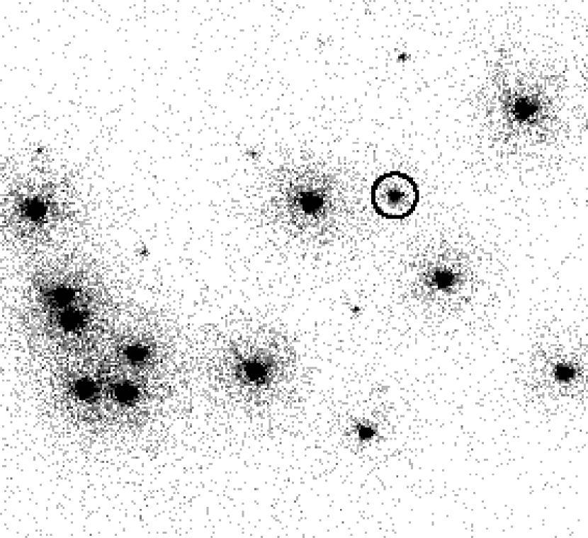
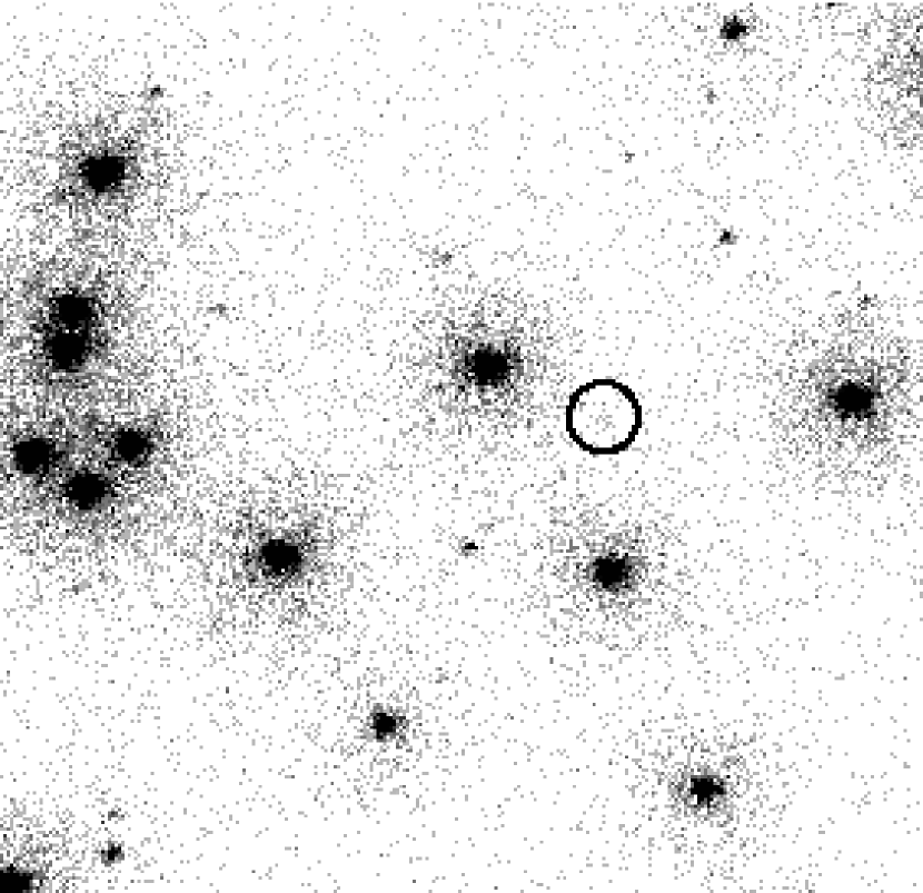
Figure 7: Left: Close up of image o60q02f6q centred on star no. 358 which clearly sticks out as one of the brighter objects ($FUV=18.212$ mag). Right: Close up of image o60q52kxq, centred around the same star, marked with a black circle in both figures. As can be seen, star no. 358 has practically vanished.

Star no. 358 is presented in the top panel in Fig. 6. This is the brightest of our variable candidates, located at $FUV=19.06$ mag and $FUV-NUV=1.58$ mag and thus above the BS zone. It has a $\sigma_{mean}=1.9$ mag in Fig. 5, and its brightness drops about 4 magnitudes from the January to the February observations. This can be seen by eye on the $FUV$ images, as illustrated in Fig. 7. The image on the left hand-side of this figure represents a close up of image o60q02f6q. Star no. 358 clearly sticks out as one of the brighter objects ($FUV=18.212$ mag). The image on the right hand-side of Fig. 7 is a close up of exposure o60q52kxq, centred around the same region. As can be seen, star no. 358 has practically vanished. We found that the coordinates of this star agree within $\approx 1\arcsec$ in $\delta$ with the RR Lyrae V 22 of Corwin et al. (2004). Downes et al. (2004) pointed out that the amplitude of RR Lyrae can be as high as 4 mag in the $FUV$. Also, the lightcurves of RR Lyrae are known to be asymmetric with a period of 0.1 to 0.3 days. It seems that we observe a brightness peak in the first observation period and a minimum in the second one. Recently, Wheatley et al. (2004) found $FUV$ variations of about 4.9 mag within the 0.56432 d period of their RR Lyrae star, which is of the same order as the $FUV$ amplitude we found for our star no. 358. Large $FUV$ amplitudes are to be expected since the amplitudes of the pulsations increase towards the far-ultraviolet (Downes et al., 2004; Wheatley et al., 2004). The UV photospheric flux is extremely sensitive to $T_{eff}$ in the temperature range of RR Lyrae stars ($T_{eff}\sim 6500$ K).

4 Summary

We have reanalyzed far-UV STIS HST observations of the core region of the globular cluster NGC 2808. These data were first analyzed by Brown et al. (2001) with an emphasis on the bright BHB and EHB stars, whereas our focus has been on the population of fainter $FUV$ sources. Taking special care in detecting the faint $FUV$ sources, we were able to present a $FUV-NUV$ CMD that is $\approx 2$ mag deeper than the one presented by Brown et al. (2001). The overall agreement between their photometry and ours is good.

Various stellar populations show up in our CMD, including the BHB and EHB stars for which this cluster is well known. RHB and MS stars are too cool to show up. However, approximately 60 BS candidates are present in our CMD. About 40 sources are located close to our theoretical WD cooling curve and are probably hot, young WDs. We estimated the number of WDs by scaling from the number of HB stars that are present in our field of view, and found that approximately 16 WDs can be expected at $FUV\leq 21$ mag. This is in reasonable agreement with the observed number of 22 at a completeness limit of 21 mag. Our CMD reveals a number of stars that are located in the CV region between the WD cooling curve and the ZAMS. Approximately 60 sources can be found in this region, but we caution that due to the photometric scatter the discrimination between the individual zones can be difficult. Using a simplified estimate for the capture rate in globular cluster cores (Heinke et al., 2003), we found that the number of dynamically-formed CVs in the core of NGC 2808 is comparable to 47 Tuc, and broadly consistent with the number of candidates we detected. This suggests that many of our candidates might indeed be CVs. The cumulative radial distributions of the individual stellar populations indicate that our BS and CV candidates are more centrally concentrated than HBs and the WD candidates. This may be a result of mass segregation, but might also reflect the fact that CVs and BS are mostly dynamically-formed populations that were preferentially born in the dense cluster core. We compared our $FUV$ data with optical HST/WFPC2 data presented by Piotto et al. (2002) and found 88 optical counterparts for our HB and BS stars and for one CV candidate (our star no. 170).

We searched for variability among our catalogue stars and found six good variable candidates. These stars are all located at $FUV\geq 19$ mag and distributed over the entire colour range of our CMD. Two variable candidates, stars no. 222 and 397, lie in the CV zone of our CMD and thus are excellent CV candidates. Stars no. 124, 162 and 76 are all located in the BS zone of our CMD. The lightcurve of star no. 124 suggests that this source may be an eclipsing binary, while the other two stars might be pulsating variables.

The most striking among our variable stars is our star no. 358 . This is the brightest variable in our sample and shows a considerable drop off about 4 mag during the observation period. We identified this star as the RR Lyrae V 22 in Corwin et al. (2004). RR Lyrae can show large $FUV$ amplitude variations of even up to $6-8$ mag (see Downes et al. 2004, Wheatley et al. 2004).

Overall, the results of our study confirm that $FUV$ observations are a powerful tool for studying hot, and especially dynamically-formed, stellar populations in the cores of GCs.

Figure 2: Lower panel: Difference in $FUV$ magnitude between our photometry and Brown et al.’s (2001). Only a few stars show differences greater than 0.1 mag, thus in general both datasets show good agreement. Upper panel: The same but for the $NUV$ magnitudes. See the text for a discussion of outliers.

Figure 3: $FUV-NUV$ CMD of the core region of NGC 2808. For orientation purposes, we include a theoretical WD cooling sequence, a zero-age main sequence, and a zero-age HB track (see text for details). The diamonds and the corresponding numbers denote variable $FUV$ sources, as discussed in Sect. 3.2. Mean errors for different $FUV$ magnitude ranges are given on the left-hand side of the CMD. The open circles with enclosed letters mark the positions of known field CVs if they were located at the distance and reddening of NGC 2808, the notation is the same as in Knigge et al. (2002). The crosses denote stars for which optical counterparts could be found in the Piotto et al. (2002) data. See the text for details.

Figure 4: Cumulative radial distributions of the stellar populations that show up in our CMD. Top panel: all sources that show up in the corresponding regions in our CMD are considered. Lower panel: only sources with $FUV\leq 21$ mag are considered. See the text for details.

Figure 5: Mean magnitudes versus $\sigma_{mean}$ derived from the individual photometries for each star.

Figure 6: Magnitudes versus time for 6 variable candidates. The diagrams have been interrupted for a better display of the magnitude variations in each observing period. The top panel shows the magnitude-time diagram for star no. 358. This star corresponds to the RR Lyrae V 22 (Corwin et al., 2004). It stands out much brighter in the images taken in the first observation interval, while it nearly disappears in the second one. See text for more details.

Table 1: Catalogue of all FUV-NUV sources. $\delta FUV$ and $\delta NUV$ denote the difference between our $FUV$, $NUV$ photometry and the one presented by Brown et al. (2001). Our $\alpha$ $\delta$ coordinates are based on the coordinate system given by the FITS-headers, but have been shifted to achieve the best match to the Brown et al. (2001) coordinates. This required offsets of $-0\farcs 13$ in $\alpha$ and $-0\farcs 6$ in $\delta$, after which the rms differences between our coordinates and Brown et al.’s (2001) are only $0\farcs 006$ in $\alpha$ and $0\farcs 048$ in $\delta$. However, as noted in Brown et al. (2001), although the relative astrometry is very accurate, the error in the absolute astrometry is much larger ($\approx 1\arcsec-2\arcsec$). Column 10 of our table lists the distance to the cluster centre which we determined from star number counts to be at $9^{\rm{h}}$ $12^{\rm m}$ $2.96^{\rm s}$ and $-64^{\circ}$ $51\arcmin$ $47.78\arcsec$. Only the first 20 sources are listed, the complete catalogue is available at CDS, Strasbourg.

no.	alpha	delta	$FUV$	$\Delta FUV$	$NUV$	$\Delta NUV$	$\delta FUV$	$\delta NUV$	radius	$\rm{Id}_{Brown}$	$\rm{Id}_{Piotto}$	$V$	$B$	comment
	[${}^{\rm{h}}~{}^{\rm m}~{}^{\rm s}$]	[${}^{\circ}~{}\arcmin~{}\arcsec$]	[mag]	[mag]	[mag]	[mag]	[mag]	[mag]	[$\arcsec$]			[mag]	[mag]
1	9 12 5.454	-64 51 26.761	20.808	0.170	22.187	0.229	-	-	26.51	-	-	-	-	a
2	9 12 5.313	-64 51 26.404	20.074	0.121	-	-	-	-	26.28	-	-	-	-
3	9 12 4.414	-64 51 25.250	21.729	0.260	19.842	0.062	-	-	24.54	-	-	-	-
4	9 12 5.149	-64 51 28.025	17.131	0.023	18.415	0.022	0.029	-0.025	24.34	253	-	-	-	pv
5	9 12 5.969	-64 51 30.908	22.210	0.229	23.169	0.379	-	-	25.69	-	-	-	-	pv
6	9 12 4.898	-64 51 27.503	21.911	0.198	-	-	-	-	23.92	-	-	-	-
7	9 12 6.306	-64 51 32.282	18.579	0.044	20.252	0.073	0.261	-0.152	26.50	289	-	-	-	n
8	9 12 5.210	-64 51 28.903	16.468	0.017	16.938	0.011	0.112	0.022	23.88	256	-	-	-	pv, e
9	9 12 6.131	-64 51 32.254	16.448	0.017	17.148	0.012	0.032	-0.088	25.63	287	-	-	-	e
10	9 12 5.059	-64 51 28.739	18.869	0.050	18.425	0.022	-0.019	-0.065	23.43	252	-	-	-
11	9 12 4.342	-64 51 26.459	16.422	0.023	17.003	0.016	0.108	-0.033	23.26	219	-	-	-	n, e
12	9 12 6.749	-64 51 34.589	16.458	0.023	-	-	-	-	27.63	-	-	-	-	e
13	9 12 4.119	-64 51 25.910	21.532	0.275	-	-	-	-	23.26	-	-	-	-
14	9 12 5.746	-64 51 31.458	20.506	0.105	19.294	0.033	-	-	24.27	-	-	-	-	pv
15	9 12 5.530	-64 51 30.936	19.978	0.082	17.486	0.014	-	-	23.65	-	-	-	-	pv
16	9 12 3.889	-64 51 25.800	19.452	0.091	-	-	-	-	22.96	-	-	-	-
17	9 12 3.460	-64 51 24.399	16.507	0.017	17.141	0.012	-0.057	-0.041	23.80	153	-	-	-	n, e
18	9 12 3.147	-64 51 23.712	16.475	0.023	17.072	0.016	-0.005	-0.032	24.31	128	-	-	-	a
19	9 12 3.336	-64 51 24.893	16.422	0.016	17.201	0.012	0.018	-0.071	23.20	145	-	-	-	n, e
20	9 12 5.822	-64 51 33.490	16.325	0.016	16.810	0.010	-0.025	-0.020	23.29	280	-	-	-

References

- Albrow et al. (2001) Albrow, M. D., Gilliland, R. L., Brown, T. M. et al. 2001, ApJ, 559, 1060
- Bedin et al. (2000) Bedin, L. R., Piotto, G., Zoccali, M. et al. 2000, A&A, 363, 159
- Brown et al. (2001) Brown, T.M., Sweigart, A.V., Lanz, T., Landsman, W.B., & Hubeny, I. 2001, ApJ, 562, 368
- Byun & Lee (1991) Byun, Y., & Lee, Y., 1991, in ASP Conf. Ser. 13: The formation and evolution of star clusters, p. 243
- Catelan et al. (1998) Catelan, M., Boressova, J., Sweigart, A. V., & Spassova, N. 1998, ApJ, 494, 265
- Clement & Hazen (1989) Clement, C. M., & Hazen, M. L. 1989, AJ, 97, 414
- Corwin et al. (2004) Corwin, T. M., Catelan, M., Borissova, J., & Smith, H. A. 2004, A&A, 421, 667
- Davies & Benz (1995) Davies, M. B., & Benz, W. 1995, MNRAS, 276, 887
- Davies (1997) Davies, M. B. 1997, MNRAS, 288, 117
- Di Stefano & Rappaport (1994) Di Stefano, R., & Rappaport, S. 1994, ApJ, 423, 274
- Dorman (1992) Dorman, B. 1992, ApJS, 81, 221
- Downes et al. (2004) Downes, R. A., Margon, B., Homer, L., & Anderson, S. F. 2004, AJ, 128, 2288
- Edmonds et al. (2003a) Edmonds, P. D., Gilliland, R. L., Heinke, C. O., & Grindlay, J. E. 2003a, ApJ, 596, 1177
- Edmonds et al. (2003b) Edmonds, P. D., Gilliland, R. L., Heinke, C. O., & Grindlay, J. E. 2003b, ApJ, 596, 1197
- Elson et al. (1987) Elson R, Hut P., & Inagaki S. 1987, ARA&A, 25, 565
- Fabian et al. (1975) Fabian, A. C., Pringle, J. E., & Rees, M. J. 1975, MNRAS, 172, 15P
- Ferraro et al. (1990) Ferraro, F. R., Fusi Pecci, F., Buonanno, R., & Alcaino, G. 1990, A&AS, 84, 59
- Gänsicke et al. (1995) Gänsicke, B., Beuermann K., & de Martino, D. 1995, A&A, 303, 127
- Grindlay et al. (2001) Grindlay, J. E., Heinke C., Edmonds, P. D., & Murray, S. S. 2001, Science , 292, 2290
- Gilliland et al. (1998) Gilliland, R. L., Bono, G., Edmonds, P. D. et al. 1998, ApJ, 507, 818
- Harris (1974) Harris, W. E. 1974, ApJ, 192, L161
- Harris (1996) Harris, W.E. 1996, AJ, 112, 1487
- Heinke et al. (2003) Heinke, C. O., Gindlay, J. E., Lugger, P. M. et al. 2003, ApJ, 598, 501
- Hut et al. (1992) Hut, P., McMillan, S., Goodman, J., Mateo, M., Phinney, E. S. et al. 1992, PASP, 104, 981
- Knigge et al. (2002) Knigge, C., Zurek, D. R., Shara, M. M., & Long, K. S. 2002, ApJ, 579, 752
- Knigge et al. (2003) Knigge, C., Zurek, D. R., Shara, M. M., Long, K. S., & Gilliland, R. L. 2003, ApJ, 599, 1320
- Livio (1993) Livio, M. 1993, ASP Conf. Ser. 53: Blue Stragglers, p. 3
- Moehler et al. (2004) Moehler, S., Sweigart, A. V., Landsman, W. B., Hammer, N. J. & Dreizler, S. 2004, A&A, 415, 313
- Momany et al. (2004) Momany, Y., Bedin, L. R., Cassisi, S. et al. 2004, A&A, 420, 605
- Piotto et al. (2002) Piotto, G., King, I. R., Djorgovski, S. G. et al. 2002, A&A, 391, 945
- Proffitt et al. (2003) Proffitt, C. R., Brown, T. M., Mobasher, B., & Davies, J. 2003, Instrument Science Report STIS 2003-01
- Ratnatunga & Bahcall (1985) Ratnatunga, K. U., & Bahcall, J. N. 1985, ApJS, 59, 63
- Recio-Blanco et al. (2004) Recio-Blanco, A., Piotto, G., Apapricio, A., & Renzini, A. 2004, A&A, 417, 597
- Rich et al. (1997) Rich, R. M., Sosin, C., Djorgovski, S. G. et al. 1997, ApJL, 484, 25
- Rood et al. (1993) Rood, R. T., Crocker, D. A., Fusi Pecci, F. et al. 1993, ASP Conf. Ser. 48: The globular cluster-galaxy connection, p. 218
- Sosin et al. (1997) Sosin, C., Dorman, B., Djorgovski, S., G. et al. 1997, ApJL, 480, 35
- Stetson (1991) Stetson, P. B. 1991, in 3rd ESO/ST-ECF Garching - Data Analysis Workshop, eds. Grosbøl P. J., Warmels R. H., p. 187
- Stetson (1994) Stetson, P. 1994, PASP, 106, 250
- Tout et al. (1996) Tout, C. A., Pols, O. R., Eggleton, P. P., & Han, Z. 1996, MNRAS, 281, 257
- Walker (1999) Walker, T. 1999, AJ, 118, 432
- Wheatley et al. (2004) Wheatley, J. M., Welsh, B. Y., Siegmund, O. H. W. et al. 2004, ApJ, 619, L123
- Wood (1995) Wood, M. A. 1995, Lecture Notes in Physics, 443, 41