A Near-Solar Metallicity, Nitrogen-Deficient Lyman Limit Absorber Associated with two S0 Galaxies

Abstract

The UV spectrum of the bright quasar PHL 1811 at $z_{\rm em}=0.192$ reveals a foreground gas system at $z=0.080923$ with $\log N({\rm H~{}I})=17.98\pm 0.05$. We have determined the abundances of various atomic species in this system from a spectrum covering the wavelength range 1160 to 1730 Å recorded at $7\,{\rm km~{}s}^{-1}$ resolution by the E140M grating of STIS on the Hubble Space Telescope (HST), supplemented by coverage at shorter wavelengths by the Far Ultraviolet Spectroscopic Explorer. The abundances of C II, Si II, S II and Fe II compared to that of O I indicate that a considerable fraction of the gas is in locations where the hydrogen is ionized. An oxygen abundance $[{\rm O/H}]=-0.19\pm 0.08$ in the H I-bearing gas indicates that the chemical enrichment of the gas is unusually high for an extragalactic QSO absorption system. However, this same material has an unusually low abundance of nitrogen, $[{\rm N/O}]<-0.59$, indicating that there may not have been enough time during this enrichment for secondary nitrogen to arise from low and intermediate mass stars. From the convergence of high Lyman series lines we can determine the velocity width of H I, and after correcting for turbulent broadening shown by the O I absorption feature, we derive a temperature $T=7070^{+3860}_{-4680}\,$K. We determine a lower bound for the electron density $n(e)>10^{-3}\,{\rm cm}^{-3}$ by modeling the ionization by the intergalactic radiation field and an upper bound $n(e)<0.07\,{\rm cm}^{-3}$ from the absence of much C II in an excited fine-structure level. The thermal pressure in the range $4<p/k<140\,{\rm cm}^{-3}\,$K could be confined by a warm-hot intergalactic medium (WHIM) structure with $\rho/\bar{\rho}\sim 20$ that might accompany a wall of galaxies at the same redshift, seen in data from the Sloan Digital Sky Survey. An $r$-band image of the field surrounding PHL 1811 recorded by the ACS instrument on HST shows that two galaxies at the same redshift as the gas are S0 galaxies, separated by only 34 and 87$h^{-1}_{70}\,$ kpc from the line of sight. One or both of these galaxies may be the source of the material in the Lyman limit system, which may have been expelled from them in a fast wind, by tidal stripping, or by ram-pressure stripping. Subtraction of the ACS point-spread function from the image of the QSO reveals the presence of a face-on spiral galaxy under the glare of the quasar; while it is possible that this galaxy may be responsible for the Lyman limit absorption, the exact alignment of the QSO with the center of the galaxy suggests that the spiral is the quasar host.

1 Introduction

The absorption lines detected in the spectra of background quasars allow us to examine in detail the nucleosynthetic products released to the gaseous media within and between galaxies (Lauroesch et al. 1996; Péroux et al. 2003; Pettini 2003; Prochaska 2004). This field of research has flourished over the last few years due to the availability of high-resolution spectrographs coupled to 8$-$10 m class ground-based telescopes. Elemental abundance patterns of absorbing gas clouds provide insights into the character and maturity of stellar systems associated with such absorbers, either through direct comparisons with abundances measured for old stars in our own Galaxy (Prochaska 2003) or theoretical models for chemical evolution (Matteucci, Molaro, & Vladilo 1997; Calura et al. 2004; Dessauges-Zavadsky et al. 2004). However, there remains a large scatter in abundances within the Damped Lyman Alpha (DLA) population at any given redshift, an outcome which has hampered efforts to synthesize a coherent picture of how heavy elements build up in the universe. For instance, recent studies have shown that low-redshift QSO absorbers have metallicities that range from substantially sub-solar abundances (Tripp et al. 2002, 2004) to nearly solar values (Prochaska et al. 2004). Some systems show significant nitrogen underabundances (Tripp et al. 2004) while other absorbers appear to have normal (solar) nitrogen abundances with respect to other metals (Savage et al. 2002). Nevertheless, there has been some progress in noting a general trend: by accumulating a large database of metallicity measurements from DLAs and averaging these values over broad redshift intervals, Prochaska, et al (2003) have found evidence for an increase in elemental abundances with increasing cosmic time. This finding is consistent with our expectation that the universe becomes more metal-rich as it evolves, but the wide range in observed abundances still indicates that absorption systems probably arise from gas residing within, or cast off from, a very heterogeneous population of galaxy types and ages. Clearly, more studies are needed to understand the chemical enrichment of low-z QSO absorbers, which will ultimately lead to a better understanding of chemical evolution over the past 10 Gyr in parts of the universe that have baryon densities that are well above average.

A considerable amount of effort has gone into trying to understand the nature of galaxies that may be associated with QSO absorption systems, but for high-$z$ systems whose abundances are obtained from ground-based telescopes, detailed investigations into the origin of the absorption are hampered by the great distances. That is, without the ability to study well resolved images of galaxies near quasar lines of sight, investigating the exact causes of the abundance fluctuations will inevitably prove extremely difficult. For example, variations could arise from QSO sightlines intercepting similar galaxies at different galactocentric radii; alternatively, differences may be a direct results of galaxy age, morphological type, star formation history, and/or gas dynamical processes.

Taken together, these arguments offer a compelling case for studying absorption systems at low redshift, where both individual galaxies and galactic large scale structure can be studied in detail. An additional need arises from the present undersampling of low-$z$ systems, which are more difficult to survey since the absorption lines required for abundance measurements lie in the ultraviolet (UV). Unfortunately, present-day UV spectrographs and space telescopes can observe only the very brightest quasars. As a result, an extrapolation to $z=0$ of the $N$(H I)-weighted metallicity trend at high-$z$ shown by Prochaska et al (2003) is highly uncertain because there are not enough observations of systems with $z<1.5$.

In this paper we report abundance measurements for one such low-redshift system, the $z=0.08$ Lyman limit absorber towards PHL 1811. We also assess the probable contributors (galaxies) that may be the origin of the absorption. The discovery of a gas system that produced continuous, nearly total absorption shortward of the Lyman limit in the spectrum of PHL 1811 arose from an initial, brief observation of the QSO using the Far Ultraviolet Spectroscopic Explorer (FUSE). In §2.1 we give some background on the discovery of the system and the limited findings we obtained from the early dataset, and in §2.2 we recount our initial investigations of the galaxies in the immediate vicinity of the quasar sightline that we found to have redshifts similar to that of the absorption system.

The traditional definition of a “Lyman Limit System” is one that has an H I column density high enough to cause absorption beyond the Lyman limit, but that is too low to show damping wings in the Ly$\alpha$ transition. A DLA was originally defined by Wolfe et al (Wolfe et al. 1986) to have $\log N$(H I)$\geq 20.3$, based on their ability to detect damped absorption in low resolution spectra with an equivalent width $\geq 10$ Å. In the case of the absorption towards PHL 1811 though, the high resolution used to record the Ly$\alpha$ transition enables us to detect a damping wing in the line (§4.1.1) that leads to an accurate determination of $N$(H I), slightly less than $10^{18}$ cm^-2. To be consistent with the accepted terminology for a system with this much neutral hydrogen, however, we will continue to describe this absorption system as a Lyman limit system.

Our abundance measurements came from an HST program, which used the medium resolution echelle grating (E140M) and Space Telescope Imaging Spectrograph (STIS) (§3.1). We have supplemented these data with more extensive observations from FUSE (§3.2), which provide data at improved S/N at the shortest wavelengths. We derive abundances of various species using different methods appropriate for each case at hand in the subsections of §4.1. From the convergence of Lyman series lines at the shortest wavelengths in the FUSE data, coupled with observations of O I in the STIS data, we can determine permissible temperatures for the H I-bearing material (§4.2). This information, coupled with a range for the electron density, [with an upper bound defined by the population of C II in an excited fine-structure level (§5.1) and a lower bound from a model for the photoionization of the material (§5.4)] help to define the physical characteristics of the system.

From our overview of our fundamental measurements of various atoms and ions in §5.2, we deduce that we are observing an absorber in which ionized gas dominates over neutral gas. For this reason, we have considered whether our elemental abundances have been distorted by our inability to see all stages of ionization. We investigate various ionization scenarios, including collisional ionization (§5.3), photoionization from the intergalactic radiation field for two values of the ionization parameter $U$ (§5.4), and a special case where the apparent abundances of N and O could in principle be altered by an intense stellar radiation field (§5.5) if stars that are invisible to us are indeed present inside this system. We caution that the level of technical detail within the last of these three subsections (§5.5 and supporting equilibrium equations given in the Appendix) is greater than that of the others, and the arguments are intended to defend our conclusions against the effects arising from a speculative extreme in ionization conditions; some readers may wish to skip this discussion.

As noted above, we are also interested in determining the origin of the Lyman limit system towards PHL 1811, and associating the results from our absorption line measurements with the galaxies and galactic large scale structure in the immediate vicinity of the quasar sightline. A small part of our HST observing program (one orbit) was devoted to obtaining an $r$-band image of the field around PHL 1811 using the Advanced Camera for Surveys (ACS) (§6.1); our goal was to apply standard surface photometry metrics (§6.2) to determine the morphology of the two galaxies close to the sightline that have redshifts similar to that of the Lyman limit system. We also wished to search for bars, spiral-arm patterns, or indicators of interesting dynamical phenomena in or near the galaxies, by enhancing the high-frequency image information in the data (§6.3). The results from these analyses for each galaxy are given in §7.1 and §7.2. Even though we did not use the coronagraphic mode of STIS to block light from the quasar, we were nevertheless able to subtract off a substantial part of the image flare from the QSO (§6.4) to reveal a loosely wound spiral arm pattern exactly centered at the position of the quasar (§7.3). However we are uncertain if this is the galaxy that is responsible for the Lyman limit absorption or is simply the host galaxy of the quasar.

Beyond the immediate area around the quasar sightline, we present in §8 evidence from the Sloan Digital Sky Survey (SDSS) that the Lyman limit system is within (or near the end of) a large-scale filament (or sheet) of galaxies at a similar redshift. We close with a discussion on how the abundance pattern in the absorber might be related to the chemical evolution of the gas (§9.1), speculate on the possible origins of the material (§9.2) and present a general summary of our results (§10).

2 Previous Findings and the Motivation for New Observations

2.1 Survey of Absorption Systems using FUSE

The research discussed here was triggered when Jenkins et al. (2003; hereafter Paper I) used FUSE (Moos et al. 2000; Sahnow et al. 2000) to perform an exploratory study of the Galactic and intergalactic absorption lines appearing in the spectrum of the extraordinarily bright quasar PHL 1811 at $z_{\rm em}=0.192$ (Leighly et al. 2001). We identified 7 extragalactic gas systems, one of which was a Lyman limit system at $z=0.08093$. Three of the systems have redshifts that differ by less than $2500\,{\rm km~{}s}^{-1}$ from that of the Lyman limit system. In Paper 1 we reported on the unusually favorable opportunity for research on intergalactic systems at low redshift: this quasar, the second brightest in the sky, shows twice the expected number of absorption systems over a path $\Delta z=0.192$ in the local universe. Moreover, there was only a 6% chance of seeing a Lyman limit system. Incidental information about PHL 1811 is given in Table 1 of Paper I.

The FUSE spectrum was of great value in providing a general picture of what absorption systems were present, but it had several drawbacks that made it difficult to derive quantitative results: (1) A large part of the spectrum contained many Galactic H₂ features, and chance overlaps with them, together with atomic features from the Galaxy and the other redshifted systems, blocked many lines of interest, (2) the wavelength resolving power of only $\lambda/\Delta\lambda\lesssim 20,000$ and the modest signal-to-noise ratio (maximum S/N was 22 per resolution element) generally led to the detection of only the strongest, most saturated lines and (3) various useful Lyman series lines (Ly$\beta$ and higher) in the Lyman limit system were on the flat portion of the curve of growth, which, along with a limit for the transmission below the Lyman limit, resulted in 2 orders of magnitude uncertainty in $N$(H I). Hence, only rudimentary information on element abundances and degrees of ionization could be obtained. Clearly, better spectra were needed to reach meaningful conclusions on the nature of gas within the Lyman limit system. A subsequent observing program using STIS in a moderate resolution echelle mode (E140M) provided such a spectrum. These data, combined with new, longer exposure FUSE observations intended to improve upon the S/N of the original spectra, now enable us to derive more precise measurements of absorption lines in the spectrum of PHL 1811.

2.2 Locations of Nearby Galaxies

In addition to using FUSE to observe the far-UV spectrum of PHL 1811, we presented in Paper I an $R$-band image of the $7\farcm 6\times 7\farcm 6$ field surrounding the quasar. We also measured the redshifts of seven of the galaxies in the field. Two of the galaxies, which we designated as G158 and G169, had redshifts close to that of the Lyman limit system. Their separations on the sky were $23\arcsec$ and $59\arcsec$ from PHL 1811, respectively, corresponding to transverse distances $\rho$ of 34 and 87$h^{-1}_{70}\,$ kpc. The images of the galaxies were not good enough to obtain definitive morphological classifications. Since we felt that it was important to learn more about these galaxies, we used the ACS on board HST to register images of the galaxies in greater detail. These observations are discussed in §6.

3 New Spectroscopic Observations

3.1 STIS

PHL 1811 was observed for 33.9 ks (13 HST orbits) with STIS (Kimble et al. 1998; Woodgate et al. 1998) using the E140M grating and the $0.2\times 0.06$ arcsec entrance aperture under a Cycle 11 HST observing program (ID = 9418). The observing time was distributed between two sessions; one was held on 2002 October 7 and 9, while the other was on 2003 July 8 and 9. The resolving power of the spectrum was $\lambda/\Delta\lambda=46,000$ [$\Delta v=7\,{\rm km~{}s}^{-1}$ (Kim Quijano et al. 2003)], and we obtained continuous coverage from about 1160 Å to 1730 Å, except for only 5 small gaps longward of 1634 Å caused by incomplete coverage of the echelle grating’s free spectral range by the MAMA detector. The signal-to-noise ratio in each resolution element (2 pixels) increased in an approximately linear fashion from 10 to 16 over the interval 1160 Å to 1250 Å, remained at 16 from 1250 Å to 1470 Å, and then it decreased linearly to 7 from 1470 Å to 1730 Å. The spectra were reduced and combined in the manner described by Tripp et al. (2001).

3.2 FUSE

In addition to the original observations reported in Paper I, new observations totaling 65.8 ks of integration time were made on 2 and 3 June 2003. All FUSE spectra were reduced using CALFUSE Version 2.2.2 and combined in the manner described in Paper I. The higher S/N FUSE spectrum provided more accurate equivalent widths for key lines belonging to the Lyman limit system. Also, high members of the Lyman series were recorded with better accuracy.

4 Analysis of the Spectra

4.1 Equivalent Widths and Column Densities

Table 1 lists the equivalent widths of absorption features associated with the Lyman limit system. The definitions of continua and their uncertainties followed from the methods outlined in the appendix of a paper by Sembach & Savage (1992). Errors in the equivalent widths represent the combined effects of noise in the lines and uncertainties in the continuum levels (the two were combined in quadrature to obtain the final error). Some of the measurements give results that are less than or about equal to their errors, but they are listed since they establish interesting limits to the column densities. In Figure 1 we show selected features of various heavy elements on a common velocity scale. Lines for different species warranted different methods of interpretation. In the following subsections, we outline the basic approaches for deriving the column densities shown in Table 1 (see also endnote $e$ in the table for brief statements on these methods).

4.1.1 H I

As discussed earlier in §2.1, the FUSE recordings of the high members of the Lyman series and the Lyman limit absorption gave very poor constraints on $N({\rm H~{}I})$. In Figure 2 we present the Ly$\alpha$ line at $z=0.080923$ from the new STIS spectrum. As expected, this line is strongly saturated. However, the right-hand side of the profile shows a well developed damping wing, from which we can measure a precise H I column density. As we discuss later in §5.5, we expect O I to be the most reliable tracer of the H I-bearing material. For this reason, we use the center of the 1302 Å O I feature to give the velocity zero point for most of the neutral hydrogen. We also observe that the maximum extent of the O I feature visible in Fig. 1 is only $40\,{\rm km~{}s}^{-1}$, which is small compared to the width of the Ly$\alpha$ feature. From this we conclude that most of the hydrogen is creating a damped profile that matches either of the two smooth absorption curves (drawn for two extreme choices of continua) shown in Fig. 2. Some remaining material, an amount too small to show up in the other atomic features, arises over a velocity range $-170$ to $-50\,{\rm km~{}s}^{-1}$.

Table 1: Equivalent Widths and Column Densities

	Observed	Transition		$W_{\rm r}\pm 1\sigma$ Error	$\log N\pm 1\sigma$ Error	Analysis
Species	$\lambda$ (Å)	$\lambda$ (Å)	$\log f\lambda$	(mÅ)	(${\rm cm}^{-2}$)	Method
H I	1314.046 (S)	1215.670	2.704	883$\pm 14$	$17.98\pm 0.05$	1
C II	1120.200 (F)	1036.337	2.088	95.3$\pm 5.7$	$\gg 14.70$	2
	1442.527 (S)	1334.532	2.234	147.8$\pm 3.8$
	1442.037 (S)			20.1$\pm 3.7$	$13.00^{+0.07}_{-0.09}$	3
C II∗	1120.937 (F)	1037.018	2.088	$-9.9\pm 7.9$	$<12.37$	3,4,5
	1443.797 (S)	1335.708	2.188	$-7.4\pm 6.4$
C III	1056.083 (F)	977.020	2.869	264.4$\pm 7.6$	$\gg 13.50$	6
C IV	1673.480 (S)	1548.195	2.468	121.8$\pm 10.9$	$13.90^{+0.51}_{-0.20}$	7
	1676.263 (S)	1550.770	2.167	90.8$\pm 9.9$
N I	1296.621 (S)	1199.550	2.199	3.4$\pm 5.8$	$12.44^{+0.30}_{-\infty}$	3,4
	1297.349 (S)	1200.223	2.018	5.4$\pm 5.7$
	1297.875 (S)	1200.710	1.715	0.2$\pm 5.8$
N II	1171.714 (S)	1083.994	2.079	85.6$\pm 10.3$	$13.92^{+0.49}_{-0.41}$	8
	string(F)			86.7$\pm 8.6$
O I	1050.351 (F)	971.738	1.128	21.9$\pm 13.1\tablenotemark{k}$	$\cdots$
	1055.443 (F)	976.448	0.509	0.7$\pm 6.9$	$<14.54$	3,5
	1068.788 (F)	988.773	1.773	66.1$\pm 9.8$	$\cdots$
	1123.328 (F)	1039.230	0.974	16.6$\pm 4.4$	$14.32^{+0.12}_{-0.17}$	9
	1407.544 (S)	1302.169	1.796	112.2$\pm 4.2$	$14.52^{+0.06}_{-0.04}$	10
Si II	1286.748 (S)	1190.416	2.541	79.0$\pm 3.1$	$13.95^{+0.05}_{-0.03}$	11
	1289.854 (S)	1193.290	2.842	94.2$\pm 3.3$
	1409.924 (S)	1304.370	2.052	62.9$\pm 4.9$
	1650.252 (S)	1526.707	2.307	102.3$\pm 10.8$
Si IV	1506.547 (S)	1393.760	2.854	108.1$\pm 5.9$	$13.53^{+0.23}_{-0.37}$	7
	1516.289 (S)	1402.773	2.552	81.7$\pm 5.4$
S II	1355.263 (S)	1253.805	1.136	6.7$\pm 5.5$	$13.70^{+0.16}_{-0.25}$	3,4
	1361.438 (S)	1259.518	1.320	12.6$\pm 6.6$
S III	1094.436 (F)	1012.501	1.647	35.7$\pm 8.0$	$\cdots$
	1286.505 (S)	1190.191	1.449	36.2$\pm 3.8$	$14.19\pm 0.06$	12
Ar I	1133.045 (F)	1048.220	2.440	$-1.9\pm 7.8$	$<12.60$	3,5
Fe II	1235.736 (S)	1143.226	1.342	10.0$\pm 6.0$	$\cdots$
	1237.586 (S)	1144.938	1.978	28.9$\pm 4.1$	$13.59^{+0.14}_{-0.12}$	7
	2810.586 (S)	2600.172	2.793	172$\pm 24$

Figure 1: Absorption features in the Lyman limit system at $z=0.080923$ in the STIS E140M spectrum of PHL 1811. The feature at $-102\,{\rm km~{}s}^{-1}$ for C II may not be real; see endnote $f$ in Table 1.

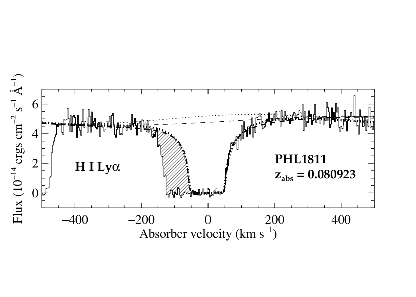
Figure 2: Ly$\alpha$ absorption for the Lyman limit system at $z=0.080923$ in the STIS E140M spectrum of PHL 1811. The velocity zero point is defined by the centroid of the apparent optical depth $\tau_{\rm a}$ of the feature belonging to the 1302 Å transition of O I (see Fig. 4). Two possible continua are shown by thin dotted and dashed lines, and their best-fit Voigt profile counterparts are shown with thick dotted and dashed lines. The two derived values of $N$(H I) differ from each other by 0.035 dex. The shaded portion shows the absorption by a small amount of extra hydrogen at velocities well outside the extent of the absorptions by heavier species shown in Fig. 1.

An optimum Voigt profile fit to the right-hand portion of the Ly$\alpha$ profile was obtained using a fitting procedure created by Fitzpatrick & Spitzer (1997). Our best value for $\log N({\rm H~{}I})$ is 17.98. A significant source of uncertainty in the fit is the choice of the continuum level. The two choices shown in Fig. 2 give values of $N$(H I) that indicate a (roughly 2$\sigma$) uncertainty of $\pm 0.035\,$dex. This uncertainty combined with the formal uncertainty found by the fitting program results in a net uncertainty of $\pm 0.05\,$dex at the 1$\sigma$ level.

4.1.2 O I

The O I feature recorded at the highest S/N and resolution was the 1302.17 Å transition observed at 1407.54 Å in the STIS E140M spectrum. The integral of the apparent optical depth $\tau_{\rm a}$ over the complete profile, $\int\ln[I_{\rm cont.}/I(v)]dv$, multiplied by the factor $10^{14.576}/f\lambda$ yields $N({\rm O~{}I})=10^{14.52}{\rm cm}^{-2}$. This value is higher than another determination $N({\rm O~{}I})=10^{14.32}{\rm cm}^{-2}$ based on a measurement of a rest-frame equivalent width $W_{\rm r}=16.6\pm 4.4\,$mÅ for the 1039.23 Å transition. The line is not resolved by FUSE, so we had to assume that it has a shape for its optical depth that is similar to the one shown at 1302 Å (see Fig. 4 in §4.2). The most error-prone portion of the 1302 Å profile is the part where the absorption is very deep, reaching a minimum intensity over a span of 3 pixels of about 0.06 times the local continuum (see Fig. 1). If we reduce the assumed strength of the absorption at this intensity trough enough to arrive at an intermediate $\log N({\rm O~{}I})=14.47$ for the entire profile, the $\chi^{2}$ increases by 1.6 above the minimum value (for $\log N({\rm O~{}I})=14.52$). For this case, we find that a reconstruction of $\int\tau_{\rm a}(v)dv$ for the 1039 Å transition should give $W_{\rm r}=22.2\,$mÅ, which is only $1.3\sigma$ above the measured value. Thus $\log N({\rm O~{}I})=14.47$ represents the best compromise between the two measurements, and its uncertainty is about 0.05 dex.

The measurement $W_{\rm r}/\lambda$ for the group of three lines near 988.8 Å is nearly the same as that for the 1302 Å transition, which has a value of $f\lambda$ that is about equal to the sum of the $f\lambda$ values for the three lines. Likewise, the upper limit for the strength of the 976.4 Å line and the measurement of three transitions at 971.738 Å yield results that are consistent with our adopted column density (the error in $W_{\rm r}$ for the latter is large because nearby strong lines prevent us from accurately measuring the continuum level). Generally, these lines support our conclusions based on the 1039 and 1302 Å lines, but with lower accuracy.

4.1.3 Si II

Of all the species for which we have absorption line data, the information for Si II is the most extensive. Four features were observed whose transition strengths span a factor of 6 and whose level of saturation range from moderate to strong. (The $\lambda 1260.422$ transition is apparently blended with another strong line that might be a Ly$\alpha$ forest line.) Under these circumstances, one can in principle derive a column density by modeling the observed result in terms of an instrumentally smoothed Voigt profile, with one or more velocity components. A simpler procedure that does not rely on a specific adopted model is to integrate the apparent optical depth $\tau_{\rm a}(v)$ over velocity $v$, (as we did for O I in §4.1.2 above), but correct for the possible under-representation of the (smoothed) opacities caused by unresolved, saturated structures within the profile using the method of Jenkins (1996). A generalization of this method beyond the analysis of two transitions involves finding at each velocity $v$ the best-fit curve of growth to the four values of $\tau_{\rm a}(v)$ as a function of $f\lambda$. The integral over velocity of the optical depths that are corrected for saturation yields $\log N({\rm Si~{}II})=13.95^{+0.05}_{-0.03}$.

4.1.4 N II

From our determinations of $N$(O I) and $N$(Si II) discussed above, we conclude that [Si II/O I]$\equiv$ $\log N({\rm Si~{}II})-\log N({\rm O~{}I})-\log({\rm Si/O})_{\odot}=+0.63$ (henceforth, we will adopt a notation [$A_{i}/B_{j}$], i.e., an extension of the standard bracket notation [$A/B$] for total element abundances, to denote the difference between the logarithm of the ratio of element $A$ in ionization state $i$ to element $B$ in state $j$ compared to the logarithm of the ratio of the elements’ solar abundances $\log(A/B)_{\odot}$). This apparently enormous enhancement of Si over O, compared to their solar abundance ratio, suggests that most of the Si II resides in a region containing fully (or mostly) ionized hydrogen, where there should be very little O I. Such a region will also hold most of the N II. For this reason, the velocity structure of the N II profile is expected to be very similar to that of Si II.

There is an unfortunate coincidence between the location of the $\lambda 1084$ N II line and that of a probable O VI $\lambda 1032$ line at $z=0.13541$ (see Paper I). We have measured the strength of the $\lambda 1038$ O VI line for this system and obtained marginal detections ($W_{\rm r}=14.0\pm 12.6\,$mÅ in the STIS spectrum and $W_{\rm r}=16.8\pm 10.8\,$mÅ in the FUSE spectrum). Combining the two and assuming the $\lambda 1032$ line is twice as strong as the $\lambda 1038$ one that we measured, we find an expected $W_{\rm r}(1032)=31.2\pm 16.4\,$mÅ. If we assume that the equivalent widths of the N II and O VI lines simply add to each other (which may not be entirely correct if the lines are actually very deep and overlapping), we find that the difference between the two, $W_{\rm r}=55.0\pm 17.7\,$mÅ, represents our best determination of the strength of the Lyman limit system’s N II absorption strength after allowing for the possible contamination by the O VI absorption feature from the other system.

Our nominal value for the strength of the $\lambda 1084$ line expressed in terms of $W_{\lambda}/\lambda$ is about equal to that of the Si II line at 1304 Å. Hence, if we assume that N II saturates in the same fashion as Si II (see above), $\log N({\rm N~{}II})=\log N({\rm Si~{}II})+\log(f\lambda)_{1304}-\log(f\lambda)_{1084}=13.92$. Likewise, this line’s $1\sigma$ upper limit for $W_{\rm r}$ translated into $W_{\lambda}/\lambda$ is about the same as that for the $\lambda 1190$ Si II line, which leads to $\log N({\rm N~{}II})=14.41$ by the same argument. The lower limit for $W_{\rm r}$ is substantially weaker than the $\lambda 1304$ Si II line; if we make the conservative assumption that it is unsaturated and $N$ scales linearly with $W_{\rm r}$ (see §4.1.8), we derive $\log N({\rm N~{}II})=13.51$. (A similar line of reasoning was applied to derive the $2\sigma$ error limits shown later in Figure 14.)

4.1.5 Nearly Saturated Doublets: C IV and Si IV

The doublets of C IV and Si IV both exhibit moderately strong saturation: the ratio of the line strengths for each species is $\gtrsim 1.3$, which is less than the expected 2.0 for these lines if they were unsaturated. We used the standard doublet ratio method (Strömgren 1948) to derive the column densities. This method was chosen so that we could implement a simple, yet reasonably conservative method of estimating the errors in the column densities. In each case, for $1\sigma$ upper and lower bounds we repeated the analysis using $W_{\rm r}({\rm weak})+1\sigma$ and $W_{\rm r}({\rm strong})-1\sigma$ for the former and $W_{\rm r}({\rm weak})-1\sigma$ and $W_{\rm r}({\rm strong})+1\sigma$ for the latter. We feel that the conservatism of adopting the worst combinations of equivalent widths for the limits is balanced by the shortcomings of the not so certain assumption that a doublet ratio analysis gives precise answers. Both species exhibit a best value for $b$ equal to $9\,{\rm km~{}s}^{-1}$, but they are offset from the lower ions by $+7\,{\rm km~{}s}^{-1}$.

In addition to the main feature of C IV, there is a broad, shallow component centered at about $v=-50\,{\rm km~{}s}^{-1}$. Traces of neutral hydrogen associated with this material may explain the presence of absorption to the left of the Ly$\alpha$ Voigt profile depicted in Fig. 2.

4.1.6 S III, C III and O VI

The two S III lines ($\lambda 1012$ and $\lambda 1190$) have intrinsic line strengths that differ by only 0.2 dex, and the relative error in the equivalent width of the former of the two is large. For these reasons, we felt that an application of the doublet ratio analysis was not appropriate. Instead, we noted that the radial velocity of S III is similar to those of C IV and Si IV (see Fig. 1), so we derived $N$(S III) from $W_{\rm r}$ of the $\lambda 1190$ line recorded by STIS under the assumption that $b=9\,{\rm km~{}s}^{-1}$ from the C IV and Si IV doublet ratio analyses.

The single available line of C III at 977.02 Å is very strong and is almost certain to be so badly saturated that we can only derive a lower limit that is probably far below the true value. As with S III, we assumed that the velocity structure of C III approximates that of C IV and Si IV (i.e., $b=9\,{\rm km~{}s}^{-1}$), but our extreme lower limit was based on $\tau_{0}=4$ (which, with the assumed value for $b$, would only produce a line with $W_{\rm r}=77\,$mÅ if the velocity profile were a pure Gaussian).

In Paper I we identified a feature that was likely to be caused by O VI $\lambda 1032$ absorption, but with a velocity displacement of $+110\,{\rm km~{}s}^{-1}$ with respect to the low ionization species. We were not able to confirm this identification by observing the $\lambda 1037$ feature because it is coincident with the Galactic Fe II line at 1121.97 Å. Another unfortunate coincidence is that the redshifted O VI $\lambda 1032$ line has a wavelength nearly the same as that of the Lyman 0$-$0 P(3) feature from Galactic H₂. However, we rejected this H₂ line as the principal source of this absorption because it was slightly stronger than the Lyman 1$-$0 P(3) line whose transition strength should be 3.3 times as large. Our improved S/N for the new FUSE spectrum warrants a reinvestigation of this issue. This time, we find that the 0$-$0 P(3) line has $W_{\rm r}=50.7\pm 7.0\,$mÅ (previously reported as $78\pm 16\,$mÅ) and the 1$-$0 P(3) line gives $W_{\rm r}=71.3\pm 7.4\,$mÅ (previously reported as $63\pm 11\,$mÅ). This inversion of the relative strengths of the two H₂ lines now makes it more reasonable to assert that the line is actually from Galactic H₂ instead of O VI at a redshift near that of the Lyman limit system. Moreover, the new spectrum shows the line to be narrow, again favoring H₂ as the origin rather than O VI. Finally, the Fe II line that would have blocked (or enhanced) the O VI $\lambda 1037$ line now seems to have about the right strength in relation to other Fe II lines with similar transition probabilities. Had there been an O VI feature at the same wavelength, one would expect this line to appear anomalously strong relative to the other Fe II lines. Thus, we withdraw our previous interpretation that the feature that appears at 1115.85 Å in the FUSE spectrum arises from O VI.

4.1.7 Fe II

A doublet ratio analysis based on the $\lambda 1145$ and $\lambda 2600$ lines indicates the saturation of the former is not large ($\tau_{0}=0.80$ for the nominal column density, 0.44 for the lower limit, and 1.49 for the upper limit, when derived using the prescription given in §4.1.5). The $\lambda 1143$ line of Fe II is too weak for a useful determination of $N$(Fe II), but its strength is consistent with what we would expect. Unfortunately, the $\lambda 1608$ line of Fe II is just beyond our STIS wavelength coverage.

4.1.8 Very Weak or Undetected Lines: C II^∗, N I, S II and Ar I

The lines of N I and S II are so weak that it is safe to assume that the derived values of $N$ are directly proportional to the equivalent widths. Hence $N=1.13\times 10^{20}(W_{\lambda}/\lambda)/(f\lambda)\,{\rm cm}^{-2}$ for these features. There is some small gain in considering all of the useful lines of a given case instead of just the strongest one. Thus, for these two species we evaluated the column densities $N_{i}$ and their respective errors $\sigma(N_{i})$ for the individual line measurements and then averaged the $N_{i}$ with weights proportional to $\sigma(N_{i})^{-2}$, yielding a combined result with an overall error equal to $(\sum\sigma(N_{i})^{-2})^{-0.5}$.

Neither C II^∗ nor Ar I lines are visible in the spectra. For Ar I, the $\lambda 1066$ transition is so much weaker than the $\lambda 1048$ one that it is of little value to consider it when the stronger line is not seen. The measurements of $W_{\rm r}$ at the locations of the C II^∗ 1037 Å and 1336 Å lines and the 1048 Å line of Ar I happen to give formal numbers that are negative, but the magnitudes of the accompanying errors are larger than or comparable to them. For these cases, we define $1\sigma$ upper bounds for $W_{\rm r}$ by using the method of Marshall (1992) for treating apparent nondetections of quantities that are not allowed to be negative; we then assume that the column density limit scales with the equivalent width according to the direct proportionality given above.

4.1.9 C II

Features of C II were recorded in both the FUSE and STIS wavelength bands. Unfortunately, both lines are very heavily saturated. Repeating the argument we made in connection with N II (see §4.1.4), we argue that C II probably has a velocity profile that is not very much different from the one for Si II. We note that both the $\lambda 1036$ and $\lambda 1335$ lines show a larger value of $W_{\lambda}/\lambda$ than that of the strongest Si II line at 1193.23 Å. Hence, a conservative lower limit arises if we assume the lines have equal strength: $\log N({\rm C~{}II})\gg\log N({\rm Si~{}II})+\log(f\lambda)_{1193}-\log(f\lambda)_{1036}=14.70$.

4.1.10 Molecular Hydrogen

If H₂ molecules are present, they are most likely to appear in the $J=1$ or $J=3$ rotational levels, since these states have large statistical weights and only moderate excitation energies. Table 2 shows our equivalent width measurements for the strongest transitions out of these levels that were clear of other features identified in Paper I (including locations where lines might be present but were below the detection threshold). In no case were we able to claim that any individual line could be seen well above the noise. While this may be so, we could increase our sensitivity to small amounts of H₂ by evaluating a weighted average of all of the formal equivalent width measurements arising from the strongest lines from either of the two levels. These weighted averages were computed in the same manner as for the multiple weak lines of N I and S II (see §4.1.8).

Table 2: Equivalent Widths of H₂ Lines

Transition	Observed	Transition		$W_{\rm r}\pm 1\sigma$ Error
Name	$\lambda$ (Å)	$\lambda$ (Å)	$\log f\lambda$	(mÅ)
$J=1$
W 4$-$0 R(1)	1004.920	929.687	1.172	$-5.7\pm 8.2$
W 3$-$0 R(1)	1022.970	946.386	1.090	2.3$\pm 6.1$
L 9$-$0 R(1)	1072.290	992.013	1.252	$-8.4\pm 9.3$
L 8$-$0 R(1)	1083.574	1002.453	1.256	9.1$\pm 20.9$
W 0$-$0 R(1)	1090.108	1008.497	1.326	$-16.6\pm 16.6$
W 0$-$0 Q(1)	1091.484	1009.770	1.384	$-16.7\pm 18.1$
L 7$-$0 R(1)	1095.446	1013.436	1.307	$-6.7\pm 9.2$
$J=3$
W 3$-$0 P(3)	1028.684	951.672	1.092	$-2.6\pm 5.9$
W 1$-$0 P(3)	1071.604	991.379	1.075	8.3$\pm 7.6$
W 0$-$0 Q(3)	1094.630	1012.681	1.386	5.0$\pm 9.6$
L 7$-$0 P(3)	1102.003	1019.502	1.050	5.2$\pm 8.5$
L 6$-$0 P(3)	1114.639	1031.192	1.055	$-1.5\pm 7.1$
L 5$-$0 P(3)	1127.945	1043.502	1.060	15.4$\pm 11.5$
L 4$-$0 R(3)	1139.268	1053.977	1.137	24.0$\pm 12.8$
L 3$-$0 R(3)	1153.856	1067.473	1.028	2.4$\pm 9.1$

For our weighted averages of the column densities and their errors, we obtained $N({\rm H}_{2},J=1)=-4.3\pm 3.6\times 10^{14}{\rm cm}^{-2}$ and $N({\rm H}_{2},J=3)=4.2\pm 3.0\times 10^{14}{\rm cm}^{-2}$. Thus, we were not able to detect H₂ in the $J=1$ rotational level, but we obtained a very marginal ($1.4\sigma$) detection in the $J=3$ state. We then arrive at a limit $N({\rm H}_{2},J=1)+N({\rm H}_{2},J=3)=-0.1\pm 4.6\times 10^{14}{\rm cm}^{-2}$, which translates into a $2\sigma$ upper limit of $1.06\times 10^{15}{\rm cm}^{-2}$ if once again we invoke the method of assigning upper limits outlined by Marshall (1992). To arrive at a total column density for H₂, we must make a special assumption about the distribution in different rotational states. If the rotational temperature $T_{\rm rot}$ of the H₂ were as high as about 1000 K, about the largest value seen in the general interstellar medium of our Galaxy (Spitzer, Cochran, & Hirshfeld 1974; Savage et al. 1977; Jenkins et al. 2000b) and elsewhere (Levshakov et al. 2002), the occupations of the $J=1$ and $J=3$ levels would be about equal to each other and together they would comprise 62% of the total over all levels. Thus, for $T_{\rm rot}\approx 1000\,$K, we expect that our upper limit for H₂ in all $J$ levels would be about $1.7\times 10^{15}{\rm cm}^{-2}$. It follows that the average fraction of hydrogen in molecular form $f({\rm H}_{2})\equiv 2N({\rm H}_{2})/[2N({\rm H}_{2})+N({\rm H~{}I})]<3.6\times 10^{-3}$. If $T_{\rm rot}$ is much lower, say around $50-100\,$K that is typically found in denser regions of our Galaxy (Savage et al. 1977; Rachford et al. 2002), the limit for $N({\rm H}_{2},J=1)$ places a more stringent upper limit on the total molecular column density, $N({\rm H}_{2},{\rm all}~{}J)<9.4\times 10^{14}{\rm cm}^{-2}$. There is little danger that we are overlooking molecules in the $J=0$ state, because an extraordinarily low $T_{\rm rot}<19\,$K would be needed to make $N({\rm H}_{2},J=0)>N({\rm H}_{2},J=1)$.

4.2 Temperature of the Neutral Gas

Having derived $N$(H I) for the Lyman limit system (§4.1.1), we can deduce its velocity dispersion from the convergence of the Lyman series lines at wavelengths just above the Lyman limit, even if it was observed with an instrumental resolution that is far broader than the widths of the lines (Jenkins 1990; Hurwitz & Bowyer 1995). We use this technique to determine the widths of weak Lyman series lines, and from this we can determine the temperature of the H I-bearing material.

Figure 3 shows the FUSE spectrum (data taken only during orbital night to avoid telluric O I $\lambda 989$ emission) at wavelengths covering the high members of the Lyman series absorptions. The large number of redshifted systems toward PHL 1811, coupled with the profusion of H₂ lines from our Galaxy, creates a large number of features that interfere with the Lyman series lines of the Lyman limit system. Those that we identified in Paper I (plus the O I Galactic lines near 989 Å) are underneath the vertical gray bars in the figure. Hence these regions were not used in the analysis. Wavelength intervals that contain Lyman series lines that seem to be free of interference are within the tall rectangles. Within such regions, we evaluated the goodness of fit (as measured by $\chi^{2}$) of a reconstructed spectrum to the observed one for different trial values of the velocity dispersion $b$ and instrumental resolution. The best fit occurred for $b=16.4\,{\rm km~{}s}^{-1}$ if $\log N({\rm H~{}I})$ equals the preferred value of 17.98 (§4.1.1). If $\log N({\rm H~{}I})=17.88$, i.e., the preferred value minus a $2\sigma$ deviation, the best fit moves only to $b=17.2\,{\rm km~{}s}^{-1}$, with a formal upper bound of $17.7\,{\rm km~{}s}^{-1}$ at the point where $\chi^{2}-\chi^{2}_{\rm min}=1.0$. Similarly, for $\log N({\rm H~{}I})=18.08$ we found that $b$ could ultimately be as low as $15.3\,{\rm km~{}s}^{-1}$.

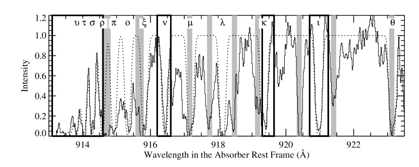
Figure 3: Histogram-style line: Combined FUSE night-time observations of intensities at wavelengths just below the Lyman limit for the absorption system at $z=0.080923$ in front of PHL 1811. In this presentation, the spectrum has been binned to a resolution $\Delta v=6\,{\rm km~{}s}^{-1}$ for easier viewing (best-fit calculations were done at full resolution). Shaded vertical bars indicate positions of easily identified, but irrelevant features, and the boxes enclose regions where the values of $\chi^{2}$ between the observed spectrum and the synthetic trial spectrum (dotted curve) were evaluated. Greek letters indicate wavelength positions of the members of the Lyman series lines.

We found the best solution for the instrumental resolution to be $29\,{\rm km~{}s}^{-1}$ (FWHM for a Gaussian profile), which is on the high side of the range $22-30\,{\rm km~{}s}^{-1}$ found by other FUSE investigators (Heckman et al. 2001; Hébrard et al. 2002; Lebouteiller et al. 2004; Sembach et al. 2004; Williger et al. 2004). A slight reduction in our resolution may have arisen from the difficulty in registering the offsets of individual low S/N observing sessions with respect to each other.

We can use the $\lambda 1302$ O I absorption observed by STIS to indicate the contribution by turbulent broadening. Figure 4 shows the conversion of this feature into apparent optical depths $\tau_{\rm a}(v)$. Here, we can see that the lower portion of the velocity profile approximates a Gaussian distribution with $b=13.2\pm 1.4\,{\rm km~{}s}^{-1}$, which may be reduced to $12.6\,{\rm km~{}s}^{-1}$ when a compensation is made for instrumental smearing. The behavior of the upper portion of the O I profile has no effect on our temperature derivation because the overall strength of the O I feature is much greater than those of the H I Lyman series absorptions that defined $b_{\rm H~{}I}$. (In effect, this portion of the profile should be completely saturated in the H I lines we analyzed.) If we solve the equations

$$b^{2}_{\rm O~{}I}={kT\over 8m_{\rm p}}+b^{2}_{\rm turb}$$ (1a)

$$b^{2}_{\rm H~{}I}={2kT\over m_{\rm p}}+b^{2}_{\rm turb}$$ (1b)

we find that

$$T={8m_{\rm p}(b^{2}_{\rm H~{}I}-b^{2}_{\rm O~{}I})\over 15k}=7070^{+3860}_{-4680}\,{\rm K}$$ (2)

for the preferred values of $b_{\rm H~{}I}$ and $b_{\rm O~{}I}$, with the error limits defined from their worst extremes working in opposite directions.

Figure 4: The apparent optical depth $\tau_{\rm a}(v)\equiv\ln[I_{\rm cont.}/I(v)]$ as a function of velocity for the $\lambda 1302$ feature of O I in the Lyman limit system at $z=0.080923$ in front of PHL 1811. The histogram-style plot shows the observations and their errors. The smooth profile is the best-fit Gaussian function that defines the velocity dispersion of O I, exclusive of the central portion that is indicated with a thin line.

In principle, it is possible that in this analysis we are being deceived by a small amount of hydrogen that could have a much larger turbulent velocity dispersion. For the ratio of H I to O I in this absorption system, Lyman series lines near Ly$\sigma$ (at 914.3 Å), which probably have the most influence in determining $b$(H I), have optical depths about 10 times that of the O I $\lambda 1302$ feature. In essence, our analysis rests on the assumption that the Gaussian profile shown in Fig. 4 remains the same down to $\tau_{\rm a}\sim 0.1$, which may not be true. However, it is reassuring that the observed Ly$\iota$ profile is not wider than the theoretical one, and the fit to the right-hand edge of Ly$\alpha$ shown in Fig. 2 gives a value $b=16.4\,{\rm km~{}s}^{-1}$ with a formal uncertainty in the fit of $0.4\,{\rm km~{}s}^{-1}$. This line is 340 times as strong as Ly$\iota$, which gives us some reassurance that the broadening is indeed purely thermal. Thus, except for hydrogen at negative velocities (shown by the shaded portion of the profile in Fig. 2), the Gaussian shape seems to continue to much lower $\tau_{\rm a}$ levels in the hydrogen lines than we can see in the faintest wings of the equivalent profile in O I.

5 Interpretation of the Spectra

5.1 Electron Density

From our upper limit for $N$(C II^∗), we can derive a limit for the excitation rate of this upper fine-structure level and, in turn, the electron density in the C II-bearing material (which is probably mostly ionized, so we can ignore collisional excitation by hydrogen atoms). The electron density is given by the relation

$$n(e)=0.189T^{0.5}\left[{N({\rm C~{}II^{*}})\over N({\rm C~{}II})}\right]$$ (3)

Since we have only a lower limit for $N$(C II), and one which is probably well below the real value, we can instead use $N({\rm Si~{}II})({\rm C/Si})_{\odot}$ (or the same with S II, since $[{\rm S~{}II/Si~{}II}]\sim 0$) as a proxy for $N$(C II). Numerically, we find that for the temperature and limits thereof expressed in Eq. 2 that Eq. 3 yields the values

$$n(e) \leq 0.032\,{\rm cm}^{-3}~{}{\rm for}~{}T=2390\,{\rm K}$$ (4)

$$\leq 0.056\,{\rm cm}^{-3}~{}{\rm for}~{}T=7070\,{\rm K}$$

$$\leq 0.069\,{\rm cm}^{-3}~{}{\rm for}~{}T=10930\,{\rm K}~{}.$$

5.2 General Patterns of Element Abundances

Table 3: Relative Abundances of Specific Atoms and Ions

Ratio	Value
Species relative to H I
[C II/H I]	$\gg 0.33$
[N I/H I]	$-1.47^{+0.30}_{-\infty}$
[O I/H I]	$-0.17\pm 0.07$
[Si II/H I]	$0.46^{+0.07}_{-0.06}$
[S II/H I]	$0.52^{+0.17}_{-0.25}$
[Ar I/H I]	$<0.44$
[Fe II/H I]	$0.15^{+0.15}_{-0.13}$
Species relative to Si II
[C II/Si II]	$\gg-0.13$
[N II/Si II]	$-0.45^{+0.49}_{-0.41}$
[S II/Si II]	$0.06^{+0.16}_{-0.25}$
[Fe II/Si II]	$-0.31^{+0.14}_{-0.13}$

The top portion of Table 3 summarizes the abundances of various elements with respect to H I, compared to their respective solar abundance ratios. There are striking differences from one element to the next. At the most superficial level, we note that the singly ionized forms of C, Si, S and Fe appear to have supersolar abundances, while those of the neutral atoms N and O are subsolar. The ions all have ionization potentials more than a few eV higher than that of H, while the neutral atoms N and O do not. Thus, the pattern we note here is probably caused by conditions that favor having a substantial amount of the hydrogen in a fully or partially ionized condition, and the hydrogen ions far outnumber the neutral atoms that coexist with the N I and O I.

In the region containing H I, there is a spectacular deficiency of nitrogen with respect to oxygen: [N I/O I] $\lesssim-1.3$. We illustrate the strength of this abundance disparity for these two neutral atoms in Figure 5, where the observed spectrum covering the 1200 Å triplet of N I has three replicas of the 1302 Å feature overplotted on it, each with an apparent optical depth that is rescaled to agree with what the respective underlying N I line would look like if [N I/O I] were equal to zero. Later, in §§5.3–5.5, we will examine the secureness of our conclusion that a low value of [N I/O I] indicates a true underabundance of nitrogen and that it is not simply a consequence of drastically different responses to various ionizing processes.

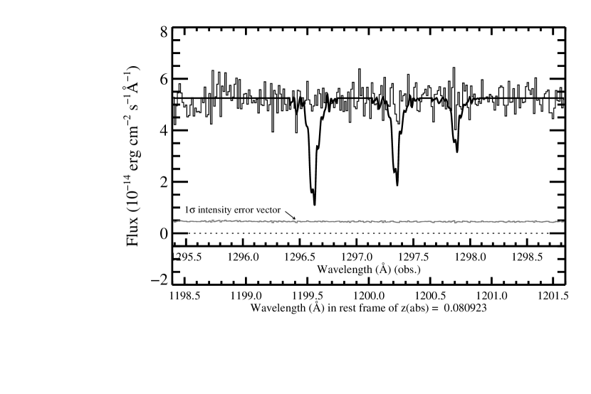
Figure 5: The STIS E140M spectrum of PHL 1811 covering the expected wavelength of the 1200 Å triplet for the Lyman limit absorption system at $z=0.080923$ (Histogram style trace). Overplotted are three replications of the 1302 Å O I feature, but with their optical depths rescaled to show how N I features would appear if N I and O I had the same velocity profiles and relative abundances that agreed with the solar ratio.

To examine the abundance patterns of the ions, we use Si II as a standard, since its abundance has the smallest errors. The bottom portion of Table 3 indicates that Fe and N appear to be underabundant, while the other two elements, C and S, have abundances that are consistent with the solar ratios. The mild underabundance of Fe may be caused by either its depletion onto dust grains, since Fe generally depletes more rapidly than the other elements (Savage & Sembach 1996; Jenkins 2004), or by a smaller contribution from Type Ia supernovae compared to the mix of sources that contributed to the chemical enrichment of our Galaxy.

It is important to note that the atoms within the region are shielded from a uniform, external ionizing radiation field by a column of neutral hydrogen that approaches only $5\times 10^{17}{\rm cm}^{-2}$. Moreover, if the region is porous, or is in a thin sheet inclined to the line of sight, or contains internal sources of ionization (i.e., recently formed stars), the shielding could be considerably smaller. Hence, we cannot simply assume that virtually all atoms or ions in a region containing H I must be concentrated within the lowest stage that has an ionization potential greater than that of hydrogen. It is therefore clear that meaningful interpretations of element abundances must allow for alterations that might arise from elements being distributed in different ionization levels, many of which are unseen. In the three subsections that follow, we consider the consequences of this problem. We start with the possibility that collisional ionization could play a role, and then we examine the effects of photoionization from several different perspectives.

5.3 Collisional Ionization

For the temperature range of the H I-bearing material that we derived in §4.2, there should be negligible ionization of atoms and first ions to higher stages of ionization if the gas is in equilibrium (Sutherland & Dopita 1993). While this may seem to rule out collisional ionization as an important factor, we must not overlook the possibility that the gas might have been very hot at some earlier time and has cooled radiatively. The time scale for such cooling is shorter than the recombination time, so the higher ionization from an earlier time may effectively be “frozen in” at the current epoch, or at least partially so. For a minimum electron density $n(e)=10^{-3}{\rm cm}^{-3}$ that we derive in §5.4 below and a representative rate of recombination for singly-ionized atoms $\alpha(T)=10^{-12}{\rm cm}^{3}{\rm s}^{-1}$ at $T\sim 10^{4}\,$K, the recombination time scale is short: $\tau=[(n(e)\alpha({\rm H},T)]^{-1}=3\times 10^{7}{\rm yr}$. It seems implausible that we are viewing the gas at just the right moment within the probable total lifetime of the system.

5.4 Photoionization in a Uniform Slab Illuminated by the Intergalactic Field

5.4.1 General Considerations

A simple picture to consider is a uniform, infinite slab that is immersed in a bath of ionizing radiation. In this regime, we can implement the CLOUDY ionization code (v94.0, Ferland et al. 1998) and compare the calculations with our observations. We employ CLOUDY following the procedures described in Tripp et al. (2003); we assume that the gas is photoionized by the UV background from QSOs according to the calculations of Haardt & Madau (1996), and we set the intensity of the flux at 1 Rydberg to $J_{\nu}=1\times 10^{-23}$ ergs s^-1 cm^-2 Hz^-1 sr^-1, a value in accord with current observational constraints (Shull et al. 1999; Davé & Tripp 2001; Weymann et al. 2001).

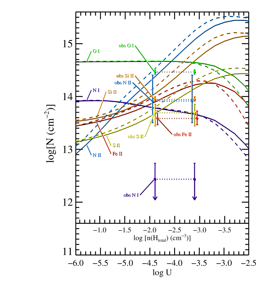
Figure 6: The trends for the logarithms of predicted column densities from a CLOUDY model calculation for different atoms and ions, each depicted by a different color, as a function of the logarithm of the ionization parameter $U$, as seen through a slab perpendicular to the line of sight with a thickness that matches the observed $N({\rm H~{}I})=10^{17.98}{\rm cm}^{-2}$ (solid curves) and irradiated on both sides by an intergalactic radiation field specified by Haardt & Madau (1996). All curves are based on solar abundance ratios of the various elements with respect to hydrogen. The dashed curves show the same information, except that here the slab is assumed to be inclined to the line of sight by $60\arcdeg$, making the physical thickness of the slab smaller by a factor of 2, but with perceived column densities that are increased by the same factor to compensate. An extra scale for the $x$ axis shows the values of $\log n(H_{\rm total})$ (i.e., the sum of the ionized and neutral hydrogen local densities). The pairs of points with error bars show the observed column densities for comparison, located at assigned values of $\log U=-4.4$ and $-3.6$ that seem to give a good agreement with the curves using different criteria (§§5.4.2 and 5.4.3).

Figure 6 shows how the expected column densities of different species vary as a function of the ionization parameter $U$, which equals the ratio of density of hydrogen ionizing photons to the total density of hydrogen (in both neutral and ionized forms). To make the comparisons of the observations and theory easy to interpret in terms of the solar abundances, the intrinsic abundances of the elements in the CLOUDY calculation are set to be equal to the solar abundances. The solid curves depict the outcome for a slab perpendicular to the line of sight, so that the observed column density $N({\rm H~{}I})=10^{17.98}{\rm cm}^{-2}$ equals its true thickness. Of course, there is a good chance that the slab is not perpendicular to our viewing direction. In fact, with random possible orientations the median inclination would be $60\arcdeg$, and under this circumstance the true thickness of the disk (and hence the shielding of material well inside the slab) would be reduced by a factor of 2. The effects arising from this inclination are small, and they are shown by the dashed lines in the figure. The range of temperatures calculated by CLOUDY start from 940 K at $\log U=-6.0$ and increase steadily to 8300 K at $\log U=-2.5$.

The results of our observations of singly-ionized or neutral species in the Lyman limit system are shown in Fig. 6 by the vertical locations of pairs of points with error bars (joined by dashed lines). Figure 1 indicates that the multiply ionized atoms C IV, Si IV and S III (shown in the lowest three panels in the figure) are slightly offset in velocity from the others. Hence, either they arise from a location that is distinctly different from places where the lower excitation species are found, or perhaps they reside in a special boundary region where there is some velocity shear with respect to the region with lower excitation. For this reason, we feel that it is probably unwise to use these stages as a guide for determining the conditions that affect the lower ions. Indeed, we find that the CLOUDY models cannot simultaneously match the column densities of the low and high ions at a single ionization parameter. This corroborates our conclusion that the absorber is a multiphase entity.

In the following two subsections, we explore the outcomes for two different values of $\log U$, a free parameter that we can adjust to give the best level of self consistency for the element abundances.

5.4.2 An Initial Choice for the Ionization Parameter

Table 4: Relative Element Abundances from the CLOUDY Model

	$\log U=-4.4$			$\log U=-3.6$
	at the Indicated Inclinations			at the Indicated Inclinations
Ratio	$0\arcdeg$	$60\arcdeg$		$0\arcdeg$	$60\arcdeg$	Error
[C/H]	$\gg-0.16$	$\gg-0.32$		$\gg-0.75$	$\gg-0.93$	$\cdots$
[N/H]${}_{\rm N~{}II}$	$-0.41$	$-0.56$		$-1.11$	$-1.27$	+0.49, $-0.41$
[N/H]${}_{\rm N~{}I}$	$-1.35$	$-1.35$		$-1.24$	$-1.24$	+0.30, $-\infty$
[O/H]	$-0.20$	$-0.20$		$-0.18$	$-0.18$	$\pm 0.07$
[Si/H]	$-0.11$	$-0.22$		$-0.77$	$-0.88$	+0.07, $-0.06$
[S/H]	0.01	$-0.10$		$-0.47$	$-0.60$	+0.17, $-0.25$
[Fe/H]	$-0.34$	$-0.42$		$-0.66$	$-0.72$	+0.15, $-0.13$

Since the nucleosynthetic origins of O, Si and S are very similar (Wheeler, Sneden, & Truran 1989; Thuan, Izotov, & Lipovetsky 1995; Chen et al. 2002) and the depletions of these elements onto grains is not appreciable in regions of low density (Savage & Sembach 1996; Jenkins 2004), we may start with a provisional assumption that there are not any serious deviations from the solar abundance ratios between these three elements. If we do so, we find that a CLOUDY model with $\log U\approx-4.4$ gives a generally acceptable fit to the observations for most of the low ions, but with a glaring exception for N I. From the flatness of the predictions for O I and the tight error limits associated with our observation of $N({\rm O~{}I})$, together with the knowledge that O usually is only mildly depleted in the ISM of our Galaxy (Cartledge et al. 2001, 2004; André et al. 2003), we may state that the most secure measure of an overall metallicity is given by $[{\rm O/H}]=-0.20\pm 0.07$, which represents the distance the measurement is below the model prediction for a solar abundance ratio. The abundances of other elements depend more sensitively on the assumed value for $\log U$. The left-hand portion of Table 4 shows the element abundances for $\log U=-4.4$; considering that O is slightly subsolar, Si and S seem to have close to their expected abundances, but Fe appears to be depleted by approximately $-0.2\,$dex. The temperature calculated by CLOUDY at this value of $\log U$ is 5900 K, a value consistent with our analysis discussed in §4.2.

5.4.3 Alternative Choice for the Ionization Parameter

While our choice of setting $\log U$ to $-4.4$ gives relative abundances of O, Si, S and Fe that are generally consistent with abundance ratios for stars and the ISM of our Galaxy and other systems, the model indicates a very strong deficiency of N. Beyond this, however, we find an untidy mismatch between the observations and predictions for nitrogen in the neutral and singly-ionized forms. We can obtain a better concordance for these two forms by raising the value of $\log U$, but this comes at the expense of making other $\alpha$-process elements discordant with their solar abundance ratios. If we raise $\log U$ by 0.8 dex to the value $-3.6$, the two values for the nitrogen abundance match each other. The right-hand part of Table 4 shows the abundance ratios of all elements with this higher value of $\log U$. The disparity in the results for the two forms of N vanishes, but N is still very deficient relative to the other elements. It now becomes harder to define an overall metallicity, since the outcome depends on which element one choses as the standard. The predicted temperature of the gas $T=7000\,$K at this new value of $\log U$ is slightly higher than before, but it is still completely consistent with what we derived in §4.2.

We believe that it is unlikely that $\log U$ could be much higher than about $-3.5$ because the disparity between the inferred abundances of different $\alpha$-process elements becomes unacceptably large. If the intergalactic field is the only radiation field present, this finding sets a lower limit on the electron density $n(e)>10^{-3}{\rm cm}^{-3}$. Any local sources of additional ionizing photons, a possibility that we will consider in the following subsection, should raise this limit.

For either choice of the inclination angle and $\log U<-3.5$, nearly all of the silicon is singly ionized. If we accept our finding that $-0.11<[{\rm Si/H}]<-0.88$, depending on our choice for the inclination and $\log U$, our measured $\log N({\rm Si~{}II})=13.95$ implies that the amount of hydrogen in neutral and ionized forms amounts to $18.55<\log N({\rm H}_{\rm total})<19.34$. If the silicon in the system is depleted onto grains (at most, by no more than 0.4 dex – see §5.5), this hydrogen column density could be somewhat larger.

5.5 More Detailed Photoionization Modeling for N and O

The striking difference between the abundances of N I and O I warrants further study. Up to now, we have ignored the possibility that the photoionization of the gas might be enhanced over that provided by the extragalactic radiation field. In this case, one could imagine that we are being misled by the effects arising from an intense, internal radiation field provided by embedded hot stars. The configuration could be such that there would be insignificant shielding of the gas, or much of it, by any layers of neutral hydrogen or helium.

At first glance, we might suppose that any additional ionizing flux should be very weak, since there is empirical evidence that the rate of star formation per unit area generally scales in proportion to the mass surface density to the 1.4 power (Kennicutt 1998). In our Lyman limit system, our estimate for the surface density $N({\rm H}_{\rm total})=10^{18.54}-10^{19.34}{\rm cm}^{-2}=0.04-0.23\,{\rm M}_{\odot}~{}{\rm pc}^{-2}$ derived from $N$(Si II) is considerably lower, for instance, than the indications from H I in the local region of our Galaxy, $N({\rm H~{}I})=10^{20.8}{\rm cm}^{-2}=6.4\,{\rm M}_{\odot}~{}{\rm pc}^{-2}$ (Dickey & Lockman 1990) (and might be lower still if the Lyman limit system is flat and inclined to the line of sight). Nevertheless, we cannot exclude the possibility that we are viewing through a small gap in a disk system that is, in general, considerably thicker than our observations indicate. If this system subtends a small angle in the sky, we probably would not be able to see its starlight because we are blinded by the light from the background quasar.

For this new picture with internal sources of ionization, it might seem that we are confronted with a hopeless task of grasping the enormous range of possible conditions that govern the relative ionizations of various elements and converging upon a limited solution space. However, the problem becomes tractable when we focus on the ratios of species that are only mildly susceptible to the strength of the ionization, and then use other combinations of observed species that are very sensitive to ionization effects to serve as indicators of the general severity of ionizing field. We will use this approach in the analysis that follows.

Our goal is now to try to explain the result shown in Table 3 that [N I/H I] is less than [O I/H I] by about 1.3 dex or more. Fortunately, under most circumstances the neutral fractions of these three elements are coupled to each other by strong charge exchange reactions (Field & Steigman 1971; Steigman, Werner, & Geldon 1971). However, at some point when the ionizing field becomes very strong and/or the densities are low, the coupling will start to break down. We can see this effect for the predictions shown in Fig. 6. The column densities of N I and O I for a fixed value of $N$(H I) are stable for $\log U<-5.0$, but above this value $N$(N I) starts on a slow downward drift. The behavior of $N$(O I) remains flat up to $\log U=-3.5$, beyond which there is a steep decline.

There is good astrophysical evidence to support the notion that ionization effects can lower [N I/O I]. In the local interstellar medium within about 100 pc of the Sun, $[{\rm N~{}I/O~{}I}]\approx-0.2$ instead of the expected value of zero, and this is consistent with the calculated effects of photoionization in a low density medium illuminated by local sources of EUV radiation (Jenkins et al. 2000a; Lehner et al. 2003). It is important to establish whether or not the low value of [N I/O I] in the Lyman limit system under investigation here is a reflection of a true abundance anomaly or, alternatively, simply a consequence an even more severe shift in ionization caused by a strong EUV radiation bath (or that it arises from a combination of the two).

In the Appendix of this paper, we develop the equations that govern the ionization equilibria of H, He and a trace element (either N or O in this study). Using these equations (Eqs. A3a to A8), we have determined the expected ratios for the neutral fraction of N to that of O, $f_{0}({\rm N},T)/f_{0}({\rm O},T)$, in the presence of unshielded radiation fields that are identical to the fluxes computed by Sternberg, Hoffmann & Pauldrach (2003) for 3 different stellar temperatures $T_{*}$ and surface gravities $g$, ones that correspond to spectral types O9.5 I, O7.5 I and O5 I (Vacca, Garmany, & Shull 1996). Our ionization calculations were performed for 3 values of the gas kinetic temperature $T$, equal to the lower limit, best value and upper limit derived in §4.2. For all cases, we evaluated the results for progressively stronger overall intensities (or lower densities). In order to use this information, however, we must define a practical limit for the ratio of the radiation density divided by the particle density.

It is clear from the simple application of the CLOUDY calculation shown in Fig. 6 that the expected amount of Si II responds rapidly to changes in $U$. We can make good use of this behavior, since we have high quality observations of this element for two stages of ionization, Si II and Si IV. (Unfortunately, the Si III $\lambda 1206$ line of the Lyman limit system partly overlaps the Galactic Si II $\lambda 1304$ line.) Thus, to gauge the strength of the ionization we supplemented our calculations for N and O with evaluations of the expected behavior of Si⁺ from the same equations (but with ionization levels one higher than those indicated by Eqs. A3a$-$A5).

Figure 7 shows how $\log f_{0}({\rm N},T)-\log f_{0}({\rm O},T)$ behaves as a function of our ionization strength indicator, $\log f_{0}({\rm Si^{+}},T)-\log f_{0}({\rm H},T)$. At the point where the curves bend sharply downward in the first two figure panels ($a$ and $b$, for $T_{*}=32,000$ and 37,000 K, respectively), the value of Si⁺/H is no longer useful as an ionization index, but somewhat beyond this point Si⁺³/Si⁺ emerges as an indicator. This is important, because at extremely large ratios of radiation density to gas density, Si⁺/H starts to return downward (as shown by the doubling back of the curves in the middle panel $b$). However, we can exclude these extreme values because they would produce higher values of Si⁺³/Si⁺ than the observed ratio of $N$(Si IV) (plus a $1\sigma$ error) to $N$(Si II) (minus a $1\sigma$ error) that should not exceed 0.70. The dashed portions of the curves indicate the regions where this violation occurs. For the highest stellar temperature shown in the right-hand panel $c$, the Si⁺³/Si⁺ constraint is not useful, since the curves double back toward the same general values of $\log f_{0}({\rm N},T)-\log f_{0}({\rm O},T)$.

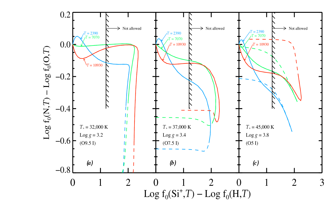
Figure 7: Logarithmic presentations of the expected neutral fraction of N divided by that of O, as a function of the fraction of Si in the singly ionized state divided by the neutral fraction of H. The gas is assumed to be exposed to ionizing radiation fields characterized by the fluxes from supergiant stars at 3 different temperatures $T_{*}$ (Sternberg, Hoffmann, & Pauldrach 2003), as indicated by the label in each panel. Self shielding of the gas by neutral hydrogen or helium is assumed to be negligible. As the curves progress away from the origin, the density of the ionizing radiation divided by that of the atoms increases. The three curves in each panel trace the relationships for the preferred value of temperature derived in §4.2 (green curve) plus reasonable deviations on either side of this temperature defined by the error limits (blue and red curves). Values of $\log[f_{0}({\rm Si^{+}},T)/f_{0}({\rm H},T)]$ to the right of the vertical feathered line are not allowed (see text). The dashed extensions of the curves represent portions of the curves where the predicted value of ${\rm Si^{+3}/Si^{+}}$ exceeds 0.7, which represents our largest value of $N$(Si IV) divided by our smallest $N$(Si II).

We must now use our observations to provide an estimate for the maximum permissible value for $f_{0}({\rm Si^{+}},T)/f_{0}({\rm H},T)$ in our gas system. From Table 3 we reported that $[{\rm Si~{}II/H~{}I}]=0.46^{+0.07}_{-0.06}$. Were it not for ionization effects, we would conclude from our result $[{\rm S~{}II/Si~{}II}]=0.06^{+0.16}_{-0.25}$ that Si is not more depleted than S by more than about 0.22 dex. If we allow for the possibility that S might be slightly depleted and that there are small differences in the response of S and Si to ionization effects (as indicated in Fig. 6), we can adopt a conservative position that the depletion of Si onto grains could be as high as 0.4 dex. If this is true, and we assume that [Si/O] is not appreciably different from zero, we can state that ionization conditions that would be expected to create values of $\log f_{0}({\rm Si^{+}})-\log f_{0}({\rm H})>1.20$ should be excluded by our observations. This limitation is shown by the vertical feathered line in each panel of Fig. 7. Ultimately, we find that to the left of this line $\log f_{0}({\rm N},T)-\log f_{0}({\rm O},T)>-0.12$, $-0.22$ and $-0.30$ for $T_{*}=32,000$, 37,000 and 45,000 K, respectively. In turn, this means that under the most extreme conditions ionization effects should not erode the apparent elemental deficiency of N relative to O by more than 0.30 dex.

Our ionization calculations also indicate that for $\log f_{0}({\rm Si^{+}})-\log f_{0}({\rm H})<1.20$, virtually all of the Si is still singly ionized, that is, in the allowed region all of the changes in the ratio of Si II to H I are caused by changes in the ionization of H. This is a useful finding, since it shows that our earlier determination of $N$(H_total) based on $N$(Si II) is still valid.

6 Reduction and Analysis of the ACS Image

6.1 Basic Reduction

To better understand the origin of the Lyman limit absorption system, we dedicated one orbit of our allocated HST time to obtaining an image of the field using the Advanced Camera for Surveys (ACS) instrument. These data were taken with the Wide Field Camera (WFC) on 05 May 2003 and were archived as a dataset with the root name J8D90501. We used the F625W filter, which is the equivalent of the Sloan Digital Sky Survey $r$-band filter (Pavlovsky et al. 2003).

To aid with the removal of cosmic rays and hot pixels, four separate exposures were taken at four pointings using the ACS-WFC-DITHER-BOX pattern and no CR-SPLIT. The spacing between sub-exposures was 0.265 arcsecs, and each was 520 sec long. The four sub-images were shifted and combined using the ‘multidrizzle’ task available in the dither package of the STSDAS and PyRAF software suite. Fluxes can be obtained from the final co-added image by multiplying the recorded ADU sec^-1 pix^-1 by the inverse sensitivity constant (PHOTOFLAM): we used the most current value available at the STScI web site, $1.195\times 10^{-19}$ ergs cm^-2 s^-1 Å^-1 for the WFC data. These fluxes can in turn be converted to magnitudes and referenced to the ST magnitude zero-point of 21.10. Data from the HRC were not used in our analysis, since no bright galaxies were detected.

Part of the image is reproduced in Fig. 8. We choose to show the region of the data that contains the QSO and the two galaxies at $z\simeq 0.08$ (although we label all the galaxies covered in this region that had redshifts measured in Paper I). The most striking result from the image is that the $z\simeq 0.08$ galaxies appear, at first sight, to be lenticular in shape. The galaxies clearly have a bright bulge at their centers, but both show signs of disks with no spiral pattern, indicative of S0 galaxies. This is particularly interesting, since the origin of S0 galaxies is widely debated.

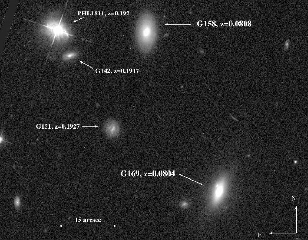
Figure 8: Section of a 2080 s image of the field of PHL 1811 taken with ACS using the F625W filter. Galaxies with redshifts presented in Paper I are identified in the image using the same nomenclature used in that paper. Details about the galaxies G158 and G169 are given in Table 5. An image that covers a much larger field surrounding the quasar is shown in Paper I.

6.2 Surface Photometry

To better quantify the morphology of both G158 and G169, we investigated the surface brightness profiles of the galaxies using the isophote package available with STSDAS [ (Jedrzejewski 1987); see also Milvang-Jensen & Jørgensen (1999) and references therein]. Given a particular value of the semimajor axis $a$ measured from the center of a galaxy, ellipses can be fitted to isophotes of the intensity of light from the galaxy, resulting in a measure of the center of the ellipse, the surface brightness $\mu$ at the value of $a$, the position angle PA of the ellipse, and its ellipticity $\epsilon$. These values can be plotted against $a$, or, more commonly, against the equivalent radius, $r=a\sqrt{1-\epsilon}$. We show the results of ellipse fitting for G158 and G169 in Figure 9, and discuss the results from each in § 7.1 and 7.2.

Figure 9: Results from ellipse fitting to the surface brightness of the two galaxies near $z=0.08$. All quantities are plotted against the equivalent radius, $r=a\sqrt{1-\epsilon}$, where $a$ is the length of the semi-major axis and $\epsilon$ is the ellipticity. Top panel: surface brightness profile, with the best fit of a de Vaucouleurs plus exponential disk fit shown as a solid line. To highlight the disk component, a dotted line shows a fit using only a de Vaucouleurs profile to the inner part of the profile. Second panel: ellipticity $\epsilon$ of the isophotes. Third panel: position angle PA of the isophotes; Fourth panel: Fourier coefficient $B_{4}$ of the isophotes.

One method used to quantify the deviations of a perfect elliptical fit to an isophote is to express the deviations as a Fourier sum. The details of this technique are well documented and are not reproduced here [see the above references for further details; for a discussion of the errors inherent in the fitting process, see, e.g., Rauscher (1995) or Busco (1996)]. Of particular interest is the $B_{4}$ coefficient (the $\cos 4\theta$ term in the Fourier expansion): when $B_{4}>0$, the isophotes are pointed, or ’disky’, whereas when $B_{4}<0$ the light is distributed in a more rectangular shape. Thus $B_{4}$ can serve as a useful discriminator of galaxy type: although $B_{4}=0$ for regular elliptical galaxies, and $B_{4}<0$ for more boxy ellipticals, $B_{4}>0$ can indicate the presence of an S0 galaxy. We examine the values of $B_{4}$ for both G158 and G169 below.

A second way to examine the nature of the galaxies is to measure the disk and bulge components seen in the surface brightness profiles. To that end, we fitted theoretical profiles to the observed values of $\mu$ by minimizing the value of $\chi^{2}$ between the fit and the data. We adopted the simplest profile: a de Vaucouleurs $r^{1/4}$ profile for the bulge component added to an exponential profile for the disk component. When the intensity profile of a galaxy is converted to surface brightness, these profiles become:

$$\mu = \mu_{e}+8.325[(\frac{r}{r_{e}})^{1/4}-1]$$ (5)

$$\mu = \mu_{0}+1.086\>\frac{r}{r_{d}}$$ (6)

where $r_{e}$ and $r_{d}$ are the scale lengths of the bulge and disk components respectively, and $\mu_{e}$ and $\mu_{0}$ are the surface brightness values at those radii.

Our profile fits to the surface brightness profiles of G158 and G169 are shown in the top panels of Fig. 9 and discussed in §§ 7.1 and 7.2. We only fitted points beyond twice the FHWM of the core of the ACS Point Spread Function, or $\approx 0.18$ arcsec (a distance that corresponds to 3.6 ACS WFC pixels, since each pixel is 0.05″ pix^-1). At smaller radii, the surface brightness turns over due to the finite resolution. We note that other, more complicated bulge profiles could have been used for the fit. However, the simple $r^{1/4}$ profile is sufficient for our purposes of identifying the bulge component in our galaxies.

The conversion to magnitudes also included three corrections. We first subtracted 0.13 mags to account for Galactic extinction: we assumed $A_{r}=2.5\>E(B-V)$ (Fitzpatrick 1999) and calculated $E(B-V)=0.05$ from the dust maps of Schlegel et al. (1998). Second, we subtracted a $k$-correction of $2.5\log(1+z)=0.08$ mags. This term was expected to be small for all galaxy types at such a low redshift (Fukugita, Shimasaku, & Ichikawa 1995). Finally, we subtracted a value of $10\log(1+z)=0.34$ mags to account for cosmological dimming of the surface brightness. No correction was made for extinction internal to the galaxies, since we have no information on the magnitude or type of the extinction.

The parameters deduced from the surface brightness profiles are given in Table 5. From these values, we can derive the disk-to-bulge ($D/B$) ratio. If $I_{e}$ and $I_{d}$ are the intensities corresponding to $\mu_{e}$ and $\mu_{0}$, then the bulge fraction ($B/T$) is given in the usual way by

$$B/T=\frac{r_{e}^{2}I_{e}}{r_{e}^{2}I_{e}+0.28r_{d}^{2}I_{d}}$$ (7)

with $D/B$ = ($T/B$)$-$1 (Binney & Merrifield 1998). The values of $D/B$ are given in column 8 of Table 5 and are used in §§ 7.1 and 7.2 to further indicate the morphological types of G158 and G169.

Also included in Table 5 are the measured and absolute magnitudes of the galaxies, $m_{r}$ and $M_{r}$, respectively. Apparent magnitudes were initially measured using sextractor (Bertin & Arnouts 1996); the values were compared with the integrated counts available from the ellipse fitting routine, and found to be identical with the sextractor values when integrated to the last reliable isophote. The absolute magnitudes were derived from $m_{r}$ after correcting for Galactic extinction and applying the $k$-correction given above.

6.3 Unsharp Masking

Finally, we have used the technique of unsharp masking (Malin, Quinn, & Graham 1983) to highlight some of the small-scale structure in G158 and G169. Unsharp masking suppresses large-scale, low-frequency variations, and emphasizes small-scale brightness variations. Example of how useful this technique can be for galaxies observed with HST can be found in, e.g., Erwin & Sparke (2003). To produce our unsharp masks, we smoothed the original data by convolving it with a Gaussian function of width $\sigma=5$ pixels, then subtracted this from the original image. To produce a ’final’ image, the unsharp mask can be added back to the original data. The results for G158 and G169 are shown in Fig. 10. For each galaxy, we show the original image (top panel), the unsharp mask (middle panel), and the ’final’ image (bottom panel). Our interpretations of the unsharp masks for the galaxies are given later in §7.1 and §7.2.

Table 5: Properties of galaxies close to the PHL 1811 sight line at $z=0.08$

					Surface Brightness Parameters
Designations			$\rho$			$r_{e}$		$r_{d}$
Paper I	2MASS	$z$	($h^{-1}_{70}\,$ kpc)		$\mu_{e}$	(′′)	$\mu_{0}$	(′′)	$D/B$		$m_{r}$	$m_{J}$	$m_{H}$	$m_{K_{s}}$	$M_{r}-5\log h_{70}$
(1)	(2)	(3)	(4)		(5)	(6)	(7)	(8)	(9)		(10)	(11)	(12)	(13)	(14)
G158	J21545996$-$0922249	0.0808	34		19.48	0.51	20.24	1.47	1.2		17.48	15.68	14.95	14.63	$-20.5$
G169	J21545870$-$0923061	0.0804	87		19.51	0.73	20.11	1.00	0.3		17.22	15.15	14.38	13.96	$-20.8$

Note. — Column entries:

Col. (1): Galaxy designation, as given in Paper I;

Col. (2): Designation in the 2MASS point-source catalog;

Col. (3): Galaxy redshift, as reported in Paper I;

Col. (4): Separation between QSO and galaxy on the plane of the sky, assuming $q_{0}=0$;

Col. (5): Surface brightness at the effective radius $r_{e}$ as measured in the F625W band, in mag arcsec^-2, for the component of the surface brightness profile fit given by a de Vaucouleurs profile;

Col. (6): Effective radius, in arcsec, of the same de Vaucouleurs profile;

Col. (7): Surface brightness at the disk length $r_{d}$ as measured in the F625W band, in mag arcsec^-2, for the component of the surface brightness profile fit given by an exponential brightness distribution. NB., Both $\mu_{e}$ are $\mu_{0}$ are corrected for Milky Way extinction (0.13 mags), cosmological expansion [10$\log$(1+$z$) = 0.34 mags], and $k$-correction [$2.5\log$(1+$z$)= 0.08 mags];

Col. (8): Disk length, in arcsec, for the same exponential brightness distribution;

Col. (9): Disk-to-bulge ratio from Surface Brightness profile fits—see text;

Col. (10): Total magnitude of galaxy measured through the ACS F625W filter;

Cols. (11$-$13): $J$, $H$ and $K_{s}$ profile-fit magnitudes listed in the 2MASS point-source catalog;

Col. (14): Absolute magnitude of galaxy, from $m_{r}$, after correction for Milky Way extinction and $k$-correction.

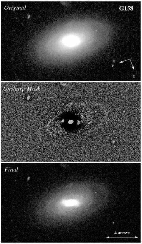
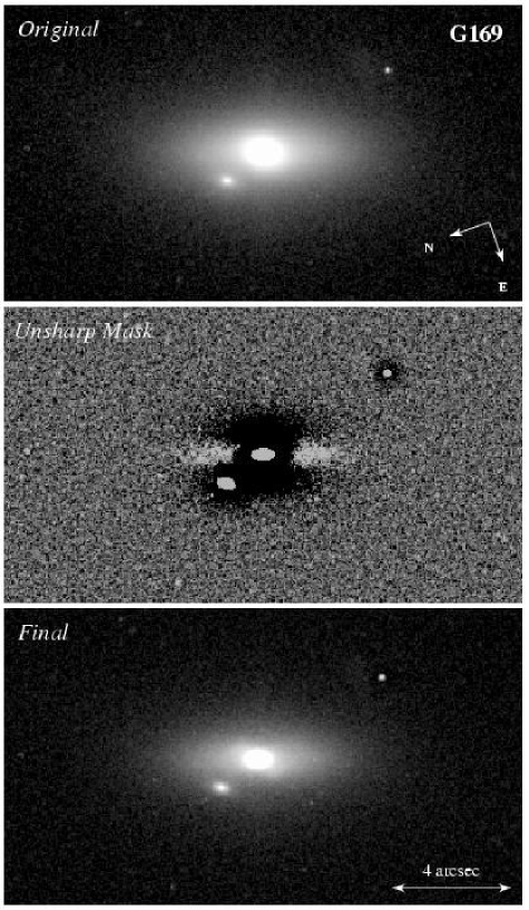
Figure 10: Gray scale representations of G158 and G169 reproduced from the ACS F625W image. Top panels show the galaxies as detected from the final drizzled image, plotted on a logarithmic scale. The middle panels show the unsharp mask of the galaxies, produced by smoothing the original image with a Gaussian of width $\sigma=5$ pixels, then subtracting it from the original. The final image is the sum of the unsharp mask and the original image, plotted with the same logarithmic scaling as used for the top panel.

6.4 PSF Subtraction

A persistent problem when searching for galaxies that might be responsible for quasar absorption lines is that the absorbing galaxy may be so small and well centered along a sightline that it cannot be detected against the glare of the bright background source. To help overcome this problem, one can subtract a properly scaled version of the instrument’s point spread function (PSF) in an attempt to remove the extended pattern of light from the image of the background object. Any believable features detected after the PSF cancellation arise either from the host galaxy of the QSO, or from an object that could, in principle, be at the redshift of the intervening absorption line system.

The high spatial resolution of the ACS offers a powerful tool for searching for objects close to a QSO sight line. One disadvantage, however, is that the PSF is a complicated two-dimensional function whose shape varies with time and field position (for a variety of reasons—see, e.g. Krist (2003)). The use of the ACS coronagraph has proved to be particularly effective in suppressing the central intensity from bright sources (Clampin et al. 2003), including QSOs (Martel et al. 2003). Unfortunately, we had insufficient time available to execute a coronagraphic exposure of PHL 1811 with the suitable PSF control sample. Instead, we made a normal exposure with the intent of using a nearby star in the field to act as a model for the PSF.

The core of PHL 1811 in our image is saturated, with the excess charge bleeding down the columns that were centered on the QSO. The radial structure of the PSF is clearly visible, since the brightness of the QSO ensures that the wings of the PSF are captured with moderate S/N. To provide a PSF with a similar charge saturation, column bleed, and S/N in the wings (in order to provide better subtraction in that region), we elected to use the one star in the field with a brightness similar to that of PHL 1811. To obtain the best possible subtraction, we fitted the stellar PSF to the QSO PSF by minimizing the $\chi^{2}$ statistic, allowing a shift in the stellar PSF image to vary in both the $x$ and $y$ direction, as well as a multiplicative brightness scale factor between QSO and stellar PSF, and a rotation of the PSF about its center (which overcomes the effect of remapping to correct for the field distortion). The results are shown in Fig. 11 and are discussed below in §7.3.

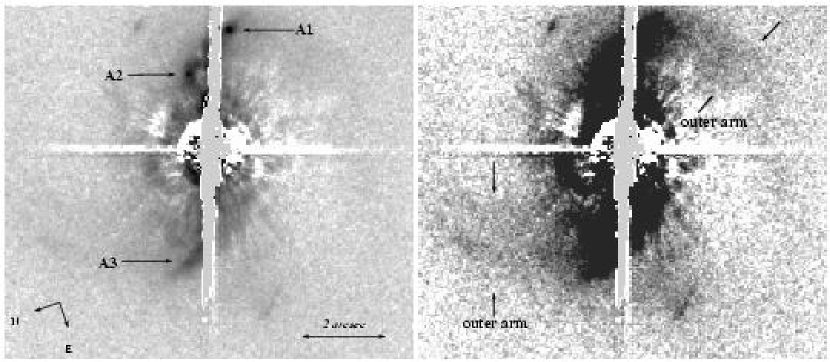
Figure 11: Results of subtracting a PSF of a nearby star from the QSO. Both panels show gray scale representations of the same image, plotted on a logarithmic scale, but the right-hand panel has a more extreme stretch to show the possible presence of outer spiral arms, which are likely to arise from the host galaxy. At the redshift of the QSO, the 2″ bar shown at the bottom of the left-hand panel corresponds to 6.4$h^{-1}_{70}\,$ kpc. The labels A1, A2 and A3 are used to indicate bright nebulous regions in the image that are discussed in the text.

7 Interpretation of the ACS Image

7.1 G158

G158 is the galaxy closest to the PHL 1811 sight line with a redshift that is similar to that of the Lyman limit system. At the redshift $z=0.0808$ reported in Paper I, the separation of $22\farcs 9$ from the line of sight corresponds to a lateral distance of 34 $h^{-1}_{70}\,$ kpc. We measured an $r$-band magnitude of G158 equal to 17.35 using the methods described in §6.1, after correcting for Galactic extinction (§6.2) but with no $k$-correction. We can compare the resulting absolute magnitude $M_{r}-5\log h_{70}=-20.43$ with those of other galaxies at a similar redshift. Blanton et al. (2003) have derived the $r$-band luminosity function for galaxies at $z\simeq 0.1$ in the SDSS. They find that an $L^{*}_{r}$ galaxy at $z=0.1$ has an absolute magnitude of $M^{*}_{r}-5\log h_{70}=-21.21$. Since the difference in the $k$-correction between a galaxy at $z=0.08$ and $z=0.1$ is negligible, G158 is therefore a $0.5L^{*}_{r}$ galaxy.

The left hand panel of Fig. 9 shows the results of our surface photometry analysis of G158. The surface brightness profile shows a clear deviation from the $r^{1/4}$ law beginning at $r\approx 0.9$″. The deviation is easily accounted for by fitting an exponential disk model. The presence of a disk with no obvious spiral arm patterns suggests that the galaxy is of type S0. It is interesting to note, however, that the unsharp mask image presented in the middle panel of Fig. 10 reveals faint rings in the galactic disk, which may be residuals of spiral arm structures, which were once more prevalent in the ealier history of the galaxy. However, since these features would not normally be apparent in unprocessed images, it seems appropriate to retain the classification of G158 as an S0 galaxy. The disky nature of the galaxy is also suggested by the peak in a positive value of $B_{4}$ at a similar radius. The $D/B$ ratio is 1.2, which lies in the middle of the range expected for S0 galaxies, $0.1<D/B<2$ (Burstein 1979; Kent 1985; Bothun & Gregg 1990).

Also intriguing is the peak in the PA. Such maxima, combined with peaks in ellipticity, are often associated with a galactic bar. We see little evidence in our data for a well defined maximum in $\epsilon$ to accompany the peak in PA, but there are examples in nearby galaxies where a bar (or some other feature) does not have an obvious ellipticity peak (Erwin & Sparke 2003). If we look at the unsharp mask in Fig 10, we can see small peaks of emission at the edge of the dark ring that surrounds the nucleus of the galaxy. Since the end of bars in early type galaxies have sharp cutoffs in their luminosity profile (Ohta, Hamabe, & Wakamatsu 1990) galactic bars often show up well in unsharp mask images (which emphasize small-scale, high frequency structures). The features seen in Fig. 10 do not extend all the way to the center of the galaxy, but are suggestive of the existence of a bar. Similar features can be seen arising from the bars in the unsharp masks of NGC 2880, NGC 2962, NGC 6654 presented by Erwin & Sparke (2003). When the unsharp mask image is combined with the original to give the ‘final’ image shown at the bottom of Fig 10, the bar shows up convincingly. For these reasons, we extend our classification of G158 to that of an SB0 galaxy.

7.2 G169

G169 is the other galaxy in the field that we were able to identify at a redshift near that of the Lyman limit system. Again from Paper I we find $z=0.0804$, a separation of $58\farcs 9$ from the line of sight, and an impact parameter of 87 $h^{-1}_{70}\,$ kpc. Our current $r$-band magnitude measurement of G169 is 17.09 when corrected for Galactic extinction (and no $k$-correction), which corresponds to an absolute luminosity of $M^{*}_{r}-5\log h_{70}=-20.69$. Again using the value of $M^{*}_{r}$ from Blanton et al. (2003), we find that G169 is a $0.6L^{*}_{r}$ galaxy, similar to that of G158.

The right-hand panel of Fig. 9 shows the results of our surface photometry analysis of G169. The surface brightness profile is close to that expected for an $r^{1/4}$ law, but there is a small deviation at $r\approx 1$″, which can be accounted for using a disk exponential profile. The $B_{4}$ coefficient also shows positive values at 1″ and beyond. Although the high inclination of the galaxy makes it hard to see any spiral structure which may exist, no spiral features are obviously present. This fact, combined with the detection of a weak disk, again leads us to classify G169 as an S0 galaxy. The $D/B$ ratio of G169, 0.3, is consistent with that of S0 galaxies, which as noted above, have $0.1<D/B<2$.

Both the PA and ellipticity profiles show peaks, again suggesting the presence of a bar. However, the maxima do not coincide at the same radius. The unsharp mask also shows emission at the edges of the dark ring surrounding the core of the galaxy, but we interpret these as being due to the disk of the galaxy. Hence the case for the existence of a bar is much weaker for G169 than for G158.

We also note the presence of a possible companion north of the center of G169, 1.56″ from the center of the galaxy. Although this object could be unassociated with G169 and merely lie fortuitously along the line of sight, it may also be a satellite of G169. Such satellites may not be uncommon: Madore, Freeman & Bothun (2004) find that isolated elliptical galaxies often have $+1.0\pm 0.5$ companions within a projected radius of 70 $h^{-1}_{70}\,$ kpc. We estimate that the satellite has an observed magnitude of $r\simeq 21.3$, which would correspond to $M_{r}=-16.9$ (after correction for Galactic extinction and $k$-correction).

A broad, tail-like structure extending from G169 toward the south is barely visible in the ACS picture, but it is more easily seen in the image taken from the ground that was reported in Paper I. This structure may be indicating that some tidal interaction may have occurred, but the tail does not point toward the direction of our sight line to PHL 1811.

7.3 QSO

The results from removing a stellar PSF from the center of PHL 1811 are shown in Fig. 11. We show the results twice at two different stretches to emphasize different features. The PSF subtraction is far from perfect, which is to be expected primarily because of differences in the structure of the PSF as it varies with position across the WFC field of view, and also because the star has a somewhat different spectral energy distribution than the QSO, as indicated by the photographic magnitudes given in the footnote in §6.4. Some of the radial ’spokes’ which are a common feature of ACS PSFs have been removed successfully, but some remain, and the inner diffraction rings can still be seen.

We do not believe that any feature seen within $\sim 1\farcs 5$ of the quasar should be considered real. However, we identify certain structures farther out which do appear to be genuine. At the top of the left-hand panel of Fig. 11 we identify at least two nebulous cores (which we label A1 and A2) that lie in a meandering ‘snake’ of emission, which winds from the top right quadrant to the top left quadrant and down towards the center of the QSO. We also detect an arc of emission, labeled A3, which appears from under the saturated column in the bottom left quadrant. None of these features are artifacts of the PSF subtraction, since A1 and A3 are just visible in the original image before the PSF was subtracted (see Fig. 8). Nor are they inherent features of the ACS PSF wings, since they are not aligned with the usual radial features or the diffraction rings seen in ACS PSFs; no other stellar PSFs in the field show similar images; and synthetic PSFs generated by the software program TinyTim do not show such features.

The right-hand panel shows the results of our PSF subtraction at a much harder stretch. The features labeled in the left-hand panel are clearly burned out, but the snake in which A1 and A2 are embedded is seen to be much wider. Even more significant is the apparent presence of outer spiral arms. The arm in the lower left quadrant is connected to the arc A3; and while part of the emission in the inner upper right quadrant is lost because of poor PSF subtraction, there is good evidence for a second spiral arm at the outer edge of the quadrant. The emission can be traced out to 3.8 and 4.8″ for the arm in the upper right and lower left quadrants, respectively.

The results from the PSF subtraction therefore appears to indicate the presence of a spiral galaxy directly in front of, or surrounding, the QSO. This could be responsible for the Lyman limit system at $z=0.080$. Alternatively, the object could be the host galaxy of the QSO at $z=0.192$. The detection of a QSO shining through the center of a faint galaxy is not unprecedented: we detected such an alignment of the low surface brightness galaxy SBS 1543+593 in front of the quasar HS 1543+5921 for example (Bowen, Tripp, & Jenkins 2001). Nevertheless, it is still striking from Fig. 11 that the central AGN appears to lie exactly at the center of the disk structure, which suggests that we are seeing the host of the QSO.

8 Large Scale Structure of Galaxies near PHL 1811

To understand the distribution of galaxies close to the sight line of PHL 1811, we searched the third data release (DR3) of the SDSS (Abazajian et al. 2004) within four degrees of the position of PHL 1811 using the SDSS SkyServer. We used the galaxy “view”, which is a subset of the PhotoPrimary imaging catalog containing objects classified as galaxies. This classification is based on identifying resolved objects, and includes no spectrographic information. We selected galaxies with Petrosian magnitudes $r<17.7$, which is the magnitude at which the SDSS aims to be complete spectroscopically (Strauss et al. 2002). The results are shown in the top panel of Fig. 12. The SDSS apparently covers a strip of the sky $\sim 2$° wide, running north of the PHL 1811 sight line, just missing the QSO itself. To collate the available redshift information, we performed the same search using the SpecObj view, which contains a cleaned catalog of available spectroscopic information taken from the SpecObjAll table of the DR3. The galaxies identified spectroscopically are shown in the bottom panel of Fig. 12.

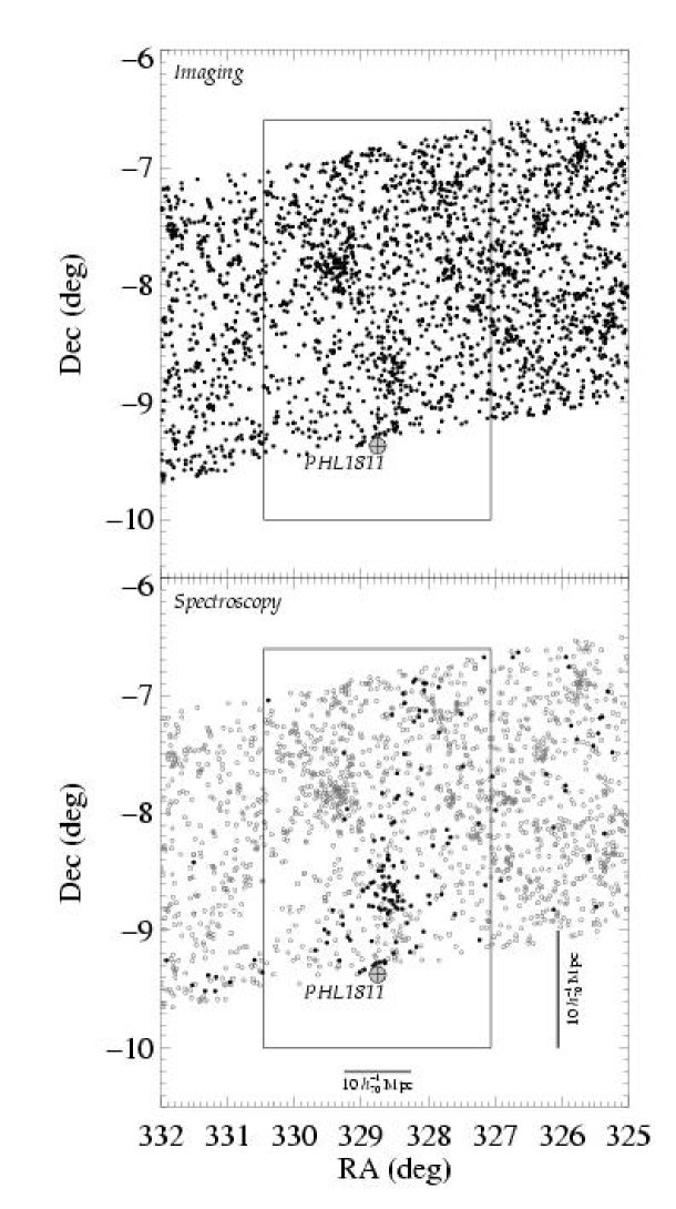
Figure 12: Top panel: the distribution of objects cataloged by DR3 of the SDSS near the sight line of PHL 1811, for objects identified as galaxies on the available CCD data, and with Petrosian $r$-band magnitudes $<17.7$. Bottom panel: positions of objects with $r<17.7$ confirmed spectroscopically as galaxies, and with $z>0.001$. The galaxies indicated with filled circles lie in the interval $0.070<z<0.080$. The overplotted rectangle indicates the survey area used in Fig. 13. The lengths of the bars in the lower panel indicate comoving distances of $10\,h_{70}^{-1}{\rm Mpc}$ at $z=0.08$.

In the bottom panel of Fig. 12 we have highlighted the galaxies found in the redshift interval $0.070<z<0.080$, the interval that covers the Lyman limit system discussed in this paper, as well as the other metal-line absorption systems detected at slightly lower redshifts at $z=0.07344,0.07779$ and 0.07900. The figure shows the galaxies in this redshift range are largely confined to a narrow strip in right ascension (RA) centered at 328.5° and that spans at least 2° in declination (Dec), with a significant conglomeration of galaxies at [RA,Dec] = [328.5,$-$8.7]°. We explore this distribution further in Fig. 13: the top panel shows the redshift distribution of galaxies with Dec, including all galaxies within a 3.4° interval over a range $327.06<$ RA $<330.46$. It is striking that the galaxies appear to follow a line from the top left of the figure to the bottom right, indicative of a filament, or sheet, of galaxies. The cut shows that the two S0 galaxies at $z=0.080$ discussed in §7.1 and §7.2 (not plotted here, since they were not covered by the SDSS) lie at the edge of the filament, assuming that the filament would continue to run to the south of the QSO line of sight (obviously, more data are required to confirm such an assumption).

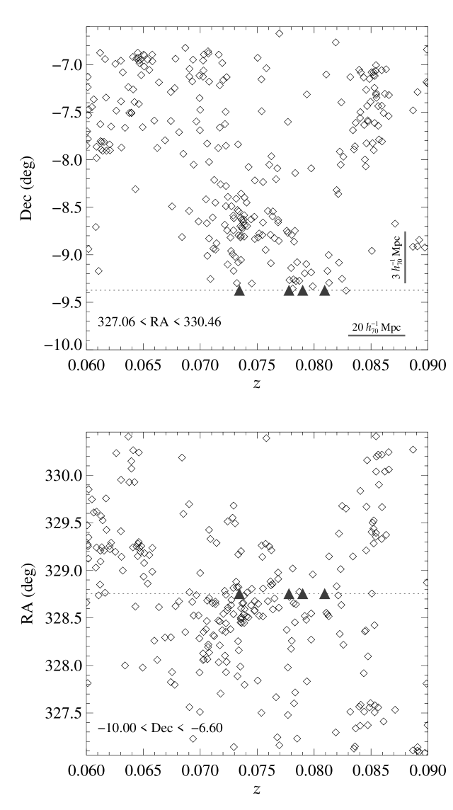
Figure 13: Distribution in redshift of $r<17.7$ SDSS galaxies with: top panel—declination, summed over a 3.4° right ascension interval; bottom panel—right ascension, summed over a 3.4° declination interval. The sight line to PHL 1811 is shown as a dotted line, and the redshifts of the absorption systems are indicated by triangles. The lack of galaxies below Dec $\simeq-9.5$ in the top panel is due to the limited coverage of DR3.

A comparison between the objects cataloged in the galaxy catalog and those in SpecObj over the enclosed area of the sky shown in Fig. 12 suggests that the spectroscopic observations are 72 % complete over the magnitude range $14<r<17.7$, with the fraction of incompleteness roughly the same at all magnitudes over that range. Given this high level level of completeness, and that the redshift interval shown is small, the clustering evident in Fig. 13 is likely to be real, and not a result of incompleteness in the SDSS redshift survey.

The bottom panel of Fig. 13 shows a similar distribution of galaxies with redshift but with a cut made orthogonally to the view in the top panel. In the lower diagram, we sum galaxies over the interval $-10.0<$ Dec $<-6.60$ and plot their RA as a function of $z$. This distribution in RA is less well defined than the cut in Dec, but shows that the galaxies seen at the top left of the upper panel tend to be confined to the upper left of the lower panel. This may suggest that the galaxies are distributed in a more filamentary structure, rather than as a sheet.

Bregman, Dupke & Miller (2004) have noted that the direction toward PHL 1811 is not far from a line in the sky that extends from the clusters Abell 2402 (50′ away at $z=0.0809$) and Abell 2410 (109′; $z=0.0809$) to Abell 2376 (136′; $z=0.0896$) and Abell 2377 (139′; $z=0.0808$), all of which lie within the Aquarius B Supercluster. The fundamental theme of their paper is that lines joining clusters are probably more likely than usual to be near over-dense accumulations of the warm-hot intergalactic medium (WHIM), a conclusion suggested by the outcomes of hydrodynamical simulations of structure formation in the universe (Cen & Ostriker 1999; Davé et al. 2001). The redshifts of these clusters are remarkably close to each other and to that of the Lyman limit system under study here. Unfortunately, the clusters and the line joining them are at a declination just below the southern limit of the SDSS, so we are not able to check whether or not there is an enhancement in the density of galaxies near the line.

9 Discussion

9.1 Chemical Evolution

The relative proportions of different elements in either stars or an interstellar medium convey important information on the history and nature of the nucleosynthetic sources in a particular environment. This is a rich field of study, but one that presents major theoretical challenges to interpret the many factors that can influence the enrichment process, ranging across such topics as the star formation rates and how they vary with time, the distribution of stellar masses (which may also change with time), the inflow of pristine material from outside the system, and the loss of gas into the intergalactic medium, either through SN-driven winds or dynamical processes [see Matteucci (2001) for a coverage of many of the fundamentals these subjects]. In this section, we will explore some implications that arise from our findings on relative element abundances in the Lyman limit system at $z=0.08$ in front of PHL 1811. In turn, this information provides insights on the properties of probable contributors to the gas that we will discuss in §9.2.

We return to our conclusions on the abundance ratios of the elements that arose from the CLOUDY calculations for a slab inclined by $60\arcdeg$ to the line of sight, as presented for two values of $\log U$ in Table 4. These two conditions represent our most plausible choices for the state of the gas that is exposed to the intergalactic radiation field, but without any appreciable influence from possible internal sources of ionization. Both values of $\log U$ have certain ways of deviating from our usual expectations however. For the lower value of the ionization parameter, i.e., $\log U=-4.4$, the $\alpha$-process elements O, Si and S have relative abundances consistent with their solar abundance ratios, while for N we obtain different abundances derived from $N$(N I) and $N$(N II), which may reflect real differences in a poorly mixed system with varying levels of ionization. The opposite is true for the other choice for $\log U$, i.e., the one equal to $-3.6$: the two nitrogen abundances are consistent with a single (low) abundance of N, but there are mild disparities in the abundances of the $\alpha$-process elements compared to their solar values. For either choice of $\log U$, several important facts emerge: (1) the abundance of O is slightly sub-solar, (2) the abundance of N, even if it varies somewhat, is far below that of O, compared to the solar abundance ratio and (3) the value of [Fe/O] is somewhat below zero. As is usually the case when Fe is compared to O or some other $\alpha$-process element, it is not certain if a deficiency of Fe is caused by the formation of dust grains or a relative lack of production by Type Ia supernovae.

For the moment, we focus on the result for nitrogen when $\log U=-4.4$ in the CLOUDY model. In this case, the two forms of N that we observe, neutral and singly-ionized, present an intriguing dilemma since they give mutually inconsistent results for the abundance of this element. This disagreement is not strong, however, since the $+1\sigma$ limit for [N/H] based on N I is only slightly below the $-1\sigma$ limit based on N II. These error limits do not include additional deviations that might arise from uncertain assumptions in the CLOUDY model or atomic parameters. Nevertheless, if we accept at face value the possibility that nitrogen is very deficient with respect to other elements in the H I-bearing material but is closer to normal in the more fully ionized gas, we must adopt the notion that we are viewing a chemically inhomogeneous gas system. One possibility is that the gas complex is not simply an intergalactic cloud, but is a system of gas and stars that has some internal H II regions that have been specially enriched by some bursts of star formation. This is not a new concept; it is one that has been proposed for the blue compact dwarf galaxies Mrk 59, I Zw 36, I Zw 18 and NGC 1705, based on the observed differences of abundances in their H I and H II regions (Thuan, Lecavelier des Etangs, & Izotov 2002; Aloisi et al. 2003; Lebouteiller et al. 2004; Lee & Skillman 2004; Aloisi et al. 2005, in preparation). While we do not see stars or H II regions in our ACS image, it is possible that our ability to do so was compromised by the glare of the quasar (§6.4), or that perhaps the spiral galaxy discussed in §7.3 is indeed the Lyman limit system and not the quasar’s host galaxy. Of course, this dichotomy departs from our simple construct of a chemically homogeneous cloud whose ionization is maintained by an external radiation field, and for the more fully ionized gas we may be approaching a regime that more closely approximates the locally enhanced ionization conditions discussed in §5.5. Even in the light of this more complex picture, we can still maintain that our determination of the range of $N({\rm H}_{\rm total})$ (§5.4) should remain intact because it encompasses our worst extremes for [Si/H], and in all circumstances most of the Si is in the form of Si II.

We now switch to considerations that arise when $\log U=-3.6$. Here, the two forms of N give a consistent result in the simple CLOUDY model, [N/H] = $-1.25$, but while [O/H] still remains at a level near $-0.2$, the abundances of the other two $\alpha$-process elements decrease to lower amounts, ranging from $-0.88$ for [Si/H] to $-0.60$ for [S/H]. As we stated earlier, these elements are generally considered to have a common origin. Even so, there is some evidence from the analyses of stars in the thin disk of our Galaxy that as metal enrichment progresses (as measured by [O/H]), there are gradual increases in [Mg/O] and [Si/O] (Bensby, Feltzing, & Lundström 2004). In essence, the abundances of Si and O do not necessarily increase exactly in lock step with each other (and this may apply to S as well). On the theoretical side, the composition of supernova ejecta in the models of Woosley & Weaver (1995) show that supernovae with initial masses of about 35 M_⊙ have strong yields of O with much less production of Si and S, while the converse is true for progenitor stars in the range $15-25\,{\rm M}_{\odot}$. Thus, our findings may reflect upon a stronger than usual emphasis of high mass stars in the mix of progenitors for the Type II supernovae that created the elements. In turn, we could interpret the excess of O relative to other $\alpha$-process elements to arise from either an initial mass function (IMF) that is skewed more toward higher masses, relative to the IMF of our Galaxy, or by the fact that our sample is dominated by gas that was enriched very soon after a burst of star formation where only the highest mass stars had a chance to evolve to the supernova stage.

Irrespective of the value of $\log U$ (between the two extremes we have chosen), there is a clear deficiency of nitrogen. The study of this element relative to the $\alpha$-process elements in different astrophysical sites is useful because [N/$\alpha$] increases as a system ages and intermediate-mass stars (and stars from later episodes of star formation) have a chance to inject additional nitrogen into the interstellar gas. Deviations in the trend of [N/$\alpha$] versus a general measure of metallicity, such as [$\alpha$/H], can give insights on the star formation history within a gas system or its stellar mass function. For instance, Pilyugin, Thuan & Vílchez (2003) have argued that galaxies that had most of their star formation at an early time have higher N/O trends vs. O/H than those for which most of the stars formed more recently.

However, nitrogen nucleosynthesis is a complicated topic, one that is not yet fully understood. Fundamentally, carbon and oxygen must already be present in the region of the star where fusion occurs in order for nitrogen to be synthesized. Consequently, two nitrogen production channels have been recognized: (1) “primary” nitrogen production, in which carbon and oxygen are first produced in the star and then are mixed into a region where nitrogen is subsequently created from the mixed-in C/O, and (2) “secondary” nitrogen production, in which the star forms from gas that was already enriched with C and O from previous generations of stars. Nitrogen nucleosynthesis trends vs. time depend on various factors, including the initial metallicity of the interstellar gas, the masses of stars that predominantly contribute to the primary and secondary N production, and whether or not stars of various masses rotate. Izotov & Thuan (1999) have suggested that massive stars play an important role in primary nitrogen synthesis. In low-metallicity blue compact galaxies, they argue that the oxygen and nitrogen come from the same massive stars, and there is no delay between the time of the oxygen and (primary) nitrogen enrichment. Stellar rotation can enable massive stars to synthesize primary N, but Meynet & Maeder (2002a, b) conclude that stellar rotation will actually cause intermediate-mass stars to be the main source of primary nitrogen, in which case there should be a lag between the oxygen enrichment and the nitrogen injection. If rotation is not important, then primary N synthesis can occur when C and O from a He-burning core diffuse into a hydrogen-burning shell, the so-called “hot bottom burning;” this should also occur mainly in intermediate-mass stars (Marigo 2001). At any rate, a nitrogen underabundance indicates that a system is young because either the enriching stars are early-generation stars formed in initially low-metallicity gas, or there has not been sufficient time for longer-lived intermediate-mass stars to contribute N to the interstellar gas (or both).

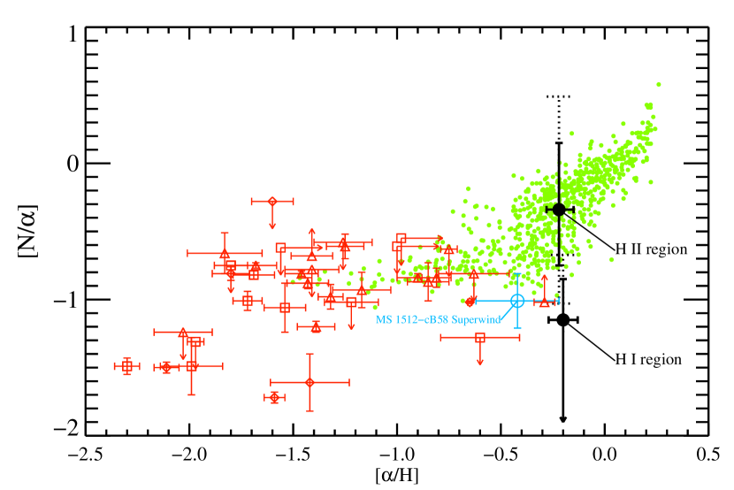
Figure 14: Observed trends in the ratios of nitrogen to $\alpha$-process elements as a function of the ratios of an $\alpha$-process element to hydrogen. Large black dots with error bars: Our determinations for the regions containing mostly ionized gas (upper point) and gas containing some neutral hydrogen (lower point) for the CLOUDY model results for $\log U=-4.4$ listed in Table 4 for a slab of gas at an inclination of $60\arcdeg$, with $1\sigma$ errors (solid error bars) and $2\sigma$ errors (dotted error bars) based on column density uncertainties only (i.e., not including errors in the ionization model). Silicon and oxygen were used as the $\alpha$-process reference elements for the Lyman limit system’s H II region and the H I-bearing gas, respectively. For comparison, abundance measurements in other systems are shown: The result for the superwind from the gravitationally lensed Lyman break galaxy MS 1512$-$cB58 (Pettini et al. 2002b) is shown in blue, the small, green dots represent the measurements of abundances for H II regions in various types of galaxies summarized by Pilyugin et al (2003), and the remaining points with error bars and limit arrows (red) depict the results for damped Lyman alpha absorption (DLA) systems summarized by Centurión et al (2003) (but see the footnote to the text in §9.1), where, in decreasing order of preference, the $\alpha$-process element is represented by O (diamond markers), S (triangle markers) or Si (square markers).

In Figure 14 we show in the [N/$\alpha$] vs. [$\alpha$/H] diagram the locations of our two measurements of N assuming $\log U=-4.4$, one that applies to the H I-bearing gas where we have plotted [N/H]${}_{\rm H~{}I}-$[O/H] vs. [O/H] with the values ($-1.15^{+0.31}_{-\infty}$, $-0.20\pm 0.07$; errors are the expected $1\sigma$ uncertainties) and the other to the mostly ionized material indicated by [N/H]${}_{\rm H~{}II}-$[Si/H] vs. [Si/H] with the values ($-0.34^{+0.49}_{-0.41}$, $-0.22^{+0.07}_{-0.06}$). For $\log U=-3.6$ the definition of an $\alpha$ abundance depends on which of the elements O, S or Si is adopted as a standard. For instance, if we use Si as the standard, we find that $[{\rm N}/\alpha]=-0.37^{+0.31}_{-0.41}$, which is nearly identical to our determination for the H II region for the case with $\log U=-4.4$. Conversely, if we adopt O for the $\alpha$ element, we obtain $[{\rm N}/\alpha]=-1.07^{+0.31}_{-0.41}$, which is slightly greater than our derivation for the H I region. (To avoid clutter, these results for $\log U=-3.6$ are not shown in the figure.)

To compare our results with findings elsewhere, we show (1) the results for the relative abundances in a high speed outflow from a gravitationally lensed Lyman break galaxy MS 1512$-$cB58 studied by Pettini et al. (2002b), (2) emission-line studies of H II regions in galaxies of various types (Pilyugin, Thuan, & Vílchez 2003), and (3) the compilation of N and $\alpha$-process elements in damped Lyman alpha (DLA) systems by Centurión et al (2003). For these systems, the availability (or suitability) of various $\alpha$-process elements varied from one case to the next. Generally, the element of choice was O, since it is generally undepleted onto dust grains, and its ionization relative to H is well behaved. Unfortunately, the absorption features from O were often badly saturated. Therefore, other elements had to replace O, such as S (second choice: generally undepleted but sometimes requires ionization corrections in particular systems) and Si (third choice, since it can require ionization corrections, can sometimes be depleted, and might have some contributions from low-mass stars). The many weaknesses behind the use of Si might make one question its use, but empirically Centurión et al (2003)) and Prochaska et al. (2002a) claim that [O/Si] seems not to deviate far from zero in the systems that they have observed. (Of course, this principle is violated here if $\log U=-3.6$ applies to the gas in our investigation.) In Fig. 14, it is clear that our result for N in the mostly ionized gas appears to follow the general trend exhibited by other systems, while the N associated with H I shows an anomalously low value of [N/$\alpha$], one that seems appropriate for DLAs with [$\alpha$/H] $<-1$ rather than systems that have a near solar abundance of the $\alpha$-process elements.

Figure 14 also shows that while H II regions in galaxies exhibit a well defined plateau at [N/$\alpha$] $=-0.9$ for [$\alpha$/H] $<-1.0$, for the DLA systems with low metallicity there is a large scatter, and even a suggested bimodality, in the values of [N/$\alpha$]. This phenomenon has captured the attention of Pettini et al (2002a), Henry & Prochaska (2003) and Prochaska et al. (2002a), who have explored a number of possible explanations. One is that the variations are a natural consequence of viewing systems associated with star systems with different ages. For this proposal, it is difficult to understand why, if DLAs form at an approximately constant rate, there are so many them detected with ages less than about the 250 Myr interval that elapses before the production of secondary nitrogen starts to elevate [N/$\alpha$] above the level created by high mass stars (Henry, Edmunds, & Köppen 2000). However, stellar rotation could significantly increase the time lag between the oxygen and nitrogen enrichment (Meynet & Pettini 2003). Another possibility is that there are differences in the ratios of the N and O effective yields that are driven by metallicity differences between Population III and Population II stars, or that such metallicity differences govern the time delay for the production of secondary nitrogen. Finally, Henry & Prochaska (2003) and Prochaska et al. (2002a) have experimented with models where the the initial mass function may be more top-heavy (flatter) than usual, or truncated below some mass threshold, and these models were successful in explaining the low N abundances.

For the H I-bearing gas in our Lyman limit system, we have the added challenge of explaining the low N abundance even when O seems to have nearly a solar abundance. A hint may come from findings of similar conditions for the gas in a superwind arising from the distant, gravitationally lensed Lyman break galaxy MS 1512$-$cB58 observed by Pettini et al. (2002b) (see Fig. 14). Here, very rapid star formation could cause a rapid growth in the metallicity and, at the same time, the violent winds created by an abnormally large number of supernovae may eject gas so quickly that the secondary nitrogen has not had a chance to build up in the system. It is possible that a similar process occurred with the gas associated with our Lyman limit system. It is not clear how the gas became stabilized into a kinematically well defined system with a low velocity dispersion, but perhaps this outcome could arise from an outflow that creates an outward moving shell that subsequently fragments into small clouds as it cools (Theuns, Mo, & Schaye 2001).

The abundances of iron-group elements relative to $\alpha$-process elements represent another approach for determining the time scale for the chemical evolution of a system. Consider first the case where $\log U=-4.4$. If we adopt the view that the fully ionized and partially ionized media possibly have a different mix of nucleosynthesis sources, we can only focus on the implications of our iron abundance for the fully ionized medium since it dominates over the material associated with H I (Fe II should be found in both). We found that [Fe/Si] is only moderately depressed ($-0.3\,$dex), and given that some Fe may be depleted onto dust grains, this result supports our finding from $N$(N II) that nitrogen in the fully ionized gas is not very far from the usual trends for H II regions of other galaxies (shown in Fig. 14), and thus the contrast that we found against the neutral material may be real. If the applicable value of $\log U$ is $-3.6$, the abundance of Fe relative to either Si or S does not deviate appreciably from its respective solar ratios, but, like Si and S, it is strongly deficient relative to O. An injection of excess O by abnormally large contributions from the explosions of high mass stars could occur without upsetting the balance between Si, S and Fe, but the deficiency of N with respect to these three elements indicates that the chemical enrichment of the gas differs in still other respects from that of our Galaxy.

9.2 Possible Sources of the Gas

It may seem odd that we have identified a gas system with a moderately large column density and an oxygen abundance only slightly below solar that is not obviously part of some galactic system. As we discussed in Paper I, the detection of an absorbing galaxy $34\,h^{-1}_{70}\,$kpc from a QSO sightline is consistent with the separations found for the Mg II absorbing galaxy population as a whole. Our ACS image reveals no obvious interloping galaxy between G158 and the PHL 1811 sightline that might be responsible for the absorption instead of G158 itself. Without further observations that define the redshift of the extended emission centered on the image of the quasar, it is difficult for us to state categorically that there is or is not a face-on spiral galaxy, exactly centered on the quasar, that has a redshift $z=0.0809$. It should be possible to obtain a spectrum of this galaxy from the ground during conditions of good seeing, since some of the emission is $\gtrsim 2\arcsec$ from the quasar (see Fig. 11).

The maximum characteristic size of the Lyman limit system’s absorbing region is given by our estimate for $N({\rm H}_{\rm total})=3.5-20\times 10^{18}{\rm cm}^{-2}$ divided by our minimum value for $n(e)$ ($10^{-3}{\rm cm}^{-3}$), both of which were derived in §5.4 under the assumption that our simple CLOUDY calculations are correct. The outcome is $1.4-8\,$kpc, which could be somewhat larger if $N({\rm H}_{\rm total})$ is larger than our estimate because some of the Si is depleted onto grains in the system. This size is smaller than the separation of the line of sight from either of the two nearby S0 galaxies, indicating that it is probably not a large-scale halo belonging to one or both of the galaxies.

Again, if the gas does not have embedded sources of radiation that would invalidate the uniform slab model presented in §5.4 (and if the temperature of the H II region is not much different from the H I-bearing gas in the model for $\log U=-4.4$), we derive a range for the thermal pressure $4<p/k<140\,{\rm cm}^{-3}\,$K. A warm-hot intergalactic medium (WHIM) that could be associated either with the line of galaxies shown in Figs. 12 and 13, or with a hypothetical bridge of material between several Abell clusters (Bregman, Dupke, & Miller 2004), could have $\rho/\bar{\rho}\sim 20$ (Davé et al. 2001) and thus might consolidate and pressure-confine the material in our Lyman limit system. If this is correct, we do not require the presence of a gravitational well created by stars or dark matter to hold the gas together.

The presence of two S0 galaxies that have transverse distances less than 100 kpc from the line of sight raises the intriguing possibility that the Lyman limit system represents material either torn or ejected away from one or both of the galaxies by tidal disruption (Morris & van den Bergh 1994), ram-pressure stripping (Quilis, Moore, & Bower 2000), or a superwind (Bond et al. 2001; Pettini et al. 2002b). We had mentioned earlier (§7.2) the possible presence of a tidal tail in G169. Also, the image of G169 shows a possible companion, and tidal stripping or induced star formation and supernova activity inside it may be a possible source of the gas (Wang 1993). A different picture is presented by G158, where the regularity of the disk pattern that is evident in the unsharp mask picture (Fig. 10) argues against any significant tidal disturbance.

In §4.2 we noted that the O I $\lambda 1302$ line profile appears to have a narrow core superimposed on a broader component (see Fig. 4). This narrow core does not affect the temperature constraint that we derived, but it likely does indicate that some additional colder gas is present in this multiphase system. It is possible that if the cloud has been propelled through a medium of lower density, we might be witnessing the effects of some ablation of the gas, as has been proposed for some Milky Way high-velocity clouds (Tripp et al. 2003; Ganguly et al. 2004) . In this case, the broader O I component could arise in gas that has started to ablate, while the narrow O I feature arises from gas that has remained intact within the core that has not yet been subjected to the influence of the stripping process. The existence of small amounts of neutral hydrogen and C IV at large negative velocities (see Figs. 1 and 2) may represent a continuation of this process, since small amounts of material could be shredded and accelerated from the main bulk of gas.

If the galaxies are moving rapidly enough with respect to a dense WHIM, we might be witnessing the outcome of a stripping process similar to that studied by Quilis, Moore & Bower (2000), who suggested it as an explanation for the transformation of a spiral galaxy into an S0 galaxy. They proposed that the time scale for this process can be less than 100 Myr, but in order to explain the low nitrogen abundances, the onset of stripping would need to have occurred at a special time in the galaxy’s history, which is not very appealing. By contrast, the hypothesis that we are seeing some remnants of a superwind allows for a natural reason for the low abundance of N: a sudden burst of star formation would create Type II supernovae that could expel the gas (Mac Low & Ferrara 1999; Martin 2004; Veilleux 2004), and this process could occur before an appreciable buildup of secondary nitrogen could arise from intermediate mass stars. Another clue that this could be happening soon after such a burst is the possible excess of O over Si and S (but only if $\log U=-3.6$), since there may not have been enough time for any but the most massive stars to evolve to the point that they explode. While this is possible, an alternative explanation for this excess could be that supernovae arising from the most massive stars have higher explosion energies (Iwamoto et al. 1998; Mazzali et al. 2002; Hamuy 2003) and thus are more likely to expel their material from a galaxy. Although the models of Mac Low & Ferrara (1999) indicate that significant ejection should operate only for galaxies with masses considerably smaller than the S0 galaxies that we are considering ($10^{10}-10^{11}{\rm M}_{\odot}$), we propose that even if the material is only expelled into the galaxy’s halo and is unable escape on its own, the combination of low density and a less deep gravitational potential could make it especially prone to being removed by ram pressure stripping from the intragroup medium, much more so than low-metallicity gas residing within the disk. If the combined wind and stripping activity were vigorous enough, it is conceivable that the gas from a spiral may be driven away, star formation would then diminish, and an S0 galaxy with perhaps some faint remnants of spiral structure would remain.

10 Summary

In the direction of the bright quasar PHL 1811, we encountered a low-$z$ intergalactic gas system that presented an especially favorable prospect for studying its composition, physical conditions and galaxy environment. We exploited this opportunity by implementing an HST observing program that recorded a spectrum of the quasar with the STIS E140M medium-resolution echelle spectrograph (E140M) and obtained an $r$-band image of the nearby environment with the WFC on ACS.

In analyzing the absorption lines, we were particularly fortunate in being able to measure accurately the column densities of H I and O I. Also, we were able to provide a sensitive limit on the maximum amount of N I that could be present. There are two important properties of these three elements that make them easy to interpret. First, charge exchange reactions make their neutral fractions strongly coupled to each other, and this vastly reduces the uncertainties arising from ionization corrections. Second, their relative abundances are not strongly influenced by depletions caused by the condensation of atoms into solid form on dust grains. As for the utility of the relative abundances of H, O and N, we argue that the first two indicate the general amount of chemical enrichment of the system, while the second two indicate the time scale for the chemical enrichment, since elevated levels of nitrogen, compared to other $\alpha$-process elements, arise from the production of secondary nitrogen, which is regulated by the evolution time for intermediate and low mass stars. Our large value for the abundance of O, i.e., $[{\rm O/H}]=-0.19\pm 0.08$, indicates that the gas has evolved chemically almost to the level of that of our Galaxy. However, if the stellar IMF was not markedly unusual, it must have done so over a very short time ($\lesssim 0.25\,$Gyr) in order to explain the low nitrogen abundance that we derived, $[{\rm N/O}]=-1.15^{+0.31}_{-\infty}$ for $\log U=-4.4$, $-1.07^{+0.31}_{-0.41}$ for $\log U=-3.6$, or simply $[{\rm N/O}]<-0.59$ at the $2\sigma$ confidence level.

Relative to O I and N I, the large abundances of singly-ionized forms of the elements C, S, and Si indicate that there is a substantial amount of material associated with gas where the hydrogen is fully ionized (or nearly so). The relative proportions of these ions agree with solar abundance ratios, except for a mild underabundance of Fe, which might arise from either depletions onto dust grains, a relative lack of contributions of nucleosynthetic products created by Type Ia supernovae, or the fact that Fe reverts to the doubly ionized form more rapidly than Si or S when the ionization parameter is increased. In contrast to the very low value of [N/O] indicated by N I and O I, the N II in the more ionized material gives an abundance that seems to be only mildly deficient: $[{\rm N/Si}]=-0.34^{+0.49}_{-0.41}$ if $\log U=-4.4$.

Strongly ionized material, represented by C IV, Si IV and S III, is seen at velocities slightly displaced from the other features toward more positive velocities – see Fig. 1. These features are not accompanied by a matching absorption from O VI.

The fraction of hydrogen atoms in molecular form $f({\rm H}_{2})$ is of potential value for gaining a better understanding of the dust content and photodissociation rate within a gas complex (Browning, Tumlinson, & Shull 2003). For DLAs in general, there is a large dispersion in $f({\rm H}_{2})$, which reinforces the picture that the systems have strong differences in physical conditions from one case to the next (Curran et al. 2004). For the Lyman limit system in front of PHL 1811, we were unable to detect features arising from H₂, which lead to a limit $f({\rm H}_{2})<3.6\times 10^{-3}$. This limit is not very stringent because $N$(H I) is not very large. By comparison, a FUSE survey of intermediate velocity clouds in the halo of our Galaxy by Richter et al (2002) yielded a number of detections of H₂ with $-5.3<\log f({\rm H}_{2})<-3.3$ for $19.3<\log N({\rm H~{}I})<20.3$. However, our H₂ fraction is lower than that found by Richter, Sembach & Howk (2003) for a small, high-density cloud in the halo, assuming that their value of $N$(H I) is approximately correct (based on an observation $N$(O I) and the assumption that the gas has an approximately solar abundance ratio of O to H).

From the convergence of high Lyman series lines in the FUSE spectrum, we could derive a value for the velocity dispersion of H I. We used the profile of O I to indicate how much of this spread was due to turbulent motions, so that the pure thermal Doppler broadening of H I could be estimated. We derived a temperature $T=7070^{+3860}_{-4680}\,$K for the H I-bearing gas using this technique. A narrow core in the O I $\lambda 1302$ absorption profile indicates that some colder gas is probably also present.

By comparing our upper limit for the column density of C II^∗ to the measurement of $N$(Si II) (and assuming a solar abundance ratio), we derived upper limits for the electron density $n(e)$ that ranged from $0.032\,{\rm cm}^{-3}$ at $T=2390\,$K to $0.069\,{\rm cm}^{-3}$ at $T=10930\,$K. These upper limits combined with a lower limit $n(e)>10^{-3}\,{\rm cm}^{-3}$ from a CLOUDY model with the maximum permissible ionization parameter define our acceptable range for $n(e)$.

A major drawback of observing systems with $N({\rm H~{}I})\lesssim 10^{19.5}{\rm cm}^{-2}$ is that many elements can have major fractions of their atoms in unseen ionization stages (Viegas 1995; Jenkins 2004), leading to erroneous conclusions about abundances. Indeed, even systems with much higher column densities may not be immune to such effects (Howk & Sembach 1999; Izotov, Schaerer, & Charbonnel 2001; Vladilo et al. 2003) [although some contrary views are presented by Vladilo et al. (2001)]. A very important indicator of whether or not one is being misled by partial ionization effects is Ar I (Sofia & Jenkins 1998; Vladilo et al. 2003), but unfortunately our upper limit for $N$(Ar I) is so high that it is not useful for this purpose. We therefore felt a strong need to investigate the consequences of various possible ionization scenarios, including (1) collisional ionization, (2) photoionization caused by the penetration of an external, intergalactic radiation field into the region, and (3) photoionization from embedded early-type stars that are not visible to us. We claim that option (1) is unlikely to be an important factor. Option (2) was investigated using CLOUDY calculations for two values of $\log U$. At the lower level of ionization ($\log U=-4.4$) we found that, except for N, various elements were mildly below their solar abundances relative to H by a nearly uniform amount. The two forms of N gave inconsistent results however. That inconsistency could be resolved by raising $\log U$ to $-3.6$, but this came at the expense of having various $\alpha$-process elements showing some mutually discordant results when compared to their solar abundances. The results for both values of $\log U$ are summarized in Table 4. Option (3), for which one could devise a wide range of possible conditions, was investigated only from the limited perspective of how much damage it could create for our conclusions on the relative ionization fractions of N and O, using independent information from the ionization of Si to constrain the severity of the ionization. From this study we found that the apparent deficiency of N with respect to O in the H I-bearing region could be exaggerated by, at most, only 0.3 dex. Thus, regardless of which ionization model we adopted, the fact that [N/H] is lower than [C, O, Si, S and Fe/H] seems inescapable.

In Paper I we identified two galaxies not far from the line of sight to PHL 1811 that had redshifts nearly the same as that of the Lyman limit system. The ACS $r$-band image that we obtained now allows us to learn more about the properties of these galaxies. From various surface photometry metrics given in Table 5, we conclude that both galaxies are of type S0, and unsharp masking of the image reveals faint spiral arm features and a bar in one of them (G158). One or both of these galaxies may have contributed the gas that we see in the Lyman limit absorption system. As for the exact mechanism of transport, several possibilities may be considered. First, the gas may have been expelled in a superwind created by Type II supernovae following a burst of star formation, a process which would provide a natural explanation for the low nitrogen abundance if previous episodes on chemical enrichment were far less advanced. Another possibility is that some stars and gas have been torn away by a tidal interaction. For instance, G169 shows a very faint tail-like structure that might support this interpretation. Finally, ram-pressure stripping may have removed most of the gas in the disk of what was once a spiral galaxy, and we are seeing remnants of this material.

A large-scale structure of galaxies in the vicinity of the Lyman limit system (revealed by data from the SDSS) may have been influential in enhancing our chances of coming across such a system, as well as the other systems at nearly the same redshift reported in Paper I. Also, the band of galaxies seen in the SDSS data, or perhaps a possible unseen bridge of material between some Abell clusters at the same redshift, may signal the presence of an accompanying excess of warm-hot intergalactic matter that might help to confine the gas in the Lyman limit system.

Finally, our ACS image revealed the presence a diffuse, $S$-shaped emitting structure that may possibly be a face-on spiral galaxy with two arms having large pitch angles. With the evidence at hand, we are unable to determine conclusively whether this structure is at the redshift of the Lyman limit system or that of the quasar.

Appendix A Photoionization Equilibrium Equations

In a medium where the hydrogen is partly ionized with atomic and proton densities $n({\rm H})$ and $n({\rm H}^{+})$, respectively, the densities of an element X in its 3 lowest levels of ionization X, X⁺ and X⁺⁺ are governed by the equilibrium equations

$$\big{[}\Gamma({\rm X})+C({\rm X}^{+},T)n({\rm H^{+}})\big{]}n({\rm X})=\big{[}\alpha({\rm X},T)n(e)+C^{\prime}({\rm X}^{+},T)n({\rm H})\big{]}n({\rm X}^{+})$$ (A1)

$$\Gamma({\rm X}^{+})n({\rm X}^{+})=\big{[}\alpha({\rm X}^{+},T)n(e)+C^{\prime}({\rm X}^{++},T)n({\rm H})+D^{\prime}({\rm X}^{++},T)n({\rm He})\big{]}n({\rm X}^{++})$$ (A2)

where $\Gamma({\rm X}^{y})$ is the photoionization rate of element X in its state $y$ (neutral, +, or ++) and $\alpha({\rm X}^{y},T)$ is the recombination rate of the $y+1$ state with free electrons as a function of temperature $T$. The charge exchange rate constants $C^{\prime}({\rm X}^{+},T)$ and $C^{\prime}({\rm X}^{++},T)$ refer to the reactions ${\rm X}^{+}+{\rm H}\rightarrow{\rm X}+{\rm H}^{+}$ and ${\rm X}^{++}+{\rm H}\rightarrow{\rm X}^{+}+{\rm H}^{+}$, respectively. The rate constant $C({\rm X}^{+},T)$ for the reverse endothermic reaction ${\rm X}+{\rm H}^{+}\rightarrow{\rm X}^{+}+{\rm H}$ can be obtained from $C^{\prime}({\rm X}^{+},T)$ by applying the principle of detailed balancing. Reactions with neutral He can be important when the hydrogen is much more strongly ionized than He, so we include the rate constant $D^{\prime}({\rm X}^{++},T)$ that applies to ${\rm X}^{++}+{\rm He}\rightarrow{\rm H}^{+}+{\rm He}^{+}$. The simultaneous solution to these two equations yields the fractional abundances in the three ionization levels

$$f_{0}({\rm X},T) \equiv {n({\rm X})\over n({\rm X})+n({\rm X}^{+})+n({\rm X}^{++})}$$ (A3a)

$$= \left(1\,+\,{\big{[}\Gamma({\rm X})+C({\rm X}^{+},T)n({\rm H^{+}})\big{]}\big{[}\Gamma({\rm X}^{+})+Y\big{]}\over\big{[}\alpha({\rm X},T)n(e)+C^{\prime}({\rm X}^{+},T)n({\rm H})\big{]}Y}\right)^{-1}~{},$$

with

$$Y=\alpha({\rm X}^{+},T)n(e)+C^{\prime}({\rm X}^{++},T)n({\rm H})+D^{\prime}({\rm X}^{++},T)n({\rm He})$$ (A3b)

$$f_{++}({\rm X},T)\equiv{n({\rm X}^{++})\over n({\rm X})+n({\rm X}^{+})+n({\rm X}^{++})}={1-f_{0}({\rm X})\over 1+Y/\Gamma({\rm X}^{+})}~{},$$ (A4)

and

$$f_{+}({\rm X},T)\equiv{n({\rm X}^{+})\over n({\rm X})+n({\rm X}^{+})+n({\rm X}^{++})}=1-f_{0}({\rm X},T)-f_{++}({\rm X},T)~{}.$$ (A5)

In applying Eqs. A3a–A5 to N and O in the analysis that supported the conclusions in §5.5, we used the photoionization cross sections $\Gamma$ from the analytic approximations of Verner, et al. (1996), the recombination coefficients $\alpha$ from the fit equations of Shull & Van Steenberg (1982), and the charge exchange rates $C^{\prime}$ from Kingdon & Ferland’s (1996) fits to the calculations of Butler & Dalgarno (1979) for N and Chambaud et al. (1980) for O. We adopted the rate constants $D^{\prime}({\rm N}^{++},T)$ from Butler & Dalgarno (1980) and $D^{\prime}({\rm O}^{++},T)$ from Butler, Heil & Dalgarno (1980). Of course, before the ionization fractions of N or O can be derived, we must determine the ionization balance of helium in the presence of hydrogen by solving the same equations (substituting He for X and eliminating the $D^{\prime}$ term) along with the equation for the hydrogen ionization balance,

$${n({\rm H}^{+})\over n({\rm H})}={\Gamma({\rm H})+Z\over\alpha({\rm H},T)n(e)-Z}$$ (A6a)

with

$$Z=0.1n({\rm H})\big{[}C^{\prime}({\rm He}^{+},T)f_{+}({\rm He},T)+C^{\prime}({\rm He}^{++},T)f_{++}({\rm He},T)\big{]}~{},$$ (A6b)

and the constraints

$$n({\rm He})+n({\rm He}^{+})+n({\rm He}^{++})=0.1n({\rm H})\left[1+{n({\rm H}^{+})\over n({\rm H})}\right]$$ (A7)

and

$$n(e)=n({\rm H}^{+})+n({\rm He}^{+})+2n({\rm He}^{++})~{}.$$ (A8)

References

- (1)
- (2) Abazajian, K. et al. 2004, astro-ph/0410239
- (3)
- (4) Abgrall, H., & Roueff, E. 1989, A&AS, 79, 313
- (5)
- (6) Allende Prieto, C., Lambert, D. L., & Asplund, M. 2002, ApJ, 573, L137
- (7)
- (8) Aloisi, A., Savaglio, S., Heckman, T. M., Hoopes, C. G., Leitherer, C., & Sembach, K. R. 2003, ApJ, 595, 760
- (9)
- (10) André, M. et al. 2003, ApJ, 591, 1000
- (11)
- (12) Asplund, M. 2000, A&A, 359, 755
- (13)
- (14) Asplund, M., Grevesse, N., Sauval, A. J., Allende Prieto, C., & Kiselman, D. 2004, A&A, 417, 751
- (15)
- (16) Bensby, T., Feltzing, S., & Lundström, I. 2004, in Origin and Evolution of the Elements, ed. A. Mc William & M. Rauch (Pasadena: Carnegie Observatories),
- (17) http://www.ociw.edu/ociw/symposia/series/symposium4/proceedings.html (also astro-ph/0304182)
- (18)
- (19) Bertin, E., & Arnouts, S. 1996, A&AS, 117, 393
- (20)
- (21) Binney, J., & Merrifield, M. 1998, Galactic Astronomy, (Princeton: Princeton Univ. Press)
- (22)
- (23) Blanton, M. R. et al. 2003, ApJ, 592, 819
- (24)
- (25) Bond, N. A., Churchill, C. W., Charlton, J. C., & Vogt, S. S. 2001, ApJ, 562, 641
- (26)
- (27) Bothun,G. D. & Gregg, M. D. 1990, ApJ, 350, 73
- (28)
- (29) Bowen, D. V., Tripp, T. M., & Jenkins, E. B. 2001, AJ, 121, 1456
- (30)
- (31) Bregman, J. N., Dupke, R. A., & Miller, E. D. 2004, ApJ, 614, 31
- (32)
- (33) Browning, M. K., Tumlinson, J., & Shull, J. M. 2003, ApJ, 582, 810
- (34)
- (35) Burstein, D. 1979, ApJ, 234, 435
- (36)
- (37) Busco, I. C. 1996, in Astronomical Data Analysis Software and Systems V, ed. G. H. Jacoby & J. Barnes (San Francisco: Astr. Soc. Pacific), p. 139
- (38)
- (39) Butler, S. E., & Dalgarno, A. 1979, ApJ, 234, 765
- (40)
- (41) — 1980, ApJ, 241, 838
- (42)
- (43) Butler, S. E., Heil, T. G., & Dalgarno, A. 1980, ApJ, 241, 442
- (44)
- (45) Calura, F., Matteucci, F., Dessauges-Zavadsky, M., D’Odorico, S., Prochaska, J. X., & Vladilo, G. 2004, in Origin and Evolution of the Elements, ed. A. McWilliam & M. Rauch (Pasadena: Carnegie Observatories),
- (46) http://www.ociw.edu/ociw/symposia/series/symposium4/proceedings.html (also astro-ph/0312210)
- (47)
- (48) Cartledge, S. I. B., Meyer, D. M., Lauroesch, J. T., & Sofia, U. J. 2001, ApJ, 562, 394
- (49)
- (50) Cartledge, S. I. B., Lauroesch, J. T., Meyer, D. M., & Sofia, U. J. 2004, ApJ, 613, 1037
- (51)
- (52) Cen, R., & Ostriker, J. P. 1999, ApJ, 514, 1
- (53)
- (54) Centurión, M., Molaro, P., Vladilo, G., Péroux, C., Levshakov, S. A., & D’Odorico, V. 2003, A&A, 403, 55
- (55)
- (56) Chambaud, G., Launay, J. M., Levy, B., Millie, P., Roueff, E., & Tran Minh, F. 1980, J. Phys. B, 13, 4205
- (57)
- (58) Chen, Y. Q., Nissen, P. E., Zhao, G., & Asplund, M. 2002, A&A, 390, 225
- (59)
- (60) Clampin, M. et al. 2003, AJ, 126, 385
- (61)
- (62) Curran, S. J., Webb, J. K., Murphy, M. T., & Carswell, R. F. 2004, MNRAS, 351, L24
- (63)
- (64) Davé, R., & Tripp, T. M. 2001, ApJ, 553, 528
- (65)
- (66) Davé, R. et al. 2001, ApJ, 552, 473
- (67)
- (68) Dessauges-Zavadsky, M., Péroux, C., D’Odorico, S., Kim, T.-S., & McMahon, R. G. 2003a, in CNO in the Universe, ed. C. Charbonnel, D. Schaerer & G. Meynet (San Francisco: Astr. Soc. Pacific), p. 230
- (69)
- (70) Dessauges-Zavadsky, M., Péroux, C., Kim, T.-S., D’Odorico, S., & McMahon, R. G. 2003b, MNRAS, 345, 447
- (71)
- (72) Dessauges-Zavadsky, M., Calura, F., Prochaska, J. X., D’Odorico, S., & Matteucci, F. 2004, A&A, 416, 79
- (73)
- (74) Dickey, J. M., & Lockman, F. J. 1990, ARA&A, 28, 215
- (75)
- (76) Erwin, P., & Sparke, L. S. 2003, ApJS, 146, 299
- (77)
- (78) Ferland, G. J., Korista, K. T., Verner, D. A., Ferguson, J. W., Kingdon, J. B., & Verner, E. M. 1998, PASP, 110, 761
- (79)
- (80) Field, G. B., & Steigman, G. 1971, ApJ, 166, 59
- (81)
- (82) Fitzpatrick, E. L. 1999, PASP, 111, 63
- (83)
- (84) Fitzpatrick, E. L., & Spitzer, L. 1997, ApJ, 475, 623
- (85)
- (86) Fukugita, M., Shimasaku, K., & Ichikawa, T. 1995, PASP, 107, 945
- (87)
- (88) Ganguly, R., Sembach, K. R., Tripp, T. M., & Savage, B. D. 2004, astro-ph/0412485
- (89)
- (90) Grevesse, N., & Sauval, A. J. 2002, Advances in Space Research, 30, 3
- (91)
- (92) Haardt, F., & Madau, P. 1996, ApJ, 461, 20
- (93)
- (94) Hamuy, M. 2003, ApJ, 582, 905
- (95)
- (96) Hébrard, G. et al. 2002, ApJS, 140, 103
- (97)
- (98) Heckman, T. M., Sembach, K. R., Meurer, G. R., Strickland, D. K., Martin, C. L., Calzetti, D., & Leitherer, C. 2001, ApJ, 554, 1021
- (99)
- (100) Henry, R. B. C., Edmunds, M. G., & Köppen, J. 2000, ApJ, 541, 660
- (101)
- (102) Henry, R. B. C., & Prochaska, J. X. 2003, in CNO in the Universe, ed. C. Charbonnel, D. Schaerer & G. Meynet (San Francisco: Astr. Soc. Pacific), p. 396
- (103)
- (104) Holweger, H. 2001, in Solar and Galactic Composition, A Joint SOHO/ACE Workshop, ed. R. F. Wimmer-Schweingruber (New York: AIP), p. 23
- (105)
- (106) Howk, J. C., & Sembach, K. R. 1999, ApJ, 523, L141
- (107)
- (108) Hurwitz, M., & Bowyer, S. 1995, ApJ, 446, 812
- (109)
- (110) Iwamoto, K. et al. 1998, Nature, 395, 672
- (111)
- (112) Izotov, Y. I., Schaerer, D., & Charbonnel, C. 2001, ApJ, 549, 878
- (113)
- (114) Izotov, Y. I., & Thuan, T. X. 1999, ApJ, 511, 639
- (115)
- (116) Jedrzejewski, R. I. 1987, MNRAS, 226, 747
- (117)
- (118) Jenkins, E. B. 1990, in The Interstellar Medium in External Galaxies: Summaries of Contributed Papers, ed. D. J. Hollenbach & H. A. Thronson, p. 353
- (119)
- (120) — 1996, ApJ, 471, 292
- (121)
- (122) — 2004, in Origin and Evolution of the Elements, ed. A. Mc William & W. Rauch (Cambridge: Cambridge Univ. Press), p. 336
- (123)
- (124) Jenkins, E. B., Gry, C., & Dupin, O. 2000, A&A, 354, 253
- (125)
- (126) Jenkins, E. B. et al. 2000a, ApJ, 538, L81
- (127)
- (128) Jenkins, E. B., Wozniak, P. R., Sofia, U. J., Sonneborn, G., & Tripp, T. M. 2000b, ApJ, 538, 275
- (129)
- (130) Jenkins, E. B., Bowen, D. V., Tripp, T. M., Sembach, K. R., Leighly, K. M., Halpern, J. P., & Lauroesch, J. T. 2003, AJ, 125, 2824 (Paper I)
- (131)
- (132) Kennicutt, R. C. 1998, ARA&A, 36, 189
- (133)
- (134) Kent, S. M. 1985, ApJS, 59, 115
- (135)
- (136) Kimble, R. A. et al. 1998, ApJ, 492, L83
- (137)
- (138) Kim Quijano, J. et al. 2003, Space Telescope Imaging Spectrograph Instrument Handbook, 7.0 ed., (Baltimore: STScI)
- (139)
- (140) Kingdon, J. B., & Ferland, G. J. 1996, ApJS, 106, 205
- (141)
- (142) Krist, J. 2003, Advanced Camera for Surveys ISR 03-06 (Baltimore: STScI)
- (143)
- (144) Lauroesch, J. T., Truran, J. W., Welty, D. E., & York, D. G. 1996, PASP, 108, 641
- (145)
- (146) Lebouteiller, V., Kunth, D., Lequeux, J., Lecavelier des Etangs, A., Désert, J.-M., Hébrard, G., & Vidal-Madjar, A. 2004, A&A, 415, 55
- (147)
- (148) Lecavelier des Etangs, A., Désert, J.-M., Kunth, D., Vidal-Madjar, A., Callejo, G., Ferlet, R., Hébrard, G., & Lebouteiller, V. 2004, A&A, 413, 131
- (149)
- (150) Lee, H., & Skillman, E. D. 2004, ApJ, 614, 698
- (151)
- (152) Lehner, N., Jenkins, E. B., Gry, C., Moos, H. W., Chayer, P., & Lacour, S. 2003, ApJ, 595, 858
- (153)
- (154) Leighly, K. M., Halpern, J. P., Helfand, D. J., Becker, R. H., & Impey, C. D. 2001, AJ, 121, 2889
- (155)
- (156) Levshakov, S. A., Dessauges-Zavadsky, M., D’Odorico, S., & Molaro, P. 2002, ApJ, 565, 696
- (157)
- (158) Mac Low, M.-M., & Ferrara, A. 1999, ApJ, 513, 142
- (159)
- (160) Madore, B. F., Freedman, W. L., & Bothun, G. D. 2004, ApJ, 607, 810
- (161)
- (162) Malin, D. F., Quinn, P. J., & Graham, J. A. 1983, ApJ, 272, L5
- (163)
- (164) Marigo, P. 2001, A&A, 370, 194
- (165)
- (166) Marshall, H. L. 1992, in Statistical Challenges in Modern Astronomy, ed. E. D. Feigelson & C. J. Babu (New York: Springer-Verlag), p. 247
- (167)
- (168) Martel, A. R. et al. 2003, AJ, 125, 2964
- (169)
- (170) Martin, C. 2004, in Origin and Evolution of the Elements, ed. A. Mc William & M. Rauch (Cambridge: Cambridge Univ. Press), p. 370
- (171)
- (172) Matteucci, F. 2001, The Chemical Evolution of the Galaxy, (Dordrecht: Kluwer)
- (173)
- (174) Matteucci, F., & Chiappini, C. 2003, in CNO in the Universe, ed. C. Charbonnel, D. Schaerer & G. Meynet (San Francisco: Astr. Soc. Pacific), p. 384
- (175)
- (176) Matteucci, F., Molaro, P., & Vladilo, G. 1997, A&A, 321, 45
- (177)
- (178) Mazzali, P. A. et al. 2002, ApJ, L61
- (179)
- (180) McWilliam, A. 1997, ARA&A, 35, 503
- (181)
- (182) Meynet, G., & Maeder, A. 2002a, A&A, 381, L25
- (183)
- (184) — 2002b, A&A, 390, 561
- (185)
- (186) Meynet, G., & Pettini, M. 2003, astro-ph/0301287
- (187)
- (188) Milvang-Jensen, B., & Jørgensen, I. 1999, Baltic Astr., 8, 535
- (189)
- (190) Molaro, P., Centurion, M., D’Odorico, V., & Peroux, C. 2004, in Origin and Evolution of the Elements, ed. A. McWilliam & M. Rauch (Pasadena: Carnegie Observatories),
- (191) http://www.ociw.edu/ociw/symposia/series/symposium4/proceedings.html (also astro-ph/0307173)
- (192)
- (193) Moos, H. W. et al. 2000, ApJ, 538, L1
- (194)
- (195) Morris, S. L., & van den Bergh, S. 1994, ApJ, 427, 696
- (196)
- (197) Morton, D. C. 2003, ApJS, 149, 205
- (198)
- (199) Ohta, K., Hamabe, M., & Wakamatsu, K.-I. 1990, ApJ, 357, 71
- (200)
- (201) Pavlovsky, C. et al. 2003, ACS Instrument Handbook, 4.0 ed., (Baltimore: STScI)
- (202)
- (203) Péroux, C., Dessauges-Zavadsky, M., D’Odorico, S., Kim, T. S., & McMahon, R. G. 2003, MNRAS, 345, 480
- (204)
- (205) Pettini, M. 2003, in Cosmochemistry: The Melting Pot of the Elements, ed. C. Esteban, R. J. Garci, A. H. López & F. Sánchez (Cambridge: Cambridge Univ.), p. 257
- (206)
- (207) Pettini, M., Ellison, S. L., Bergeron, J., & Petitjean, P. 2002a, A&A, 391, 21
- (208)
- (209) Pettini, M., Rix, S. A., Steidel, C. C., Adelberger, K. L., Hunt, M. P., & Shapley, A. E. 2002b, ApJ, 569, 742
- (210)
- (211) Pilyugin, I. S., Thuan, T. X., & Vílchez, J. M. 2003, A&A, 397, 487
- (212)
- (213) Prochaska, J. X. 2003, astro-ph/0310850
- (214)
- (215) — 2004, in Origin and Evolution of the Elements, ed. A. McWilliam & M. Rauch (Cambridge: Cambridge Univ. Press), p. 455
- (216)
- (217) Prochaska, J. X., Henry, R. B. C., O’Meara, J. M., Tytler, D., Wolfe, A. M., Kirkman, D., Lubin, D., & Suzuki, N. 2002a, PASP, 114, 933
- (218)
- (219) Prochaska, J. X., Howk, J. C., O’Meara, J. M., Tytler, D., Wolfe, A. M., Kirkman, D., Lubin, D., & Suzuki, N. 2002b, ApJ, 571, 693
- (220)
- (221) Prochaska, J. X., Gawiser, E., Wolfe, A. M., Castro, S., & Djorgovski, S. G. 2003, ApJ, 595, L9
- (222)
- (223) Prochaska, J. X., Chen, H.-W., Howk, J. C., Weiner, B. J., & Mulchaey, J. 2004, ApJ, 617, 718
- (224)
- (225) Quilis, V., Moore, B., & Bower, R. 2000, Sci, 288, 1617
- (226)
- (227) Rachford, B. et al. 2002, ApJ, 577, 221
- (228)
- (229) Rauscher, B. J. 1995, AJ, 109, 1608
- (230)
- (231) Richter, P., Sembach, K. R., & Howk, J. C. 2003, A&A, 405, 1013
- (232)
- (233) Richter, P., Wakker, B. P., Savage, B. D., & Sembach, K. R. 2002, ApJ, 586, 230
- (234)
- (235) Sahnow, D. J. et al. 2000, ApJ, 538, L7
- (236)
- (237) Savage, B. D., & Sembach, K. R. 1996, ARA&A, 34, 279
- (238)
- (239) Savage, B. D., Bohlin, R. C., Drake, J. F., & Budich, W. 1977, ApJ, 216, 291
- (240)
- (241) Savage, B. D., Sembach, K. R., Tripp, T. M., & Richter, P. 2002, ApJ, 564, 631
- (242)
- (243) Schlegel, D. J., Finkbeiner, D. P., & Davis, M. 1998, ApJ, 500, 525
- (244)
- (245) Sembach, K. R., & Savage, B. D. 1992, ApJS, 83, 147
- (246)
- (247) Sembach, K. R. et al. 2004, ApJS, 150, 387
- (248)
- (249) Shull, J. M., & Van Steenberg, M. 1982, ApJS, 48, 95
- (250)
- (251) Shull, J. M., Roberts, D., Giroux, M. L., Penton, S. V., & Fardal, M. A. 1999, ApJ, 118, 1450
- (252)
- (253) Sofia, U. J., & Jenkins, E. B. 1998, ApJ, 499, 951
- (254)
- (255) Spitzer, L., Cochran, W. D., & Hirshfeld, A. 1974, ApJS, 28, 373
- (256)
- (257) Steigman, G., Werner, M. W., & Geldon, F. M. 1971, ApJ, 168, 373
- (258)
- (259) Sternberg, A., Hoffmann, T. L., & Pauldrach, A. W. A. 2003, ApJ, 599, 1333
- (260)
- (261) Strauss, M. A. et al. 2002, AJ, 124, 1810
- (262)
- (263) Strömgren, B. 1948, ApJ, 108, 242
- (264)
- (265) Sutherland, R. S., & Dopita, M. A. 1993, ApJS, 88, 253
- (266)
- (267) Theuns, T., Mo, H. J., & Schaye, J. 2001, MNRAS, 321, 450
- (268)
- (269) Thuan, T. X., Izotov, Y. I., & Lipovetsky, V. A. 1995, ApJ, 445, 108
- (270)
- (271) Thuan, T. X., Lecavelier des Etangs, A., & Izotov, Y. I. 2002, ApJ, 565, 941
- (272)
- (273) Tripp, T. M., Giroux, M. L., Stocke, J. T., Tumlinson, J., & Oegerle, W. R. 2001, ApJ, 563, 724
- (274)
- (275) Tripp, T. M. et al. 2002, ApJ, 575, 697
- (276)
- (277) Tripp, T. M. et al. 2003, AJ, 125, 3122
- (278)
- (279) Tripp, T. M., Jenkins, E. B., Bowen, D. V., Prochaska, J. X., Aracil, B., & Ganguly, R. 2004, ApJ, in press (also astro-ph/0407465)
- (280)
- (281) Vacca, W. D., Garmany, C. D., & Shull, J. M. 1996, ApJ, 460, 914
- (282)
- (283) Veilleux, S. 2004, in Recycling Intergalactic and Interstellar Matter, ed. P.-A. Duc, J. Braine & E. Brinks (San Francisco: Astr. Soc. Pacific), p. 276
- (284)
- (285) Verner, D. A., Ferland, G. J., Korista, K. T., & Yakovlev, D. G. 1996, ApJ, 465, 487
- (286)
- (287) Viegas, S. M. 1995, MNRAS, 276, 268
- (288)
- (289) Vladilo, G., Centurión, M., Bonifacio, P., & Howk, J. C. 2001, ApJ, 557, 1007
- (290)
- (291) Vladilo, G., Centurion, M., D’Odorico, V., & Peroux, C. 2003, A&A, 402, 487
- (292)
- (293) Wang, B. 1993, ApJ, 415, 174
- (294)
- (295) Weymann, R. J., Vogel, S. N., Veilleux, S., & Epps, H. W. 2001, ApJ, 561, 559
- (296)
- (297) Wheeler, J. C., Sneden, C., & Truran, J. W., Jr. 1989, ARA&A, 27, 279
- (298)
- (299) Williger, G. M., Oliveira, C., Hébrard, G., Dupuis, J., Dreizler, S., & Moos, H. W. 2004, ApJ, submitted
- (300)
- (301) Wolfe, A. M., Turnshek, D. A., Smith, H. E., & Cohen, R. D. 1986, ApJS, 61, 249
- (302)
- (303) Woodgate, B. E. et al. 1998, PASP, 110, 1183
- (304)
- (305) Woosley, S. E., & Weaver, T. A. 1995, ApJS, 101, 181
- (306)