Magnetic Flux Tube Reconnection: Tunneling Versus Slingshot

Abstract

The highly discrete nature of the solar magnetic field as it emerges into the corona through the photosphere, where it is predominantly concentrated into sunspots and magnetic pores, indicates that the magnetic field exists as discrete, isolated flux tubes in the convection zone, and will remain as discrete flux tubes in the corona until it collides and reconnects with other coronal fields. Collisions of these flux tubes, both in the convection zone and in the corona, will in general be three dimensional as the flux tubes will collide at random angles, and in many cases this will lead to reconnection, both rearranging the magnetic field topology in fundamental ways, and releasing magnetic energy. With the goal of better understanding these dynamics, we carry out a set of numerical experiments exploring fundamental characteristics of three dimensional magnetic flux tube reconnection. We first show that reconnecting flux tubes at opposite extremes of twist behave very differently: in some configurations, low twist tubes slingshot while high twist tubes tunnel. We then discuss a theory explaining these differences: by assuming helicity conservation during the reconnection one can show that at high twist, tunneled tubes reach a lower magnetic energy state than slingshot tubes, whereas at low twist the opposite holds. We test three predictions made by this theory. 1) We find that the level of twist at which the transition from slingshot to tunnel occurs is about two to three times higher than predicted on the basis of energetics and helicity conservation alone, probably because the dynamics of the reconnection play a large role as well. 2) We find that the tunnel occurs at all flux tube collision angles predicted by the theory. 3) We find that the amount of magnetic energy a slingshot or a tunnel reconnection releases agrees reasonably well with the theory, though at the high resistivities we have to use for numerical stability, a significant amount of magnetic energy is lost to diffusion, independent of reconnection. We find that, while the slingshot reconnection is generally applicable to flux tubes of all twist, the level of twist needed for tunneling reconnection is relatively high compared to observations of the twist of large coronal loops. Therefore the tunnel is mainly relevant for the small scale, highly twisted fields observed within large, slightly twisted sunspots (Canfield, private communication) and in those convection zone flux tubes which are so highly twisted that they can only emerge partway into the corona (Fan,, 2001; Magara & Longcope,, 2001).

1 Introduction

A fundamental question in the study of reconnection is predicting the dynamics of two interacting, three dimensional magnetic elements. In the context of solar physics, this is important for understanding colliding coronal loops, the emergence of sunspot active regions into pre-existing coronal field, and the collision and reconnection of the flux elements of the magnetic carpet (see e.g. Schrijver,, 1998; Priest et al.,, 2002). These reconnections are thought to play a major role in the dynamics of solar flares, coronal mass ejections, and coronal heating (see e.g. Gold & Hoyle,, 1960; Shibata et al.,, 1995; Gosling,, 1975; Mikić & Linker,, 1994; Antiochos et al.,, 1999; Parker,, 1972; Rosner et al.,, 1978). Understanding how magnetic fields will reconnect given a specific initial configuration is therefore key to solar activity prediction. As observations of the state of the solar magnetic field become increasingly well resolved, from satellite observations such as SOHO and TRACE, and upcoming missions such as Solar-B and STEREO, it is vital that models which can make use of this information are developed and tested as predictors of solar activity. A goal of this paper is to advance this vital understanding and show potential areas for future study. In addition, a main goal is to study fundamental properties of 3D reconnection, in particular the effect of helicity conservation on reconnection dynamics.

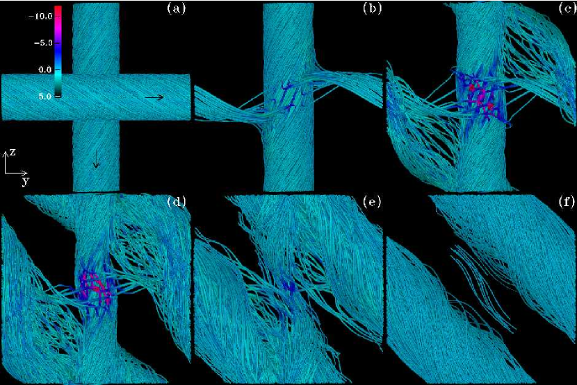
Figure 1: Fieldlines from trace particles in a slingshot reconnection. This is an RR6 collision at ${\mathcal{T}}=1$, with a uniform Lundquist number of $S_{\eta}=2880$. The color scale shows the parallel electric current, which is strongest where reconnection is occurring. The interaction is shown at $tv_{A}/R=[0,12,26,38,57,115]$.

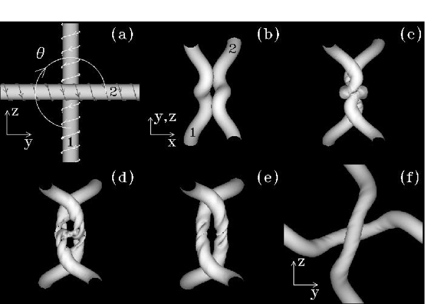
Figure 2: Isosurfaces at $|{\bf B}|_{max}/2$ from a tunnel reconnection. This is from an RR6 simulation at ${\mathcal{T}}=10$, at a uniform Lundquist number of $S_{\eta}=2880$. Flux tube 1 is parallel to the $-{\bf\hat{z}}$ axis and flux tube 2 is at an angle $\theta=6\pi/4$ relative to flux tube 1. This shows how the tubes reconnect twice to exchange center sections and tunnel. Note that the viewpoint changes from panel (a) to panel (b), and then changes back again in panel (f). The times shown are $tv_{A}/R=[0,25,42,52,61,70]$.

We focus here on two types of twisted flux tube reconnection: the slingshot and the tunnel (Dahlburg et al.,, 1997; Linton et al.,, 2001). The slingshot is simply the 3D flux tube analog of the classical 2D reconnection interaction in which two nearly straight fieldlines collide and reconnect singly with each other. A simulation of such 3D flux tube slingshot reconnection is shown in Figure 1: here a pair of cylindrical flux tubes collide at right angles to each other, and their field reconnects once at the collision site. The reconnected fieldlines ‘slingshot’ away from the collision site, releasing magnetic energy by becoming shorter, and form a new pair of cylindrical flux tubes by Figure 1(f). In contrast, as shown in Figure 2, the tunnel is a uniquely 3D phenomenon. This interaction, discovered by Dahlburg et al., (1997), starts off in Figure 2(a) in a configuration much like that of the slingshot, but rather than reconnecting just once, the flux tube fieldlines all reconnect twice, at two different places. This allows the flux tubes to exchange a small section of their volume, between the two reconnection points. Upon exchanging these sections, they reform again by Figure 2(f), but on the other side of each other from where they were initially. An analytical model developed by Linton & Antiochos, (2002) showed that the tunnel occurs because helicity conservation requires that the twist of the flux tubes decreases upon tunneling in this configuration: the reduction of twist reduces the magnetic energy, making the tunnel energetically favorable.

This paper studies the tunnel and slingshot interactions over a range of flux tube twists, collision angles, and resistive Lundquist numbers. To aid in this exploration, and to bring it into focus, we test the predictions which the analytical model of Linton & Antiochos, (2002) makes regarding these two reconnection interactions. First we test the prediction that the slingshot should transition to the tunnel as twist is increased. Second, we test the prediction that the tunnel should occur for flux tubes crossing at oblique angles as well as at right angles. In parallel with this exploration, we measure the energy released by this reconnection and compare it with the energy release predicted by the analytical model. In §2 we introduce the simulations, while in §3 and §4 we introduce the slingshot and tunnel interactions in detail. Then, in §5 we present the exploration of reconnection versus twist for the orthogonal tube collisions, as in Figures 1 and 2. In §6 and §7 we repeat this exploration for two oblique collision angles at which our theory predicts the tunnel should also occur, and we summarize our conclusions in §8.

2 Simulations

The flux tube simulations are performed with the CRUNCH3D code (see Dahlburg & Norton,, 1995), on the Cray T3E at AHPCRC and ARSC, with a grant of computer time from the DoD. This is a viscoresistive, compressible MHD code. It is triply periodic and employs a second-order Runge-Kutta temporal discretization and a Fourier collocation spatial discretization. The simulations, unless otherwise stated, are performed at a resolution of $128^{3}$ modes. The governing equations for this compressible MHD system are (as adapted from Dahlburg & Norton 1995):

$$\frac{\mbox{\unboldmath$\partial\rho$}}{\mbox{\unboldmath$\partial t$}}\mbox{\unboldmath$=-$}\nabla\cdot\mbox{\unboldmath$(\rho{\bf v}),$}$$ (1)

$$\mbox{\unboldmath$\rho$}\frac{\mbox{\unboldmath$d{\bf v}$}}{\mbox{\unboldmath$dt$}}\mbox{\unboldmath$=$}\frac{\mbox{\unboldmath${\bf J\times B}$}}{\mbox{\unboldmath$c$}}\mbox{\unboldmath$-$}\nabla\mbox{\unboldmath$p+\rho\nu$}\nabla\cdot\tau\mbox{\unboldmath$,$}$$ (2)

$$\frac{\partial{\bf A}}{\partial t}={\bf v\times B}-\frac{4\pi\eta}{c}{\bf J},$$ (3)

$$\frac{\mbox{\unboldmath$\partial E$}}{\mbox{\unboldmath$\partial t$}}\mbox{\unboldmath$=-$}\nabla\cdot\left(\frac{\mbox{\unboldmath$\rho|{\bf v}|^{2}$}}{\mbox{\unboldmath$2$}}\mbox{\unboldmath${\bf v}+$}\frac{\mbox{\unboldmath$\gamma$}}{\mbox{\unboldmath$\gamma-1$}}\mbox{\unboldmath$p{\bf v}-\kappa$}\nabla\mbox{\unboldmath$T-\nu\rho{\bf v}$}\cdot\tau\mbox{\unboldmath$+$}\frac{\mbox{\unboldmath${\bf B}$}}{\mbox{\unboldmath$4\pi$}}\times\left[\mbox{\unboldmath${\bf v\times B}$}\mbox{\unboldmath$-$}\frac{\mbox{\unboldmath$4\pi\eta$}}{\mbox{\unboldmath$c$}}\mbox{\unboldmath${\bf J}$}\right]\right)\mbox{\unboldmath$,$}$$ (4)

$$E=\frac{\rho|{\bf v}|^{2}}{2}+\frac{p}{\gamma-1}+\frac{|{\bf B}|^{2}}{8\pi}.$$ (5)

To preserve $\nabla\cdot$${\bf B}=0$, the code evolves the vector potential ${\bf A}$, with the magnetic field calculated from ${\bf B}=$$\nabla\times$${\bf A}$ whenever it is needed. Here ${\bf v}$ is the flow velocity, $p$ is the plasma pressure, $\rho$ is the density, $T$ is the temperature, $E$ is the energy density, ${\bf J}=c$$\nabla\times$${\bf B}/4\pi$ is the current, $\tau_{i,j}$ is the viscous stress tensor, $\gamma=5/3$ is the adiabatic ratio, and $c$ is the speed of light. Uniform thermal conductivity ($\kappa$) and kinematic viscosity ($\nu$) are assumed, but the magnetic resistivity ($\eta$) can have a spatial dependence.

The flux tubes we simulate here are constant twist, force free tubes, also called Gold-Hoyle flux tubes (Gold & Hoyle,, 1960). In coordinates centered on the axis of each flux tube, their magnetic field profile is

$$B_{axial}(r)=\frac{B_{0}}{1+{\mathcal{T}}^{2}r^{2}}$$ (6)

$$B_{azimuthal}(r)={\mathcal{T}}rB_{axial}(r),$$ (7)

for $0\leq r\leq R$, and the magnetic field outside the radius $r=R$ is set to zero. The twist parameter (${\mathcal{T}}$) measures the winding of fieldlines about the tube axis. Here lengths are normalized such that ${\mathcal{T}}$ measures the number of times a fieldline winds about the tube axis over $L=2\pi$ of axial distance, where $L$ is the length of the box in all three dimensions. We initialize the system with a uniform pressure inside the flux tubes of $p_{i}=20/3$ in units where the magnetic field strength on axis is $B_{0}/\sqrt{8\pi}=4$. This gives a ratio of plasma to magnetic pressure on axis of $\beta\equiv 8\pi p_{i}/B_{0}^{2}=.42$. To create pressure balance across the tube boundary, where the magnetic field drops to zero, we initialize the external pressure, $p_{e}$, to be uniform with a value:

$$p_{e}=p_{i}+\frac{B_{0}^{2}}{8\pi(1+{\mathcal{T}}^{2}R^{2})}.$$ (8)

The ideal gas law $p=\rho\mathcal{R}T$ is assumed, where $\mathcal{R}$ is the ideal gas constant. The density is initialized as $\rho=\rho_{0}p/p_{i}$, with $\rho_{0}=2$, so that the simulation volume is initially isothermal. We choose the viscosity and magnetic resistivity to be as low as possible while keeping the code stable. The viscosity is $S_{\nu}\equiv v_{A}R/\nu=2880$, and the resistive Lundquist number $S_{\eta}\equiv v_{A}R/\eta$ varies from $576$ to $288,000$. Here $v_{A}=B_{0}/\sqrt{4\pi\rho_{0}}$ is the Alfvén speed on axis, and we have chosen the flux tube radius as the typical system scale length.

Each simulation is initialized with a pair of flux tubes with axes at $x=\pm\pi/4$, where the coordinates $[x,y,z]$ each range from $-\pi$ to $\pi$. Each tube’s radius is $R=11\pi/48$, so the tubes’ fields are initially separated by a distance $\pi/24=2R/11$. Flux tube 1, at $x=-\pi/4$, always has its axial field directed along the $-{\bf\hat{z}}$ direction. Flux tube 2, at $x=\pi/4$, has its axial field aligned at an angle $\theta$ to the axis of flux tube 1, where $\theta$ is measured in the left handed sense about the ${\bf\hat{x}}$ axis, $i.e.$ in the clockwise direction from the viewpoint of Figure 2. Each configuration is represented by the notation RRX where R denotes a right handed flux tube, and $\theta=X\pi/4$. The right handed flux tube pairs shown in Figures 1 and 2 cross each other at an angle $\theta=6\pi/4$, and therefore are denoted as RR6.

This initial equilibrium is perturbed with a solenoidal velocity field, composed of two superimposed stagnation point flows, which pushes the centers of the two tubes toward each other at $x=y=z=0$:

$${\bf v}(x,y,z)=v_{0}[-\sin{x}(\cos{y}+\cos{z})~{}{\bf\hat{x}}+\cos{x}(\sin{y}~{}{\bf\hat{y}}+\sin{z}~{}{\bf\hat{z}})].$$ (9)

This is not a driven flow, but rather is initialized at the start of the simulation, with an amplitude $v_{0}=v_{A}/40$, and then evolves dynamically as prescribed by the momentum equation (eq. 2).

The helicity of the simulation is calculated via

$${\mathcal{H}}=\int{\bf A\cdot B}dV,$$ (10)

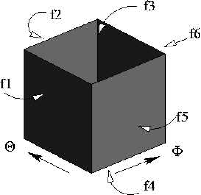
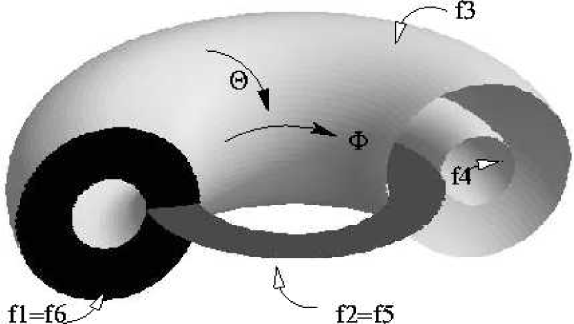
Figure 3: Sketch of the toroidal mapping of a doubly periodic volume. In the mapping, surface $f1$ is joined to surface $f6$ while surface $f2$ is joined to surface $f5$. If no flux penetrates the boundaries of the toroidal volume, then the helicity is simply ${\bf A\cdot B}$ integrated over the volume.

where the integral is taken over the volume of the simulation. Hornig, (2005) shows that the helicity can be calculated in this simple manner for a triply periodic box on the condition that magnetic flux penetrates at most two of the three sets of boundaries. In that case, the periodic box can be mapped to a volume enclosed within a pair of toroidal shells, as sketched in Figure 3, so that no flux leaves the closed volume. For example, if in Figure 3 flux penetrates the periodic side boundaries of the cube at $f1=f6$ and $f2=f5$ but not $f3=f4$, then $f1$ can be wrapped around to meet $f6$ and $f2$ can be wrapped around to $f5$, forming the toroidal domain shown on the right. The result is that the flux penetrating these boundaries never leaves the toroidally mapped volume. Thus, in such a mapping, the helicity is well defined. A necessary constraint on this formulation is that no flux thread the torus outside the simulation volume (see Hornig,, 2005). This means that no flux can thread the volume poloidally through the ‘donut hole’ (through the area inside the grey ring), and no flux can thread it toroidally along the innermost torus (through the area inside the black ring). To ensure this, the gauge for ${\bf A}$ is chosen so that the integrals of the vector potential along the lines around the outer edges of these areas, i.e. along the intersection of boundary $f1$ with $f4$ and of boundary $f2$ with $f3$, are zero:

$$\oint_{f1\bigcap f4}{\bf A\cdot dl}=0=\oint_{f2\bigcap f3}{\bf A\cdot dl}.$$ (11)

A consequence of this choice of mapping and gauge is that when a pair of untwisted flux tubes cross as in Figure 1 with a horizontal tube on the positive $x$ side of a vertical tube, the tubes do not link each other in the toroidal mapping, and so have a helicity of zero. If the $x$ positions of the tubes are switched, they do link each other in the mapping, and so have a linking number ${\mathcal{L}}={\mathcal{H}}/\Phi^{2}=2$, where $\Phi$ is the axial magnetic flux per flux tube. Additionally, a single untwisted flux tube crossing the domain diagonally in the ${\bf\hat{y}}+{\bf\hat{z}}$ direction will have a helicity of ${\mathcal{H}}/\Phi^{2}=-1$, whereas a flux tube crossing on the orthogonal diagonal will have a helicity of ${\mathcal{H}}/\Phi^{2}=1$. Taking this into account, we have verified that the simulation calculates the correct helicity for each of the simulations reported here, and we can track the evolution of the helicity during the flux tube interactions. These values for the helicity can be different from what is obtained from calculating the relative helicity with respect to a potential reference field (e.g. Berger & Field,, 1984; Finn & Antonsen,, 1985), but the meaningful measures are the change in total, crossing, and twist helicity from one state to another, and these are the same under both formalisms. The first advantage of this toroidal mapping method is that it is much simpler to implement. The second advantage is that it is uniquely defined for triply periodic domains wherein a net magnetic flux crosses only two of the three sets of boundaries, as is the case for our simulations. In contrast, Berger, (1987) showed that the relative helicity formulation of Berger & Field, (1984) and Finn & Antonsen, (1985) is not in general uniquely defined for triply periodic domains unless no net magnetic flux crosses any of the boundaries.

3 Slingshot Reconnection

We will now discuss the slingshot interaction shown in Figure 1 in more detail, and address an issue this simulation brings up regarding the use of a periodic vector potential to calculate the magnetic field. Figure 1 shows the interaction of RR6 tubes with a twist of ${\mathcal{T}}=1$ at a uniform Lundquist number of $S_{\eta}=2880$. Figure 1(a) shows the initial configuration: the fieldlines of both tubes are displayed, and one can see that they are both right handed and wind about the tube axes once over the length of the simulation box. These fieldlines are traced from four $16^{2}$ grids of trace particles initially placed near both ends of both flux tubes. As the simulation progresses, these points move dynamically subject to the momentum equation (eq. [2]). To the extent that the fieldlines are frozen into the flow, this allows us to follow the dynamics of fieldlines. Subsequently, in Figures 1(b) through 1(f), only fieldlines traced from the trace particles initially on the vertical flux tube are shown. This allows the reconnection region between the tubes to be seen in the figure. In addition, it makes reconnected fieldlines stand out: fieldlines connecting to the horizontal boundaries are visible only if they have reconnected and are attached to the vertical flux tube. Figure 1(b) shows the reconnection starting at the point where the two tubes first come into contact. The reconnected fieldlines form a sharp angle near the reconnection region, because the slingshot action of these fieldlines has not yet pulled them away from the reconnection region. By Figure 1(c) the tension force has snapped these fieldlines away from the site of their reconnection, converting magnetic energy into kinetic energy, which then diffuses away via viscous drag. This reconnection and snapping away continues through Figures 1(d) and 1(e) until, by Figure 1(f), all of the field has reconnected to form a new pair of flux tubes. Throughout this figure, the parallel electric current $J_{\parallel}={\bf J\cdot B}/|{\bf B}|$ is shown by the color, with bright red being the strongest (negative) parallel current as shown by the color bar. The values of parallel current are normalized here by the initial current on axis $J_{0}=cB_{0}/(2\pi{\mathcal{T}})$. Parallel currents are a key signature of 3D reconnection (Schindler et al.,, 1988), and so this color highlights the regions of strong reconnection, which are particularly evident in Figures 1(c) and 1(d).

As the wavelength of the twist is significantly longer than the length of the collision interface, this reconnection should closely resemble the reconnection of untwisted flux tubes. Indeed, locally, the field does reconnect in the straightforward fashion one expects from untwisted reconnection. But there is a significant difference here from the untwisted reconnection simulated by Linton & Priest, (2003). In the untwisted simulations, the flux tubes flatten out on contact and break up into several pieces so that only a fraction of the flux reconnects. Here, in contrast, even this small amount of twist is strong enough to keep the tubes from flattening out and breaking up, so that all of the flux reconnects to form a new pair of isolated flux tubes. Thus, the twist does not alter the local, relatively small scale dynamics of the reconnection region, but it does act on the large scale dynamics of the flux tubes to keep them coherent throughout the reconnection process, and so changes the global reconnection in a fundamental way.

Note that the reconnection seen here apparently contradicts the reconnection results reported by Dahlburg et al., (1997). They found that the collision of flux tubes in an apparently identical configuration, RR6 with ${\mathcal{T}}=1$ and the same Lundquist number we use here, results in little or no reconnection: instead, the tubes bounce off each other. The resolution of this contradiction is that the initial conditions for their simulation have a small amount of background field, which interferes with the reconnection at small twist. This background field arises naturally from the periodic boundary conditions on the magnetic vector potential A. Such a periodic vector potential can represent a periodic magnetic field ${\bf B}=$$\nabla\times$${\bf A}$, but it allows no net magnetic flux in any direction. Formally, the net flux in, for example, the ${\bf\hat{z}}$ direction is the integral of $\bf{A}$ on the curve running around the edge of the simulation box at any value of $z=z_{c}=const$:

$$\Phi_{z}=\oint_{z_{c}}{\bf A\cdot dl}=\int_{-\pi}^{\pi}A_{x}|_{y=-\pi}dx+\int_{-\pi}^{\pi}A_{y}|_{x=\pi}dy+\int_{\pi}^{-\pi}A_{x}|_{y=\pi}dx+\int_{\pi}^{-\pi}A_{y}|_{x=-\pi}dy.$$ (12)

Since the periodic boundary conditions mean that $A_{y}(-\pi,y,z_{c})=A_{y}(\pi,y,z_{c})$ and $A_{x}(x,-\pi,z_{c})=A_{x}(x,\pi,z_{c})$, the two $dy$ integrals cancel each other, as do the two $dx$ integrals, and so there must be no net flux in the ${\bf\hat{z}}$ direction. Instead, the magnetic field which results from a periodic vector potential is the specified field plus a uniform background field whose net flux exactly cancels the net flux of the specified field. To correct for this background field effect, we calculate ${\bf B}$ at each step as

$$\mbox{\unboldmath${\bf B}=$}\nabla\times\mbox{\unboldmath${\bf A}+B_{0x}{\bf\hat{x}}+B_{0y}{\bf\hat{y}}+B_{0z}{\bf\hat{z}}$}$$ (13)

where the three background field constants are calculated at the start of the simulation, when the ${\bf B}$ field is specified, as

$$B_{0i}=\int_{-\pi}^{\pi}\int_{-\pi}^{\pi}\frac{{\bf B}|_{x_{i}=const}}{4\pi^{2}}{\bf\cdot\hat{x}_{i}}dx_{j}dx_{k}.$$ (14)

These corrections are then saved for use during the rest of the simulation, and A is calculated from the inverse laplace transform of B:

$$\nabla\times\mbox{\unboldmath${\bf B}=$}\nabla\times\nabla\times\mbox{\unboldmath${\bf A}=\nabla^{2}{\bf A},$}$$ (15)

$$\mbox{\unboldmath${\bf A}=$}\nabla\times\frac{\mbox{\unboldmath$1$}}{\mbox{\unboldmath$\nabla^{2}$}}\mbox{\unboldmath${\bf B}.$}$$ (16)

From then on, ${\bf A}$ is evolved dynamically by the code, ensuring that the solenoidality of ${\bf B}$ is preserved.

An obvious question that this formalism raises is: does the lack of any presence of the background field in the periodic vector potential affect the dynamics? Only the induction equation could be affected, as the other dynamical equations rely on ${\bf B}$ to calculate magnetic effects rather than ${\bf A}$. Fortunately, the induction equation,

$$\frac{\partial{\bf A}}{\partial t}={\bf v\times B}-\frac{4\pi\eta}{c}{\bf J},$$ (17)

can also be shown to be unaffected by the absent linear component of ${\bf A}$. Both the source terms ${\bf J}$ and ${\bf v\times B}$ make no linear contribution to this equation, as ${\bf J}$, ${\bf v}$, and ${\bf B}$ are all periodic in space, and so have no linear components. Thus the linear part of the induction equation is reduced to $\partial{\bf A}_{linear}/\partial t=0$, which just confirms our assumption that ${\bf A}_{linear}$ and therefore the background magnetic correction terms $B_{0i}$ are constant in time. Note that the helicity calculation of equation (10) is the one place where the linear corrections to the vector potential are needed: for this integral the correction ${\bf A}_{linear}={\bf\hat{y}}B_{0z}x-{\bf\hat{z}}B_{0y}x$ are therefore added to ${\bf A}$ (assuming that $B_{0x}=0)$.

We have carefully checked the resulting magnetic field, and found that it matches our input conditions. We have also checked the field without this correction and found that there is indeed zero net flux in all directions. The correction has been included in the simulations reported here, in Linton et al., (1998, 1999, 2001), and in Linton & Priest, (2003), but not in the simulations performed by CRUNCH3D before that time. Thus for the Dahlburg et al., (1997) simulations, with flux tubes directed in the $-{\bf\hat{z}}$ direction and in the ${\bf\hat{y}}$ direction, there is an extra background field directed diagonally across the whole simulation volume in the $-{\bf\hat{y}}+{\bf\hat{z}}$ direction. The ${\bf\hat{z}}$ background component, for example, is

$$B_{z0}\equiv\frac{\int B_{z}dxdy}{\int dxdy}=\frac{\pi B_{0}\ln(1+{\mathcal{T}}^{2}R^{2})}{{\mathcal{T}}^{2}L^{2}}.$$ (18)

For ${\mathcal{T}}=1$ this gives $B_{z0}=.13$ versus a peak axial field strength in the flux tube of $B_{0}=4$. A part of this field lies between the tubes and so provides a force to block them from coming in contact. We have performed this simulation with this correction turned off, and replicated the flux tube bounce seen by Dahlburg et al., (1997). We then turned the correction on and found the slingshot interaction shown in Figure 1 and discussed above. Note that for ${\mathcal{T}}=10$, equation (18) this gives $B_{z0}=.013$, so the effect is weaker in that case than in the low twist case, likely explaining why the flux tubes reconnected at ${\mathcal{T}}=10$ to tunnel in Dahlburg et al., (1997) in spite of the background field.

4 Tunnel Reconnection

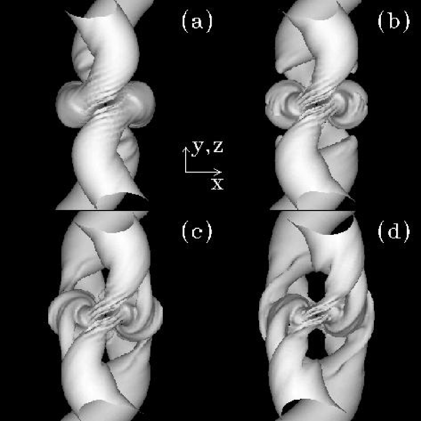
Figure 4: Closeup view of Figure 2 at $tv_{A}\pi/R=[42,47,49,52]$.

Having introduced the slingshot reconnection, we will now introduce the tunnel reconnection, and discuss the theory of why it occurs. Figure 2 shows isosurfaces at $|{\bf B}|=|{\bf B}|_{max}/2$ for a simulation of an RR6 collision at ${\mathcal{T}}=10$, a uniform resistivity of $S_{\eta}=2880$, and at a resolution of $256^{3}$. Figures 2(a) and 2(f) show the beginning and end of the simulation from the same viewpoint (from the ${\bf\hat{x}}$ axis). These panels show that, as seen by Dahlburg et al., (1997), the flux tubes reconnect such that they tunnel entirely through each other. To make the reconnection more visible, the intermediate panels show the interaction as seen from the upper left hand corner of the view shown in Figure 2(a). In Figure 2(b) the tubes have just collided, and are rebounding, exciting the helical kink instability. Figure 2(c) shows that, before they can completely rebound, the tubes start to reconnect at two places. To show the reconnection in more detail, the center of Figure 2(c) is shown in a closeup view in Figure 4(a), along with a closeup of Figure 2(d) in Figure 4(d) and a closeup of two intervening time steps in Figures 4(b) and 4(c). The two tubes reconnect on the near side and the far side of this view. The bulging sections of flux tube (to the left and right of the center of the collision) between the reconnection points do not appear to reconnect: they remain in evidence throughout Figures 4(a)-4(d). However, as the reconnection proceeds, the connections to these sections change dramatically. In Figures 4(a) and 2(c), the near flux tube at the bottom is attached to the bulging section on the right, and then to the far flux tube at the top of the simulation. But by Figures 4(d) and 2(d), the near flux tube at the bottom is attached to the left bulging section and then, as before, to the far flux tube at the top. So the top and bottom parts of this flux tube are the same as at the beginning, but the middle section has been exchanged with that of the other flux tube, resulting in a change of position of the two flux tubes. In this manner, the flux tubes appear to tunnel through each other. Note that the inverse reaction, where tubes in the configuration of 2(f) collide with each other, does not result in a tunnel. Linton et al., (2001) simulated this RR2 collision and found that, at a twist of ${\mathcal{T}}=10$, the flux tubes simply bounce off each other. This tunnel interaction therefore raises two questions: 1) why does it occur and 2) why is it not reversible?

To address these questions, Linton & Antiochos, (2002) explored the tunneling interaction analytically, assuming helicity conservation, and using the concepts of magnetic twist and linking or crossing number developed by Berger & Field, (1984). They found a promising explanation: by tunneling, flux tubes change how they link each other, as measured by the linking number ${\mathcal{L}}$ (see Wright & Berger,, 1989). As mentioned earlier, for the helicity formalism we use here, the flux tubes in Figure 2(a) have ${\mathcal{L}}=0$, wheres those in Figure 2(f) have ${\mathcal{L}}=2$. Thus in tunneling, their linking number increases by $2$. Note that in any another helicity formalism, the value of ${\mathcal{L}}$ may be different, but the change in ${\mathcal{L}}$ due to reconnection, which is the only meaningful number, will be exactly the same as it is in this formalism. The sum of the tubes’ linking and twist numbers is their total helicity, ${\mathcal{H}}/\Phi^{2}=2{\mathcal{T}}+{\mathcal{L}}$, and this sum must be conserved to conserve helicity. When the tubes tunnel to increase their linking helicity, their twist helicity must decrease. For an RR6 configuration tunneling to RR2, the positive twist ${\mathcal{T}}$ is reduced by one turn per flux tube upon tunneling, and the twist energy decreases as ${\mathcal{T}}^{2}$. In the opposite interaction, when RR2 flux tubes tunnel to an RR6 configuration, the linking number decreases by $2$, and so the twist must increase by one turn per tube, increasing the magnetic energy. This inverse reaction is energetically unfavorable, and therefore not expected to occur, in agreement with the simulation results of Linton et al., (2001).

Linton & Antiochos, (2002) found that the magnetic energy, normalized by $4{\mathcal{T}}^{2}/(LB_{0}^{2})$, of the pair of Gold-Hoyle flux tubes we simulate here is initially

$$M_{0}=(1+\zeta)(\Gamma_{12}+\Gamma_{32})$$ (19)

where $L\zeta$ is the length of flux tube 2 in the simulation box. When this tube crosses the box perpendicular to the boundaries, as in RR6, its length is $L$, the same as the length of flux tube 1, and so $\zeta=1$. When this tube crosses the box at a diagonal, as in RR5 or RR7, its length is $\sqrt{2}L$ and $\zeta=\sqrt{2}$. The constants $\Gamma_{12}$ and $\Gamma_{32}$ come from integration of the square of the initial axial (eq. [6]) and azimuthal (eq. [7]) magnetic field, respectively, over the tube cross section, and have the form

$$\Gamma_{12}=\frac{{\mathcal{T}}^{2}R^{2}}{2+2{\mathcal{T}}^{2}R^{2}}$$ (20)

and

$$\Gamma_{32}=\frac{1}{2}\left(\ln(1+{\mathcal{T}}^{2}R^{2})-\frac{{\mathcal{T}}^{2}R^{2}}{2+2{\mathcal{T}}^{2}R^{2}}\right).$$ (21)

From helicity conservation along with mass and flux conservation, flux tubes initially crossing at angles in the range $\pi<\theta<2\pi$ should have a normalized magnetic energy after tunneling of

$$M_{t}=(1+\zeta)\Gamma_{12}+\left(\frac{({\mathcal{T}}\zeta-1)^{2}}{{\mathcal{T}}^{2}\zeta}+\frac{({\mathcal{T}}-1)^{2}}{{\mathcal{T}}^{2}}\right)\Gamma_{32}.$$ (22)

Here the factors ${\mathcal{T}}\zeta-1$ and ${\mathcal{T}}-1$ take account of the loss of $1$ turn of twist in each flux tube due to tunneling. Note that this result relies on the assumption that the tubes evolve homologously: $i.e.$ that are they still uniform twist tubes after reconnection. This equation shows that the tunnel changes the azimuthal energy ($\propto\Gamma_{32}$) but not the axial energy ($\propto\Gamma_{12}$). Linton & Antiochos, (2002) applied the same analysis to the slingshot tubes: in that case, the tubes lose only $1/2$ turn of twist as they reconnect. However, the axial field can also lose energy because the slingshot allows the tubes to shorten, as shown in Figure 1. They find that these tubes should have a normalized magnetic energy after slingshot of

$$M_{s}=\frac{4}{\zeta+1}\frac{L_{s}^{2}}{L^{2}}\Gamma_{12}+2\frac{L}{L_{s}}\frac{1}{{\mathcal{T}}^{2}}\left({\mathcal{T}}\frac{\zeta+1}{2}-\frac{1}{2}\right)^{2}\Gamma_{32},$$ (23)

where $L_{s}$ is the length of the tube after slingshot. Here the factor ${\mathcal{T}}(\zeta+1)/2-1/2$ accounts for the loss of $1/2$ turn of twist per flux tube in a slingshot.

If we assume that flux tubes will reconnect in the manner which releases the most energy, we can now predict whether a given colliding flux tube pair will slingshot or tunnel when they reconnect. For this analysis, we use the optimal slingshot length $L_{s}$ in calculating the slingshot energy, as in Linton & Antiochos, (2002) equation (40). This length is calculated to be that which gives the lowest slingshot energy, given the geometrical constraint that the length cannot be shorter than the distance between the tube’s footpoints. This optimal length is not always the shortest because, as shown by equation (23), the axial field energy of the tubes (the $\Gamma_{12}$ term) varies as $L_{s}^{2}$ while the azimuthal energy (the $\Gamma_{23}$ term) varies as $1/L_{s}$. The optimal length is therefore a compromise between axial and azimuthal (twist) energy.

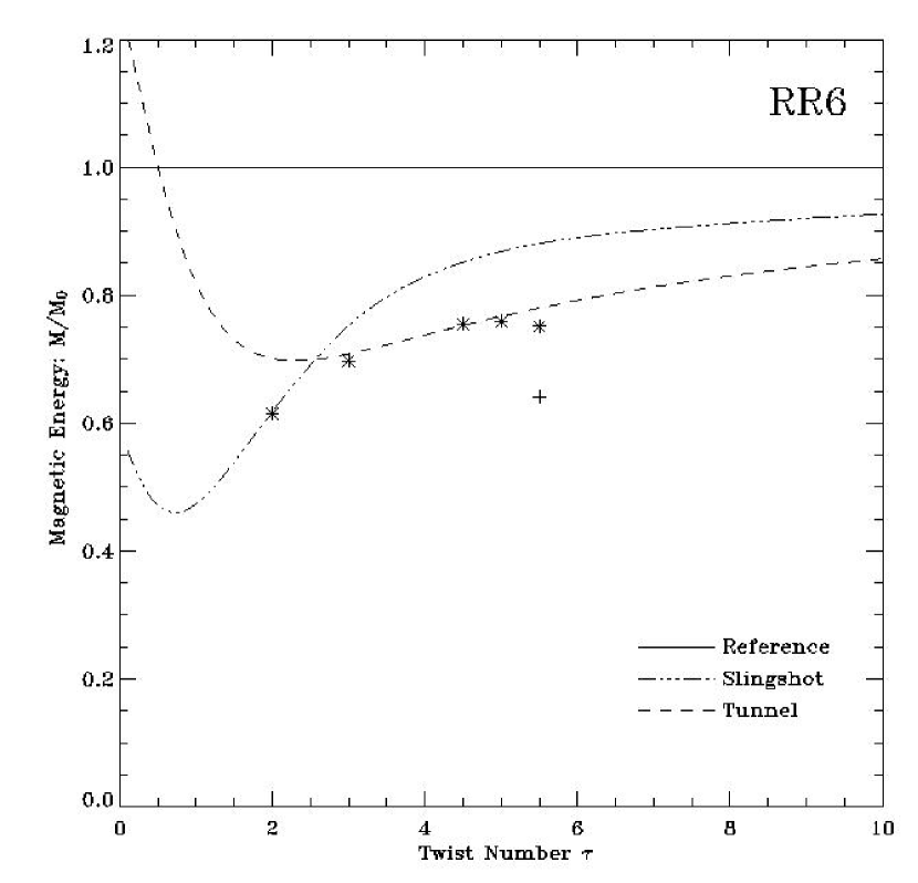
Figure 5: Theoretical reconnection energy for RR6 simulations at various twists. The dashed line shows the predicted tunnel energy, as calculated from equation (22), and the dash-triple-dot line shows the slingshot energy, as calculated from equation (23). The asterisks denote simulation values for slingshot interactions, while the plus sign denotes the simulation value for the tunnel interaction of Figure 7. All the simulation data shown here is from the nonuniform resistivity calculations, with a background, maximum Lundquist number of $L_{\eta}=288,000$.

We plot the predicted energies from this analysis as a function of twist for these two reconnected states, normalized by the initial state, in Figure 5 for the RR6 collision. The resulting slingshot and tunnel energy curves are shown by the dashed-triple-dotted and by the dashed curves, respectively. The tunneled state is at a lower energy for high twists, because the twist energy dominates in that regime, and the tunnel releases more twist energy than the slingshot. The slingshot state, in contrast, is at lower energy for low twist, as the axial field energy dominates there, and the slingshot can release axial energy by making the tubes shorter, whereas the tunnel cannot. These two curves cross at ${\mathcal{T}}=2.56$, predicting that at twists below this level the slingshot loses more energy than the tunnel. If energy release alone dictates the resulting state, the interaction should be a slingshot reconnection below that twist and a tunnel above that twist. Obviously the dynamics between the beginning and end state will play an important role, but the expected energy release given by equations (22) and (23) should provide a useful predictor of the end state.

Do the simulations agree with these predictions? In Figure 1 we show that the slingshot occurs at ${\mathcal{T}}=1$ and $S_{\eta}=2880$, and in Figure 2 we show that the tunnel occurs at ${\mathcal{T}}=10$ and $S_{\eta}=2880$, so, in agreement with our theory, there is clearly a transition at some level of twist between $1$ and $10$. However, Dahlburg et al., (1997) also found that the type of reconnection which occurs depends on the Lundquist number: for ${\mathcal{T}}=10$ RR6 flux tubes, they found that at $S_{\eta}=2880$ a tunnel occurs, but at $S_{\eta}=576$ a slingshot occurs. Clearly there is a dependence on resistivity as well as twist. In the following section, we will present a series of MHD simulations testing these analytical predictions for the transition as a function of twist, and will also explore the dependence of the transition on resistivity.

5 RR6 Reconnection

For our first set of RR6 simulations, we searched for the transition from tunnel to slingshot reconnection as a function of twist at four different spatially uniform Lundquist numbers. At the lowest number we tested, $S_{\eta}=576$, we found only slingshot interactions even at twists as high as ${\mathcal{T}}=14$. This agrees with the finding by Dahlburg et al., (1997) that a ${\mathcal{T}}=10$ collision at this Lundquist number results in a slingshot. It also suggests that, since the tubes slingshot even at very high twist, the tunnel will never occur for any twist at such a low Lundquist number. However, by increasing the Lundquist number to $1440$, we did find that the tubes tunnel at twists equal to or greater than $6.5$. Below this critical value, at twists equal to or below $6$, the slingshot occurs. Note that our resolution in twist is only $\delta{\mathcal{T}}=.5$, as an entire flux tube collision simulation is necessary for each data point, so high resolution in ${\mathcal{T}}$ space is expensive. Clearly at moderate Lundquist numbers both the tunnel and slingshot can occur, though the transition from one to the other occurs at a significantly higher level than the prediction of ${\mathcal{T}}=2.56$ from the analytical model. As we increased the Lundquist number from $1440$, the critical twist for the transition decreased: the tunnel occurs down to a twist of $6$ at a Lundquist number of $2880$ and to a twist of $5.5$ at a Lundquist number of $5760$. We postulated that this decrease in critical twist as a function of Lundquist number is because the twist diffuses away due to the resistivity: the lower the Lundquist number, the faster the twist disappears during the simulation. In effect, enough twist may disappear before the tubes have a chance to tunnel that the tubes see a much lower level of twist than the code was initialized with. In fact, for the ${\mathcal{T}}=5.5$ tunnel simulation at $S_{\eta}=5760$ the helicity decreases to $53\%$ of its initial value by the time the tubes finish tunneling. As the linking number is zero in this configuration, the helicity is purely due to the twist, and so this indicates that the twist per tube diffuses from $5.5$ to $2.9$ during that time. At the very low Lundquist number of $576$, twist would diffuse away at an even faster rate. Thus it is not surprising that the tubes do not tunnel at such a low Lundquist number even if their initial twist is very high.

As the code becomes unstable at Lundquist numbers higher than $5760$ for these simulations, we could not decrease the resistivity further to see if the transition eventually goes to the predicted level of ${\mathcal{T}}=2.56$ as the Lundquist number gets very large. Instead we turned to the possibility of a nonuniform resistivity. We modified the code so that it has a ball of high resistivity at the center of the simulation box, where the flux tubes collide, of the form

$$\eta=\eta_{0}(1+99e^{-\lambda^{2}/(4R^{2})}),$$ (24)

where $\lambda$ is the radial distance from the center of the box: $\lambda=(x^{2}+y^{2}+z^{2})^{1/2}$. The diameter ($2R$) of the flux tubes is used as the scale length so that the collision area of the tubes will mostly be within the high diffusion area. This ensures that the region of intense dynamics has sufficient diffusion that the reconnection does not destabilize the code, but allows the majority of the flux tubes’ volume, which is well away from the reconnection, to diffuse at a much slower rate. This worked very well, and we were able to run the code at a background Lundquist number of $288,000$, with a minimum Lundquist number in the collision region of $2880$. In this case, tubes at ${\mathcal{T}}=5.5$ tunnel in about $1/5$ the time it takes them to tunnel at a uniform resistivity of $S_{\eta}=5760$, and the helicity only decreases by $6\%$. This indicates two important results. First, the loss of helicity is clearly due to diffusion rather than to reconnection, as both the high and low Lundquist number simulations undergo the same tunnel reconnection, but the low Lundquist number simulation loses about $8$ times more helicity than the high Lundquist number simulation. Second, at a loss of only $6\%$, the twist is reduced from $5.5$ to $5.2$ due to diffusion. This difference is well below our resolution of $\delta{\mathcal{T}}=.5$, and so diffusive loss of twist should have a negligible effect on the tunnel to slingshot transition. We still found, however, that the tubes tunnel only down to a twist of $5.5$ and then slingshot for twists of $5$ and below. The true simulation limit at which the tunnel can occur for an RR6 collision therefore appears to be in the range ${\mathcal{T}}=5$ to $5.5$, as opposed to the analytical prediction of $2.56$.

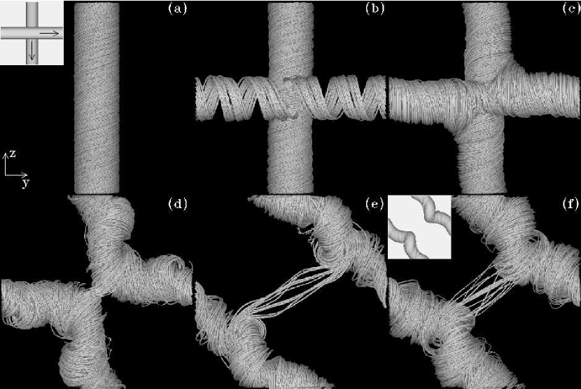
Figure 6: Fieldlines from the RR6 simulations at ${\mathcal{T}}=5$ and for the nonuniform Lundquist number with a maximum of $288,000$. At this level of twist the tubes slingshot. The panels shown here are at times $tv_{A}/R=[0,14,27,45,85,194]$.

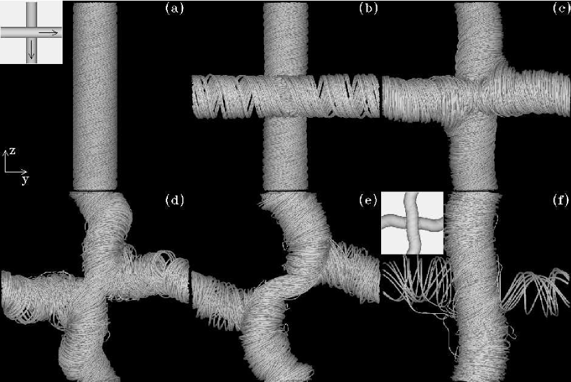
Figure 7: Fieldlines from simulation RR6 at ${\mathcal{T}}=5.5$ and for a nonuniform Lunquist number with a maximum of $288,000$. At this level of twist the tubes tunnel. The panels shown here are at times $tv_{A}/R=[0,14,28,46,79,159]$.

Figures 6 and 7 show the simulations on either side of this transition from tunnel to slingshot for these nonuniform resistivity simulations with $S_{\eta}=288,000$ outside the collision region. Figure 6 shows the ${\mathcal{T}}=5$ simulation: as before, only the fieldlines from the trace particles in the vertical tube are plotted. The inset in Figure 6(a) shows the initial tube isosurfaces at $|{\bf B}|=|{\bf B}|_{max}/3$, with arrows superimposed on the tubes to show the axial field directions. The field from the tubes reconnects in Figures 6(b) through 6(d), and slingshots in Figures 6(e) and 6(f) to form a pair of diagonal, reconnected tubes. An isosurface of the field in the final state is inset into Figure 6(f) for comparison with the initial state in Figure 6(a): clearly the tubes have slingshot to a shorter length, though the twist remaining after reconnection is strong enough to kink the tubes into a helical shape. The majority of the fieldlines simply slingshot because they only reconnect once, but Figures 6(e) and 6(f) show a small number of fieldlines which have reconnected twice to tunnel. These fieldlines connect the slingshotted tubes at their centers and exert a tension force pulling the reconnected tubes back together. However this force is insufficient to bring the tubes close enough that they come in contact again: by Figure 6(f) the configuration has settled into a static equilibrium, and the interaction is over. Presumably, if the tubes had been pulled back into contact, their fieldlines would have reconnected again to tunnel to the lower energy state. This shows the limitations of the energy analysis: if the barrier to tunnel reconnection is too large to overcome, as for example, when the tubes do not remain in contact long enough for the fieldlines to reconnect twice, the tubes will not tunnel.

Figure 7 shows the ${\mathcal{T}}=5.5$ RR6 flux tube interaction. Most of the interaction is very similar to the ${\mathcal{T}}=5$ interaction, as one would expect, considering how small a difference in twist there is between the two simulations. The tubes reconnect in Figures 7(b) through 7(d) and start to slingshot in Figure 7(e). However, more of the fieldlines have reconnected twice to tunnel by this point than in the ${\mathcal{T}}=5$ simulation. When the tension force of these fieldlines pulls the tubes back toward each other, they actually bring the tubes into contact again. The tubes can therefore reconnect a second time to tunnel by Figure 7(f). The majority of the horizontal fieldlines are no longer plotted by Figure 7(f) because they are no longer connected to the vertical tube as they were in the preceding panels: the horizontal tube has been recreated with little or no connection to the vertical tube. The isosurface inset into Figure 7(f) clearly shows that the field of this recreated horizontal flux tube is now behind the field of the vertical flux tube, in contrast to the initial state of Figure 7(a), where it was in front. The fact that these tubes attempt to slingshot in Figure 7(e) before recombining to tunnel confirms our conjecture in the previous paragraph: the slingshot flux tubes must be pulled back into contact again after their first reconnection if they are to reconnect a second time and tunnel to the lowest energy state.

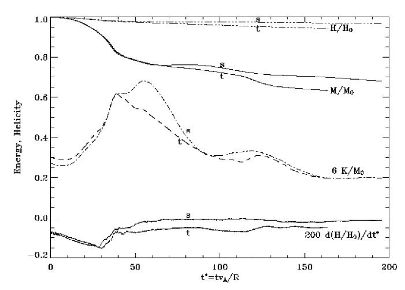
Figure 8: Time evolution of helicity, magnetic energy, kinetic energy, and time derivative of helicity for the RR6 ${\mathcal{T}}=5.5$ tunnel simulation (t) and for the RR6 ${\mathcal{T}}=5$ slingshot simulation (s).

Figure 8 shows the energetics of these two interactions. From top to bottom, we plot the helicity (dash-triple-dot lines), the magnetic energy (solid lines), the kinetic energy (dashed and dash-dot lines), and the time derivative of helicity (solid lines). In each case, the slingshot and tunnel lines are labeled with ‘s’ and ‘t’, respectively. A large peak in the kinetic energy at about $tv_{A}/R=40$, accompanied by a significant drop in the magnetic energy shows that the slingshot reconnection is converting magnetic into kinetic energy in both simulations at this time. After this point, the ${\mathcal{T}}=5$ tubes, which only slingshot, continue to convert magnetic into kinetic energy and reach an even higher kinetic energy peak at just after $tv_{A}/R=50$. Once the reconnection is over, the kinetic energy starts to drop. This is partly due to viscous losses, but also due to harmonic oscillation of the flux tubes: they overshoot their new optimal equilibrium positions, and slow to a stop as the magnetic fields are overstretched. Thus this drop in kinetic energy at $tv_{A}/R=80$ to $90$ is accompanied by a brief rise in the magnetic energy. The tubes then rebound, briefly increasing their kinetic energy again before they settle into an equilibrium. During this period, the magnetic energy of the tunneling tubes at ${\mathcal{T}}=5.5$ also steadily decreases due to diffusion until the tubes come into contact again at about $tv_{A}/R=110$. Then the reconnection starts again as the tubes tunnel: the magnetic energy decreases at a faster rate than it did during the preceding diffusion stage, and the kinetic energy shows another local peak. This peak is, however, significantly lower than the peak from the slingshot reconnection in either simulation, as the tunnel is much less dynamically active than the slingshot.

The helicity decreases very slowly during the whole simulation, but the time derivative of helicity shows that the helicity decay rate increases linearly for the first $30$ Alfvén times. This is likely due to the increase in magnetic gradients between the flux tubes during this interval, as the two tubes collide and generate a current sheet between them. Next, from $tv_{A}/R=30$ to $tv_{A}/R=40$, the helicity decay rate slows rapidly, and then it settles down to a nearly constant rate for the rest of the simulation. The slowdown is likely due to the destruction by reconnection of the sharp magnetic gradients induced by the initial collision. For the remainder of the simulation, the slingshot helicity decays at a slower rate than the tunnel helicity: this is likely because the slingshot removes the tubes entirely from the central, high diffusion region while the tunnel keeps the tubes near that region for the entire interaction, so the tunnel tubes see a higher average resistivity and decay at a faster rate.

In addition to measuring the twist at which the RR6 interaction transitions from tunnel to slingshot, we can also measure the energy release for each interaction, and compare that with the value predicted by the analytical theory in Figure 5. By studying the time sequence of the fieldline plots during the ${\mathcal{T}}=5.5$ tunnel reconnection, we estimate that the slingshot and subsequent rebound reaches its end state at $tv_{A}/R=72$, at which point $25\%$ of the magnetic energy has been lost. This can be compared with a prediction by the analytical theory of a loss of $12\%$ due to a slingshot. Similarly, at $tv_{A}/R=151$ the tunnel appears to be complete, at which point a total of $36\%$ of the magnetic energy has been lost to reconnection and diffusion, compared to a predicted loss of $22\%$ due to a tunnel reconnection. These values, and the equivalent values for the other simulations we performed at this high Lundquist number, are plotted in Figure 5 as asterisks for slingshots and as plus signs for the tunnel. Note there are both a tunnel and slingshot energy value for the ${\mathcal{T}}=5.5$ simulation, as we saw both interactions in that case. As magnetic energy is being released via diffusion during the entire simulation, as well as via the reconnection, we expect that more magnetic energy will be lost than is predicted by the analytical theory for reconnection alone. One can see from Figure 5 that this is true. The actual energy release for the slingshot is very close to the predicted value for ${\mathcal{T}}=2$ but increases gradually until about twice the predicted amount is released at ${\mathcal{T}}=5$. This makes sense, as the slingshot occurs more quickly at low twist, where there is no hint of a tunnel, than at high twist, where there is a battle between the slingshot and tunnel which slows the interaction down. So at high twist, there is more time for the field to lose energy to diffusion before the interaction is complete.

A second possible reason for the extra energy release in the simulations relative to what is predicted by the theory is that the flux tubes may not evolve homologously to a uniform twist configuration after reconnection, but may instead evolve to a lower energy state. Taylor, (1986) showed that the lowest energy state a twisted field can evolve to while conserving total helicity is a constant $\alpha$ force free state, where

$$\alpha\equiv\frac{{\bf J}\cdot{\bf B}}{|{\bf B}|^{2}}.$$ (25)

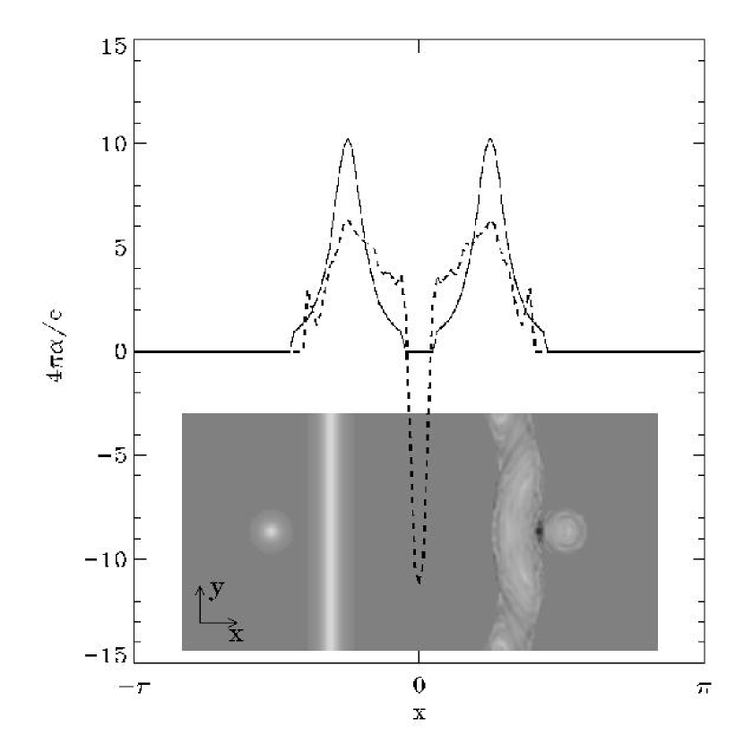
Figure 9: Plot of $\alpha$ for the RR6 tunnel simulation of Figure 7. The solid line shows the initial state ($tv_{A}/R=0$) at $y=z=0$, while the dashed line shows the final, tunneled state (at $tv_{A}/R=159$). The inset greyscale plots show $\alpha$ at the same times in the $z=0$ plane, where the left plot is the initial state and the right plot is the final state. Here black is $4\pi\alpha/c=-15$ and white is $4\pi\alpha/c=15$. This shows that the two tubes evolve towards constant $\alpha$ fields during their reconnection.

The reconnection which occurs here gives the fields the opportunity to evolve towards this state. Figure 9 shows $\alpha$ for the initial and final states of this simulation, measured for $|{\bf B}|^{2}>|{\bf B}|^{2}_{max}/10$. The line plot shows $\alpha$ along the ${\bf{\hat{x}}}$ axis at $y=z=0$ through the two flux tubes at the start (solid line) and end (dashed line) of the simulation while the greyscale plot shows $\alpha$ at $z=0$, with white representing $\alpha=15$ and black representing $\alpha=-15$. The initial, constant twist state has $4\pi\alpha/c=2{\mathcal{T}}/(1+{\mathcal{T}}^{2}r^{2})$, and is clearly not uniform, but the final state is rather more uniform. A more strict measure of this trend is provided by the standard deviation, $\sigma$ (see Press et al.,, 1986), of $\alpha$ over the volume of the simulation where $|{\bf B}|^{2}>|{\bf B}|^{2}_{max}/10$. This decreases from $2.0$ initially to $1.7$ at the end of the simulation. The tubes have therefore evolved somewhat closer to the Taylor state, which may allow them to achieve a lower energy than the constant twist state we assume in equation (22).

6 RR5 Reconnection

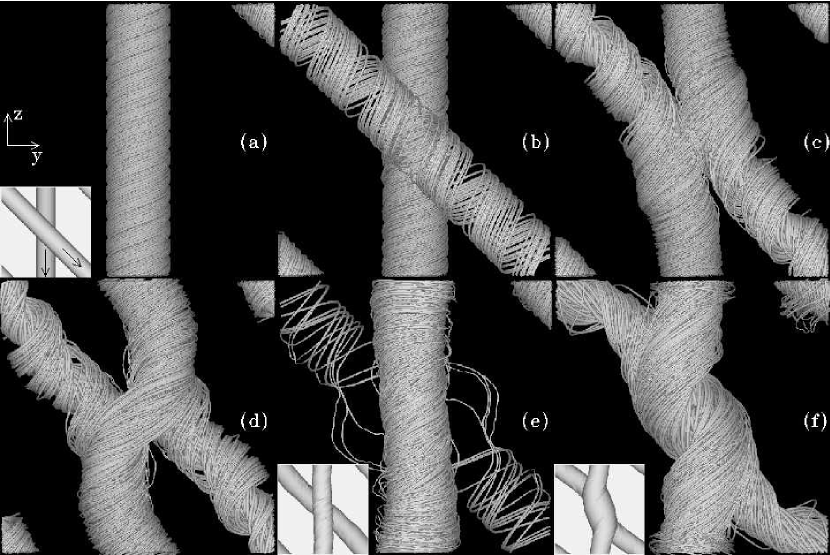
Figure 15: Fieldlines from simulation RR7 at ${\mathcal{T}}=4$ and for a nonuniform Lunquist numberwith a maximum of $57,600$. This simulation shows three separate reconnection interactions: the tubes first slingshot by panel (d), then tunnel by panel (e), and finally merge together by panel (f). The panels shown here are at times $tv_{A}/R=[0,7,25,40,78,202]$.

We will now study the effect that the flux tube collision angle has on the tunnel and slingshot reconnections. The analytical theory shows that the tunnel should occur for any pair of positively twisted tubes crossing at an angle $\pi<\theta<2\pi$. At collision angles of $N\pi/4$ this should include $N=5$, $6$, and $7$. The RR5 and RR7 interactions were studied by Linton et al., (2001) at a uniform $S_{\eta}=2880$, but a definitive tunnel was not seen in either case. The RR5 interaction bounced with little reconnection, while the RR7 interaction tunneled partway and then stopped, leaving the two tubes entangled (see Fig. 15 of Linton et al.,, 2001). As we can now perform these simulations at a higher Lundquist number, using the localized resistivity to keep the codes stable, we have revisited these simulations to see if the tunnel occurs when diffusive loss of twist plays less of a role.

For a simulation at a background Lundquist number of $288,000$ and a collision region Lundquist number of $2880$, we found that the RR5 tubes simply bounced at high twist, as they did in our original simulations for uniform a Lundquist number of $2880$. However, surprisingly, at a lower Lundquist number of $57,600$ globally and $576$ locally, we found that the RR5 flux tubes do tunnel. In this case, it appears that a $lower$ $L_{\eta}$ in the reconnection region is important, at least for a collision speed of $.025v_{A}$. Apparently at too high a Lundquist number, the tubes bounce before reconnection can take hold. This suggests that the tubes might reconnect at higher Lundquist numbers if the velocity of collision were lower.

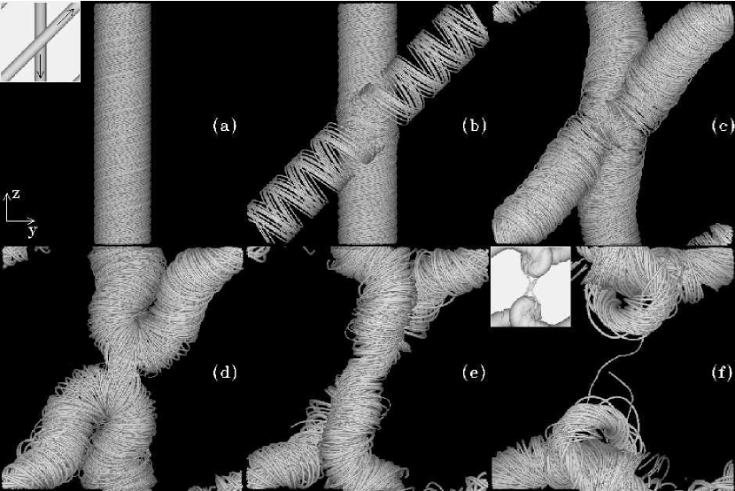
Figure 10: Fieldlines from simulation RR5 at ${\mathcal{T}}=7$ and for a nonuniform Lunquist number with a maximum of $57,600$. At this level of twist the tubes slingshot. The panels shown here are at times $tv_{A}/R=[0,7,32,81,125,248]$.

For these $L_{\eta}=57,600$ simulations, we found a transition from tunnel to slingshot at a twist of ${\mathcal{T}}=7.5$ to $7$. The ${\mathcal{T}}=7$ slingshot simulation is shown in Figure 10. Figure 10(a) shows the fieldlines of the vertical tube and, in the inset, isosurfaces of both tubes with arrows indicating the directions of the axial fields. The field reconnects from Figures 10(b) through 10(d) to form two $U$ shaped flux tubes which are ready to slingshot away from each other to the top and bottom of the simulation. But, as there is almost enough twist here for the tubes to tunnel, a number of fieldlines tunnel before the tubes slingshot. These fieldlines briefly dominate the interaction so that the field in Figure 10(e) looks like it has almost tunneled. However, this attempt does not succeed, the tunneled fieldlines are pulled back, and the tubes slingshot into highly kinked flux tubes by Figure 10(f). This final slingshot state contrasts with the ${\mathcal{T}}=1$ RR6 slingshot of Figure 1, where the tubes do not kink at all. The difference is that the tubes here are highly twisted. While the initial state is only slightly kink unstable, the slingshot shortens the tubes significantly, concentrating their twist, and making them much more kink unstable. When the tubes kink, this stretches them to the optimal length at which the sum of axial and twist field energy is at a minimum (see Linton et al.,, 1999).

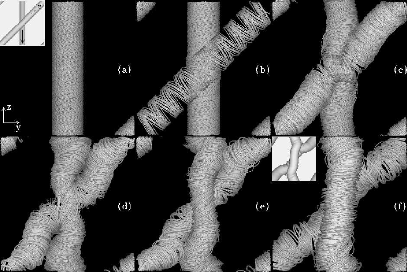
Figure 11: Fieldlines from simulation RR5 at ${\mathcal{T}}=7.5$ and for a nonuniform Lunquist number with a maximum of $57,600$. At this level of twist the tubes tunnel. The panels shown here are at times $tv_{A}/R=[0,7,32,79,106,261]$.

The ${\mathcal{T}}=7.5$ tunnel simulation is shown for comparison in Figure 11. As for the RR6 simulation, the early part of this reconnection, in Figures 11(b) through 11(d) looks very much like the corresponding slingshot reconnection at lower twist in Figures 10(b) through 10(d). But again, there are more tunneled fieldlines by Figure 11(e) than there are for the slingshot in Figure 10(e). In this case, these fieldines are strong enough to dominate the interaction, and so by Figure 11(f) the flux tubes have largely tunneled. This is not as clean a tunnel as for the RR6 interaction, as is shown by the fact that a number of the diagonal fieldlines have not become disconnected from the vertical flux tube and disappeared, but still a large part of the flux has tunneled. Comparing the isosurfaces inset into Figure 11(a) and 11(f) gives further evidence of tunneling by showing that the tubes have switched positions. The isosurfaces also show that there is significantly more diffusion in this simulation than in the RR6 simulation at $5$ times the Lundquist number. The isosurfaces of the RR6 tunneled flux tubes in Figure 7(f) are not discernibly thicker than they were initially in 7(f). But the isosurfaces of the RR5 tunneled flux tubes in Figure 11(f) are $30\%$ to $50\%$ thicker than they were initially, in Figure 11(f), indicating that the tubes have spread out radially due to diffusion.

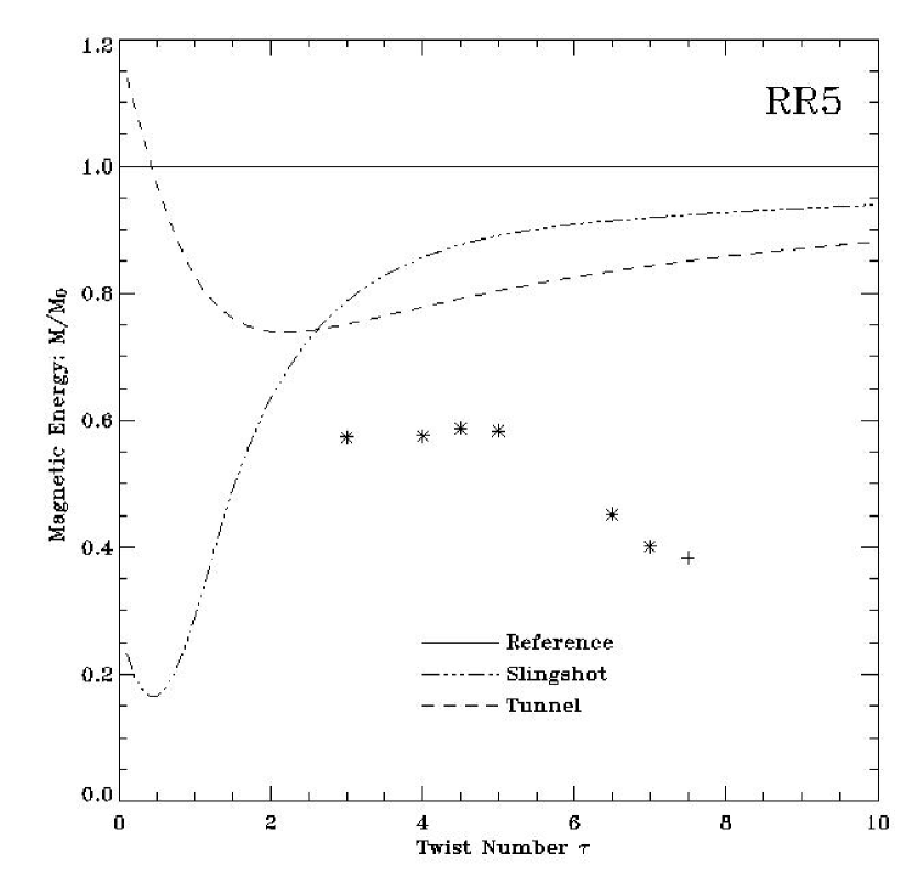
Figure 12: Theoretical reconnection energy, as in Figure 5, for RR5 simulations. The asterisks denote simulation values for slingshot interactions, while the plus sign denotes the simulation value for the tunnel interaction of Figure 11.

The energy prediction for RR5 reconnections as a function of twist is shown in Figure 12. This looks quite similar to that for RR6 interactions, and level of twist below which the slingshot is predicted to lose more energy than the tunnel is about the same, at ${\mathcal{T}}=2.62$. Thus, while the tunnel does occur at $\theta=5\pi/4$ as predicted, the transition from tunnel to slingshot, at ${\mathcal{T}}=7.5$ to $7$, occurs at a twist almost three times larger than predicted by energy release alone, at least for this level of resistivity. This large discrepancy could be partly due to the lower value of Lundquist number used here: a third of the helicity is lost to diffusion in the ${\mathcal{T}}=7.5$ RR5 simulation, and so we expect an equivalent percentage of the twist was also lost to diffusion. But the second, and likely more important effect, is that it is very difficult for the slingshot flux tubes to reconnect again once they have lost contact. As can be seen from Figure 10(f), the slingshot tubes end up very far from each other. While their optimal length is fairly long due to their high twist, they do not settle into $U$ shaped loops of this length, which might keep them in contact, but rather settle into kinked loops of this length. Thus, as in the RR6 simulations, the tunnel may be a lower energy state at twists well below ${\mathcal{T}}=7$, but it is simply inaccessible to the tubes, and so does not occur. For comparison, the estimated energy release of the various slingshot and tunnel interactions we simulated are plotted on Figure 12. These measured values of energy release do not agree as well with the predicted values as they do in the RR6 reconnection, but given the relatively high level of resistivity we had to use for these simulations, and the long time it took for the interaction to finish, this is only to be expected. There is also evidence that these tubes evolve significantly towards a lower energy constant $\alpha$ Taylor state: the initial standard deviation of $\alpha$ is $2.6$ relative to a standard deviation of $1.5$ after the tunnel.

7 RR7 Reconnection

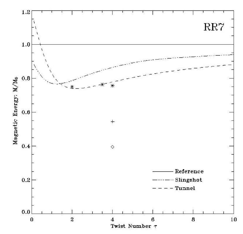
Figure 13: Theoretical reconnection energy, as in Figure 5, for RR7 simulations. The asterisks denote simulation values for slingshot interactions, while the plus sign denotes the simulation value for the tunnel interaction of Figure 15(e), and the diamond denotes the simulation value for the merge interaction of Figure 15(f).

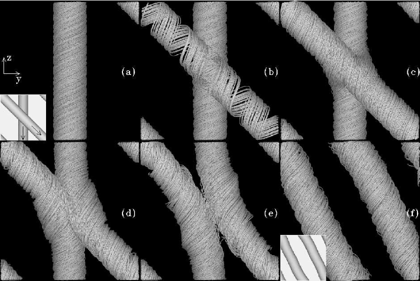
Figure 14: Fieldlines from simulation RR7 at ${\mathcal{T}}=3.5$ and for a nonuniform Lunquist number with a maximum of $57,600$. At this level of twist the tubes slingshot. The panels shown here are at times $tv_{A}/R=[0,7,13,19,25,190]$.

For our final set of simulations, we investigated the reconnection of RR7 flux tubes. Here, we found that the code was more unstable than for the RR6 collisions, so we had to decrease the nonuniform Lundquist number by a factor of $5$ to $57,600$ globally, and $576$ locally, as for the RR5 simulations. At this level of resistivity we found that there is indeed a clear tunnel interaction, and that the transition from tunnel to slingshot occurs at a twist of ${\mathcal{T}}=4$ to $3.5$, respectively. The energy prediction for this interaction, shown in Figure 13, indicates that the slingshot becomes preferable below twists of about $1.41$, so again the actual level at which the transition occurs is a factor of two to three higher than the energy analysis predicts. Figure 14 shows the ${\mathcal{T}}=3.5$ slingshot interaction. This interaction is quite straightforward, but also quite interesting in that the angle, $7\pi/4=-\pi/4$, between the axial field of the flux tubes is so small. Even at this small angle, the flux tubes reconnect completely because of the coherence that the twist induces. The flux tubes reconnect from Figures 14(b) through 14(e) to form a simple pair of cylindrical, twisted flux tubes by the end of the simulation in Figure 14(f).

In contrast, the tunnel reconnection at ${\mathcal{T}}=4$, shown in Figure 15 is quite an involved interaction. The tubes start off by reconnecting to slingshot in Figures 15(b) and 15(c). But they do not completely separate: some of the flux has already tunneled by the time the tubes try to slingshot away from each other, and this keeps them together. The tubes then reconnect a second time in Figure 15(d) to tunnel by Figure 15(e). Only a few diagonal fieldlines are still connected to the vertical tube at this time, and so these fieldlines are mostly invisible. The isosurface inset in Figure 15(e) presents further evidence of the tunnel when compared with the initial isosurface in Figure 15(a). But the reconnection does not stop here. By tunnelling, the tubes move from an RR7 configuration to an RR1 configuration. This can be seen by rotating the simulation about the ${\bf\hat{z}}$ axis so that the vertical flux tube is behind the horizontal flux tube, as per our convention: in this orientation, the tubes cross each other at $\theta=\pi/4$. But this is the configuration for which Linton et al., (2001) found that the azimuthal component of the field reconnects to merge the two tubes into a single tube (see Fig. 8 of Linton et al.,, 2001). Exactly the same thing happens here: the newly tunneled RR1 flux tubes merge together to form a single flux tube at the center of the simulation, while the boundary conditions keep the footpoints well separated. This RR7 simulation therefore exhibits three full flux tube reconnections: a slingshot, followed by a tunnel, and then by a merge. It is now apparent that we saw approximately the same thing in our RR7, $S_{\eta}=2880$ simulations in Linton et al., (2001): due to the faster rate of overall diffusion there, the tubes started to merge before completing the tunnel, and so the simulation looked like a failed tunnel interaction.

Magnetic energy is released by reconnection at each of these three stages. The estimated measurements of this energy release are shown on Figure 13, where the asterisks and the plus sign are the slingshot and tunnel energies, respectively, and the diamond is the energy of the merged end state. The results for the slingshot at ${\mathcal{T}}=3.5$ and a second slingshot at ${\mathcal{T}}=2$ are also shown. These energy results are reasonably close to the predicted values for the slingshot, probably because the slingshot occurs very quickly, and so there is little time for diffusive losses. Interestingly, in this case the standard deviation of $\alpha$ is $1.6$ after tunneling versus $1.5$ initially, so the tubes do not appear to have evolved to a constant $\alpha$ state. Once the tubes merge, however, the standard deviaton of $\alpha$ has dropped to $1.1$. These three tunnel results in combination provide a convincing argument for revisiting the energy calculation of Linton & Antiochos, (2002) to calculate the final energy state for flux tubes which evolve to constant $\alpha$ force free states.

8 Conclusion

We have studied tunneling reconnection for a variety of flux tube collision angles, flux tube twists, and resistive Lundquist numbers. We have compared the results with predictions made by the analytical theory of Linton & Antiochos, (2002). The prediction that positive twist flux tubes crossing at angles in the range $\pi<\theta<2\pi$ will tunnel for high twist was proved true by our simulations: we found tunneling interactions at collision angles of $5\pi/4$, $6\pi/4$, and $7\pi/4$. We also found that the tunnel transitions to slingshot as twist decreases, as predicted by the theory, but that the level of twist at which the transition occurs is two to three times higher than predicted. We hypothesize that this is due to the dynamics of the reconnection process, which were not included in the theory. When flux tubes reconnect the first time to slingshot, they spring away from each other and can come to a new equilibrium wherein they are not in contact with each other. If this occurs, the tubes cannot reconnect again to tunnel, even if the tunnel would allow them to reach a lower energy state than that of the slingshot state. The magnetic energy released by these interactions is reasonably well predicted by the theory, if allowances for diffusive losses are made. For simulations at very high Lundquist numbers, or simulations which progressed quickly and therefore allowed little time for energy to diffuse resistively, the predicted reconnection energy release is within a factor of two of the energy released in the simulation. As resistivity plays a larger role in the dynamics, however, more magnetic energy is lost to resistivity, independent of reconnection, and so there is a larger discrepancy between the simulation and the theory. In addition to resistive losses, we also find evidence that the tubes evolve towards constant $\alpha$ equilibria after reconnection, rather than constant twist as we have assumed: this would allow for further magnetic energy release.

For reconnection in the solar corona, where the Lundquist number is extremely high, diffusive losses should be negligible, and so the prediction for reconnection energy release should be in better agreement with the total energy release than it is in our modest Lundquist number simulations. The transition from tunnel to slingshot, however, is not expected to change significantly as the Lundquist number increases, and so we expect that the actual transition would still be $2$ to $3$ times higher than predicted. This means that only very highly twisted flux tubes are expected to tunnel, and so this should be relatively rare on the Sun. It should only occur for the small, highly twisted features observed within larger scale, less twisted sunspots (Canfield, private communication), and for those highly twisted convection zone flux tubes which are too twisted to successfully emerge into the corona, because too much mass is entrained in their highly twisted loops (Fan,, 2001; Magara & Longcope,, 2001). In addition to these solar applications, this study is important as a general study of the role that helicity conservation plays in reconnection. As we have shown here, it can have profound effects, and therefore needs to be taken into account when modeling three-dimensional reconnection. In addition, as the slingshot reconnection occurs down to zero twist, the theory of Linton & Antiochos, (2002) as it relates to slingshot energy release could prove useful for predicting energy release in solar interactions. To explore the true usefulness of these predictions, we need to modify the theory, first to study constant $\alpha$ final equilibria, and second to encompass arched magnetic flux tubes so that the simulations can better match solar conditions. We also need to increase the resolution of our simulations so that we can increase the Lundquist number without inducing numerical instability. We will then be able to test whether the agreement between the predicted energy release and the simulated release continues to improve as the diffusive losses decrease.

References

- Antiochos et al., (1999) Antiochos, S. K., DeVore, C. R., & Klimchuk, J. A. 1999, ApJ, 510, 485
- Berger, (1987) Berger, M. 1987, JGR, 102, 2637
- Berger & Field, (1984) Berger, M. & Field, G. 1984, JFM, 147, 133
- Dahlburg et al., (1997) Dahlburg, R. B., Antiochos, S. K., & Norton, D. 1997, Phys. Rev. E, 56, 2094
- Dahlburg & Norton, (1995) Dahlburg, R. B. & Norton, D. 1995, in Small Scale Structures in Three-Dimensional Hydrodynamic and Magnetohydrodynamic Turbulence, ed. M. Meneguzzi, A. Pouquet, & P. Sulem, (Heidelberg: Springer-Verlag), 317
- Fan, (2001) Fan, Y. 2001, ApJ, 554, L111
- Finn & Antonsen, (1985) Finn, J. M. & Antonsen, M. A. 1985, Comments Plasma Phys. Controlled Fusion, 9, 111
- Gold & Hoyle, (1960) Gold, T. & Hoyle, F. 1960, MNRAS, 120, 89
- Gosling, (1975) Gosling, J. T. 1975, Rev. Geophys. Space Phys., 13, 1053
- Hornig, (2005) Hornig, G. 2005, in preparation
- Linton & Antiochos, (2002) Linton, M. G. & Antiochos, S. K. 2002, ApJ, 581, 703
- Linton et al., (2001) Linton, M. G., Dahlburg, R. B., & Antiochos, S. K. 2001, ApJ, 553, 905
- Linton et al., (1998) Linton, M. G., Dahlburg, R. B., Longcope, D. W., & Fisher, G. H. 1998, ApJ, 507, 404
- Linton et al., (1999) Linton, M. G., Fisher, G. H., Dahlburg, R. B., & Fan, Y. 1999, ApJ, 522, 1190
- Linton & Priest, (2003) Linton, M. G. & Priest, E. R. 2003, ApJ, 595, 1259
- Magara & Longcope, (2001) Magara, T. & Longcope, D. W. 2001, ApJ, 559, L55
- Mikić & Linker, (1994) Mikić, Z. & Linker, J. A. 1994, ApJ, 430, 898
- Parker, (1972) Parker, E. N. 1972, ApJ, 174, 499
- Press et al., (1986) Press, W. H., Flannery, B. P., Teukolsky, S. A., & Vetterling, W. T. 1986, Numerical Recipes: The art of scientific computing, (Cambridge: Cambridge University Press)
- Priest et al., (2002) Priest, E. R., Heyvaerts, J. R., & Title, A. M. 2002, ApJ, 576, 533
- Rosner et al., (1978) Rosner, R., Tucker, W. H., & Vaiana, G. S. 1978, ApJ, 200, 643
- Schindler et al., (1988) Schindler, K., Hesse, M., & Birn, J. 1988, JGR, 93, 5547
- Schrijver, (1998) Schrijver, C. J. et al. 1998, Nature, 394, 152
- Shibata et al., (1995) Shibata, K., Masuda, S., Shimojo, M., Hara, H., Yokoyama, T., Tsuneta, S., Kosugi, T., & Ogawara, Y. 1995, ApJ, 451, L83
- Taylor, (1986) Taylor, J. 1986, Rev. Mod. Phys., 58, 741
- Wright & Berger, (1989) Wright, A. N. & Berger, M. A. 1989, JGR, 94, 1295