Hydrodynamic Turbulence in Accretion Disks

Abstract

Turbulent viscosity in cold accretion disks is likely to be hydrodynamic in origin. We investigate the growth of hydrodynamic perturbations in a small region of a disk, which we model as a linear shear flow with Coriolis force, between two parallel walls. Although there are no exponentially growing eigenmodes in this system, because of the non-normal nature of the modes, it is possible to have a large transient growth in the energy of certain perturbations. For a constant angular momentum disk, the energy grows by more than a factor of $1000$ for a Reynolds number of only $1000$, and so turbulence is easily excited. For a Keplerian disk, the growth is more modest, and energy growth by a factor of $1000$ requires a Reynolds number of nearly a million. Accretion disks have even larger Reynolds numbers than this. Therefore, transient growth of perturbations could seed turbulence in such disks.

I INTRODUCTION

The origin of hydrodynamic turbulence is still not completely understood. Many efforts have been devoted to solve this problem, beginning with the work of Kelvin, Rayleigh, and Reynolds at the end of the nineteenth century, to more recent work. In most cases, a significant mismatch has been found between the results based on linear theory and experimental (observational) data. In the laboratory, plane Poiseuille and plane Couette flows become turbulent at Reynolds numbers, $R\geq R^{\rm exp}_{c}\sim 1000$, $350$, respectively, while theoretically, plane Couette flow is linearly stable at all values of $R$ and plane Poiseuille is linearly unstable only for $R\geq R^{\rm the}_{c}=5772$. What is the reason for this mismatch? It would appear that for $R$ values in between $R=R^{exp}_{c}$ and $R=R^{the}_{c}$, some new effect allows the system to make a subcritical transition to turbulence in the absence of a linear instability.

In the field of astrophysics, hydrodynamics and turbulence find extensive applications. Accretion flows in binary stars, young stellar objects and active galactic nuclei must be turbulent in order for the gas to accrete. However the actual origin of the turbulence is unclear and still under debate. Inward mass accretion in a disk occurs as a result of the transfer of angular momentum outward by means of some viscous torque in the system. More than three decades ago, Shakura & Sunyaev ss and Lynden-Bell & Pringle lp proposed that turbulent viscosity provides the necessary viscous torque to cause inward mass transport. However, the physical origin of the turbulence in an accretion disk was unclear until the work of Balbus & Hawley bh who showed that magnetized disks have a Magneto-Rotational-Instability (MRI) veli ; chan in the presence of a weak magnetic field. This instability provides a natural means to generate turbulence and transport angular momentum outward. Later, Hawley, Gammie & Balbus hgb1 showed that the turbulence dies out if the Lorentz forces are turned off in a magnetohydrodynamically turbulent Keplerian disk. Subsequently they again showed hgb2 that the magnetic field dies out when the tidal and Coriolis forces are turned off, keeping the Lorentz forces. In two subsequent papers bhs ; hbw , it was shown through numerical simulations that, whereas pure hydrodynamic turbulence is easily triggered in plane Couette flow and in a constant angular momentum disk, turbulence does not develop in an unmagnetized Keplerian disk even in the presence of large initial perturbations. The authors argued on this basis that hydrodynamic turbulence cannot contribute to viscosity in accretion disks.

Despite the above results, it is probably premature to rule out hydrodynamic turbulence in rotationally supported disks. Many astrophysical systems are known, e.g., star-forming disks, cataclysmic variables in quiescence, outer regions of AGN disks, etc., in which the gas is cold and neutral so that there is negligible coupling between the magnetic field and the gas (see e.g., bb ; gm ; ftb ). In these systems, the Magneto-Rotational-Instability (MRI) cannot play a role. How do these systems sustain mass transfer in the absence of the MRI? What drives their turbulence? It is possible that the turbulence is purely hydrodynamic in origin. Even in the absence of exponentially growing modes, plane Couette flow is known to exhibit a large transient growth in energy for certain initial conditions. Is this transient growth responsible for the subcritical turbulence that occurs in this flow, and could a similar phenomenon be responsible for generating hydrodynamic turbulence in cold accretion disks? Recent laboratory experiments on rotating Couette flow in the narrow gap limit with linearly stable rotational angular velocity profiles (similar to Keplerian disks) seem to indicate that turbulence does manage to develop in such flows rz . Longaretti long points out that the absence of turbulence in the simulations bhs ; hbw may be because of their small effective Reynolds number.

Transient growth occurs in a linear system because of the non-normal nature of the associated operator bf ; rh ; tt . How, and if, such growth might finally cause turbulence is not well understood. One possibility is that the growth causes fluctuations to acquire large amplitudes, and non-linear interactions then push the system into self-sustained chaotic turbulence.

We present here some results on shearing rotating flows following the methods that have been developed to study the evolution of non-normal modes in plane Couette flow. We employ a local approximation, and focus mainly on an eigenvalue analysis of perturbations in Eulerian coordinates (for details, see man , and also amn ; bgam for a similar analysis in Lagrangian coordinates). In the next section, we briefly describe the basic model and write down the set of equations to be solved. Then in §3, we present a few important results. We conclude with a discussion in §4.

II MODEL

We consider a small patch of an accretion disk whose local geometry is described in terms of Cartesian coordinates, $x=(r-r_{0})$, $y=r_{0}(\phi-\phi_{0})$. We assume that the flow is incompressible and extends from $x=-1$ to $+1$, between two rigid walls with no-slip boundary conditions. The $y$ and $z$ directions are unbounded with periodic boundary conditions. This flow behaves like rotating Couette flow in the narrow gap limit, when the unperturbed velocity corresponds to a linear shear, $\vec{U}=(0,-x,0)$, and the Coriolis force is described by the angular frequency $\vec{\omega}=(0,0,1/q)$: $\Omega=\Omega_{0}(r_{0}/r)^{q}$. Here all the coordinates and quantities are expressed in terms of dimensionless variables. Note, $q=3/2$ corresponds to a Keplerian disk, $q=1$ and $2$ to a flat rotation curve and a constant angular momentum disk, respectively, and $q=0$ corresponds to rigid body rotation. A schematic diagram of the flow in the local coordinates is shown in Fig. 1.

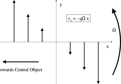
Figure 1: Unperturbed flow in the local shearing box. The arrows represent the velocity field.

Writing the perturbations as $U_{x}(x,y,z,t)\rightarrow u(x,y,z,t)$, $U_{y}(x,y,z,t)\rightarrow U_{y}(x)+v(x,y,z,t)$, $U_{z}(x,y,z,t)\rightarrow w(x,y,z,t)$, $P/\rho\rightarrow P/\rho+p(x,y,z,t)$, and combining the linearized Navier-Stokes and continuity equations, we obtain

$$\hskip-28.45274pt\left(\frac{\partial}{\partial t}+U\frac{\partial}{\partial y}\right)\nabla^{2}u-\frac{\partial^{2}U}{\partial x^{2}}\frac{\partial u}{\partial y}+\frac{2}{q}\frac{\partial\zeta}{\partial z}=\frac{1}{R}\nabla^{4}u,$$ (1)

$$\hskip-28.45274pt\left(\frac{\partial}{\partial t}+U\frac{\partial}{\partial y}\right)\zeta-\frac{\partial U}{\partial x}\frac{\partial u}{\partial z}-\frac{2}{q}\frac{\partial u}{\partial z}=\frac{1}{R}\nabla^{2}\zeta,$$ (2)

where $\zeta={\partial w}/{\partial y}-{\partial v}/{\partial z}$. Equations (1) and (2) are the standard Orr-Sommerfeld and Squire equations, respectively, except that they now have additional terms due to the presence of rotation in the system. We have to solve equations (1) and (2) with the boundary conditions: $u=\partial u/\partial x=\zeta=0$, at $x=\pm 1$ (no slip).

Due to translational invariance in the $y$ and $z$ directions, the perturbations can be chosen as $u(x,y,z,t)=\hat{u}(x)e^{i\sigma t}e^{i(k_{y}y+k_{z}z)}$ and $\zeta(x,y,z,t)=\hat{\zeta}(x)e^{i\sigma t}e^{i(k_{y}y+k_{z}z)}$, where $\sigma=\sigma_{R}+i\sigma_{I}$ is an eigenvalue of the problem. After substituting these perturbations in (1) and (2), we solve the combined Orr-Sommerfeld and Squire equations to obtain the eigensystem $\{\sigma,\hat{u},\hat{\zeta}\}$. The detailed set of equations and its reduction to an eigenvalue equation form and the solution procedure are described in man .

As mentioned above, even in the absence of any exponentially growing mode in the system, plane Couette flow can exhibit a large transient growth in the energy of certain perturbations bf ; tt . This growth occurs in the absence of non-linear effects and is believed to facilitate the transition from laminar to turbulent flow. The maximum growth in the perturbed energy can be expressed as

$$G_{K}(t)={\rm optimum}\left(\frac{E_{t}}{E_{0}}\right),$$ (3)

where

$$E_{t}=\frac{1}{8k^{2}}\int_{-1}^{1}\left[k^{2}\hat{u}^{\dagger}\hat{u}+\frac{\partial\hat{u}}{\partial x}^{\dagger}\frac{\partial\hat{u}}{\partial x}+\hat{\zeta}^{\dagger}\hat{\zeta}\right]dx$$ (4)

and $E_{0}$ is the initial energy of the perturbation at time $t=0$. By “optimum” we mean that we consider all possible initial perturbations and choose that function that maximizes the growth of energy at time $t$. To understand the technical details of how to compute the growth, see man .

III RESULTS

The eigenvalue analysis shows that, for plane Couette flow and for a rotating flow with $q\leq 2$, there are no exponentially growing modes in the system, i.e., for no choice of the parameters is there an eigenvalue with $\sigma_{I}>0$. However, for plane Couette flow, previous workers (e.g. bf ; rh ) have shown that there is a large transient growth even for $R=1000$. The interesting point is that the maximum growth in energy for plane Couette flow and a constant angular momentum disk ($q=2$) are very similar. Figure 2 shows the contours of constant maximum growth ($G_{\rm max}$) and the time at which the growth is maximized ($t_{\rm max}$) for both plane Couette and $q=2$. Whereas for $q=2$, $G_{\rm max}$ occurs exactly on the $k_{z}$ axis, for plane Couette flow it is slightly off the axis. This is the only difference between the two cases.

Figure 2: Contours of (a) $G_{\rm max}$ for plane Couette flow, where dashed contours correspond to $10,30,...90$; solid to $150,200,...600$; dotted to $700,800,...1100$; dot-dashed to $1150,1160,...1200$; (b) $t_{\rm max}$ for plane Couette flow, where dot-dashed contours correspond to $20,25,...45$; solid to $50,55,...100$; dotted to $110,120,...180$; (c) $G_{\rm max}$ for $q=2$ flow, where contour labels are the same as in (a); (d) $t_{\rm max}$ for $q=2$ flow, where contour labels are the same as in (b). All calculations are for $R=1000$.

Table 1

Maximum Growth for Various $q$ and $R=1000$

$q$	$k_{y}$	$k_{z}$	$G_{\rm max}$	$t_{\rm max}$
$1.5$	$1.21$	$0$	$13.04$	$8.8$
$1.7$	$1.06$	$0.74$	$13.4$	$9$
$1.9$	$0.54$	$1.44$	$23.75$	$12.4$
$1.99$	$0.04$	$1.8$	$122.8$	$27.3$
$2$	$0$	$1.66$	$1165.9$	$138.5$

Figure 3 shows how $G_{\rm max}$ and $t_{\rm max}$ vary as a function of Reynolds number, $R$, for plane Couette flow and $q=2$ flow. We see that $G_{\rm max}$ scales as $R^{2}$ and $t_{\rm max}$ as $R$ in both cases, again highlighting the similarity of the two flows. The physical reason is that a constant angular momentum disk has zero epicyclic frequency. Thus, the effect of rotation is essentially cancelled out, making the basic structure of the system very similar to that of plane Couette flow.

Figure 3: Solid and dotted lines correspond to plane Couette and a $q=2$ disk respectively.

For a given $R$, when $q$ slightly deviates from $2$, growth immediately reduces dramatically due to the introduction of a small epicyclic frequency ($=\kappa=\sqrt{2(2-q)}\Omega$). This indicates the dominant effect that $\kappa$ has on the fluid dynamics. Table 1 and Fig. 4a show how $G_{\rm max}$ and $t_{\rm max}$ change as $q$ decreases below 2. It is interesting to note that, for a $q=2$ flow the growth is maximum for $k_{y}=0$, while for a Keplerian disk ($q=1.5$) the growth is maximum for $k_{z}=0$. Therefore, the location of $G_{\rm max}$ moves in the $k_{y}-k_{z}$ plane systematically from one axis to the other, as $q$ is varied. Thus, for a constant angular momentum disk, we need to include vertical structure in the perturbations to understand the energy growth, whereas for a Keplerian disk a 2-dimensional analysis is sufficient.

Even though the growth decreases dramatically as $q$ falls below 2, nevertheless, at a given $q$, if the Reynolds number $R$ increases to a large enough value, the growth can become significant. In Fig. 4b, we show how the peak value of growth increases with increasing $R$ for Keplerian disks. It is found that $G_{\rm max}$ scales as $R^{2/3}$ and $t_{\rm max}$ as $R^{1/3}$ for large $R$. Therefore, while the presence of a finite epicyclic frequency has a strong dynamical effect on growth, it does not rule out a large growth. One just needs much larger values of $R$. Cold astrophysical accretion disks can have $R$ as high as $10^{10}$ or more, so large growth should in principle be easily achieved in such disks. Also at smaller $k_{y}$, $G_{\rm max}$ scales as $k_{y}^{2/3}$, while at larger $k_{y}$, $G_{\rm max}$ decreases as $k_{y}^{-4/3}$. At large $t$, $t_{\rm max}$ scales as $k_{y}^{-2/3}$. For a detailed derivation of these scaling relations, see man .

Figure 4: Growth curves for (a) $q=1.5$ (solid), $1.7$ (dotted), $1.9$ (dashed), $1.99$ (dot-dashed); other parameters are given in Table 1. (b) Growth curves for $q=1.5$ when $\{R=4000,k_{y}=1.2\}$ (solid), $\{R=1000,k_{y}=1.21\}$ (dotted), $\{R=500,k_{y}=1.29\}$ (dashed); $k_{z}=0$.

Figure 5: Development of the perturbed $x$-component of the velocity $u(x,y)$ as a function of time for the optimal perturbation with the maximum growth of energy in a Keplerian flow with $R=1000$. The perturbation has $k_{y}=1.21$, $k_{z}=0$, $t_{\rm max}=8.8$. Panels show the perturbation at (a) $t=0$, (b) $t=t_{\rm max}/2=4.4$, (c) $t=t_{\rm max}=8.8$, (d) $t=3t_{\rm max}/2=13.2$. Solid and dotted contours correspond to positive and negative values of $u$ respectively.

For a Keplerian flow the maximum growth occurs for $k_{y}\sim 1.2$, $k_{z}=0$. Figure 5 shows the development with time of the perturbed velocity component $u(x,y)$ corresponding to $R=1000$. We show snapshots corresponding to four times: $t=0$, $t_{\rm max}/2$, $t_{\rm max}$, $3t_{\rm max}/2$. The perturbations are seen to resemble plane waves that are frozen in the shearing flow. The initial perturbation at $t=0$ is a leading wave with negative $x$-wavevector $k_{x}$ and with $|k_{x}|\gg k_{y}$. With time, the wavefronts are straightened out by the shear, until at $t=t_{\rm max}$, the wavefronts are almost radial and $k_{x}\sim 0$. Then, at yet later times, the wave becomes trailing and the energy also decreases. The perturbations are very similar to the growing perturbation described by other authors cg ; tv ; ur .

IV DISCUSSION

We find that significant transient growth of perturbations is possible in a shear flow with Coriolis force between walls (see also yk ). This system is an idealized local analog of an accretion disk. Although the system does not have any unstable eigenmodes, nevertheless, because of the non-normal nature of the eigenmodes a significant level of transient energy growth is possible for appropriate choice of initial conditions. If the maximum growth exceeds the threshold for inducing turbulence, it is plausible that this mechanism could drive the system to a turbulent state. Presumably, once the system becomes turbulent it can remain turbulent as a result of nonlinear interactions and feedback among the perturbations.

In this mechanism of turbulence, the maximum energy growth and the time needed for this growth are probably the main factors that control the transition to hydrodynamic turbulence. As mentioned in §1, for plane Couette flow $R_{c}^{exp}\sim 350$ and according to our analysis, for $R=350$, $G_{\rm max}=145$, and the corresponding $t_{\rm max}=42.3$. Since a $q=2$ disk is very similar to plane Couette flow, the critical Reynolds number for turbulence in this case is also likely to be $R_{c}\sim 350$. For this $R$, $G_{\rm max}=143.5$ and $t_{\rm max}=48.3$.

Based on the above idea, we make the plausible assumption that the threshold energy growth factor needed for transition to turbulence in a shear flow is $E_{c}\sim 145$. Applying this prescription to the optimal two-dimensional perturbations of a Keplerian disk (§§2,3), we estimate the critical Reynolds number for a Keplerian flow to be $R_{c}\sim 3.4\times 10^{4}$, i.e., a factor of 100 greater than in the case of plane Couette flow. The corresponding $t_{\rm max}=28.3$, which is comparable to that in plane Couette flow, and is not too large compared to the accretion time-scale of a geometrically thin disk.

Instead of taking $R_{c}\sim 350$, we might wish to be conservative and take $R_{c}\sim 1000$ for plane Couette flow and $q=2$ flow. In this case, $G_{\rm max}\sim 1200$ and $t_{\rm max}\sim 120-140$. Applying the requirement of $E_{c}\sim 1200$ to a Keplerian flow, we find $R_{c}\sim 10^{6}$ and $t_{\rm max}\sim 100$. Now the critical Reynolds number is a factor of $1000$ greater than in the case of plane Couette flow.

An interesting result is that epicyclic motions in a differentially-rotating disk kill the growth dramatically and as a result the critical Reynolds number $R_{c}$ becomes higher. This also changes the optimum wavevector $\{k_{y},k_{z}\}$ of the perturbations needed to produce energy growth. For a constant angular momentum disk ($q=2$) and plane Couette flow, it is seen that growth is maximized for $k_{y}\sim 0$. Even for a very small shift in the value of $q$ below 2, the location of maximum growth moves significantly in the $k_{y}-k_{z}$ plane away from the $k_{z}$ axis. With decreasing $q$, the epicyclic motions of the disk increase, and correspondingly the optimum value of $k_{y}$ for growth increases while the optimum $k_{z}$ decreases. For a Keplerian disk, the growth is maximum for $k_{z}=0$ (on the $k_{y}$ axis). To the best of our knowledge, this change in the location of the maximum growth in the $k_{y}-k_{z}$ plane has not been commented upon prior to this work.

In earlier numerical simulations bhs ; hbw , the above reduction of growth due to the effect of epicyclic motion in the disk was already noticed. However, those authors then proceeded to rule out the possibility of hydrodynamic turbulence in Keplerian disks. We do not agree with this conclusion. As we have shown, Keplerian disks can support large transient energy growth, only they need much larger Reynolds numbers to achieve the same energy growth as plane Couette flow or a $q=2$ flow. The numerical simulations probably had effective Reynolds numbers $\lesssim 10^{4}$ (because of numerical viscosity) which is below our most optimistic estimate of the critical Reynolds number for a Keplerian flow. Thus, we suspect the simulations simply did not have sufficient numerical resolution to permit the turbulence. The same point has been made by other authors long ; ur .

We conclude with an important caveat. While the demonstration of large energy growth is an important step, it does not prove that Keplerian disks will necessarily become hydrodynamically turbulent. Umurhan & Regev ur have shown via two-dimensional simulations that chaotic motions can persist for a time much longer than the time scale $t_{\rm max}$ needed for linear growth. However, they also note that their perturbations must ultimately decline to zero in the presence of viscosity. To overcome this limitation, it is necessary to invoke three-dimensional effects. Secondary instabilities of various kinds, such as the elliptical instability (e.g. ker ), are widely discussed as a possible route to self-sustained turbulence in linearly perturbed shear flows. It remains to be seen if these instabilities are present in perturbed flows such as those shown in Figure 5.

- (1) N. Shakura, & R. Sunyaev, A&A, 24, 337, 1973.
- (2) D. Lynden-Bell, & J. Pringle, MNRAS, 168, 603, 1974.
- (3) S. Balbus, & J. Hawley, ApJ, 376, 214, 1991.
- (4) E. Velikhov, J. Exp. Theor. Phys. (USSR), 36, 1398, 1959.
- (5) S. Chandrasekhar, Proc. Natl. Acad. Sci., 46, 53, 1960.
- (6) J. Hawley, C. Gammie, & S. Balbus, ApJ, 440, 742, 1995.
- (7) J. Hawley, C. Gammie, & S. Balbus, ApJ, 464, 690, 1996.
- (8) S. Balbus, J. Hawley, & J. Stone, ApJ, 467, 76, 1996.
- (9) J. Hawley, S. Balbus, & W. Winters, ApJ, 518, 394, 1999.
- (10) O. Blaes, & S. Balbus, ApJ, 421, 163, 1994.
- (11) C. Gammie, & K. Menou, ApJ, 492, L75, 1998.
- (12) S. Fromang, C. Terquem, & S. Balbus, MNRAS, 329, 18, 2002.
- (13) D. Richard, & J.-P. Zahn, A&A, 347, 734, 1999.
- (14) P. Longaretti, ApJ, 576, 587, 2002.
- (15) K. Butler, & B. Farrell, Phys. Fluids A, 4(8), 1637, 1992.
- (16) S. Reddy, & D. Henningson, J. Fluids Mech., 252, 209, 1993.
- (17) L. Trefethen, A. Trefethen, S. Reddy, & T. Driscoll, Science, 261, 578, 1993.
- (18) B. Mukhopadhyay, N. Afshordi, & R. Narayan, ApJ, submitted, 2004; astro-ph/0412193.
- (19) N. Afshordi, B. Mukhopadhyay, & R. Narayan, ApJ, submitted, 2004; astro-ph/0412194.
- (20) B. Johnson, & C. Gammie, ApJ, submitted, 2005; astro-ph/0501005.
- (21) G. Chagelishvili, J.-P. Zahn, A. Tevzadze, & J. Lominadze, A&A, 402, 401, 2003.
- (22) A. Tevzadze, G. Chagelishvili, J.-P. Zahn, R. Chanishvili, & J. Lominadze, A&A, 407, 779, 2003.
- (23) O. Umurhan, & O. Regev, A&A, 427, 855, 2004.
- (24) P. Yecko, A&A, 425, 385, 2004.
- (25) R. Kerswell, Ann. Rev. Fluid Mech., 34, 83, 2002.