Can Gamma-Ray Bursts Be Used to Measure Cosmology?
A Further Analysis

Abstract

Three different methods of measuring cosmology with gamma-ray bursts (GRBs) have been proposed since a relation between the $\gamma$-ray energy $E_{\gamma}$ of a GRB jet and the peak energy $E_{p}$ of the $\nu F_{\nu}$ spectrum in the burst frame was reported by Ghirlanda and coauthors. In Method I, to calculate the probability for a favored cosmology, only the contribution of the $E_{\gamma}-E_{p}$ relation that is already best fitted for this cosmology is considered. We apply this method to a sample of 17 GRBs, and obtain the mass density $\Omega_{M}=0.15^{+0.45}_{-0.13}$ ($1\sigma$) for a flat $\Lambda$CDM universe. In Method II, to calculate the probability for some certain cosmology, contributions of all the possible $E_{\gamma}-E_{p}$ relations that are best fitted for their corresponding cosmologies are taken into account. With this method, we find a constraint on the mass density $0.14<\Omega_{M}<0.69$ ($1\sigma$) for a flat universe. In Method III, to obtain the probability for some cosmology, contributions of all the possible $E_{\gamma}-E_{p}$ relations associated with their unequal weights are considered. With this method, we obtain an inspiring constraint on the mass density $0.16<\Omega_{M}<0.45$ ($1\sigma$) for a flat universe, and a $\chi^{2}_{dof}=19.08/15=1.27$ for the concordance model of $\Omega_{M}=0.27$. Compared with the previous two methods, Method III makes the observed 17 GRBs place much more stringent confidence intervals at the same confidence levels. Furthermore, we perform a Monte Carlo simulation and use a larger sample to investigate the cosmographic capabilities of GRBs with different methods. We find that, a larger GRB sample could be used to effectively measure cosmology, no matter whether the $E_{\gamma}-E_{p}$ relation is calibrated by low-$z$ bursts or not. Ongoing observations on GRBs in the Swift era are expected to make the cosmological utility of GRBs progress from its babyhood into childhood.

1 Introduction

The traditional cosmology has been revolutionized by modern sophisticated observation techniques in distant Type Ia supernovae (SNe Ia) (e.g. Riess et al. 1998; Schmidt et al. 1998; Perlmutter et al. 1999), cosmic microwave background (CMB) fluctuations (e.g. Bennett et al. 2003; Spergel et al. 2003), and large-scale structure (LSS) (e.g. Allen et al. 2003; Tegmark et al. 2004). Each type of cosmological data trends to play an unique role in measuring cosmology. In modern cosmology, it has been convincingly suggested that the global mass-energy budget of the universe, and thus its dynamics, is dominated by a dark energy component, and that the currently accelerating universe has once been decelerating (e.g., Riess et al. 2004). The cosmography and the nature of dark energy as well as its evolution with redshift are one of the most important issues in physics and astronomy today.

Gamma-ray bursts (GRBs) are the most intense explosions observed so far. They are believed to be detectable up to a very high redshift (Lamb & Reichart 2000; Ciardi & Loeb 2000; Bromm & Loeb 2002; Gou et al. 2004), and their high energy photons are almost immune to dust extinction. These advantages would make GRBs an attractive cosmic probe.

From the isotropic-equivalent peak luminosity $L_{\rm iso}-$variability (or spectral lag) relation (Fenimore & Ramirez-Ruiz 2000; Norris, Marani, & Bonnell 2000), the standard energy reservior $E_{\gamma}$ of GRB jets (Frail et al. 2001), the $L_{\rm iso}-$ peak energy $E_{p}$ of the $\nu F_{\nu}$ spectrum in the burst frame relation (Lloyd-Ronning & Petrosian 2002; Lloyd-Ronning & Ramirez-Ruiz 2002; Yonetoku et al. 2004), the isotropic-equivalent energy $E_{\rm iso}-E_{p}$ relation (Amati et al. 2002) to the beaming-corrected energy $E_{\gamma}-E_{p}$ relation (Ghirlanda et al. 2004a, Ghirlanda relation hereafter), GRBs are towards more and more standardizable candles. However, these relations in GRBs have not been calibrated by a low-$z$ GRB sample, so one should look for a method which is different from the “Classical Hubble Diagram” method in SNe Ia.

The luminosity relations with the variability and spectral lag make GRBs a distance indicator in the same sense as Cepheids and SNe Ia, in which an observed light-curve property can yield an apparent distance modulus (DM). Schaefer (2003) considered these two relations for nine bursts with known redshifts and advocated a new cosmographic method (hereafter Method I) for GRBs. In Method I, one first calibrates the two relations with the observed sample for a certain cosmology, and then applies the best-fit relations back to the observed sample to obtain a $\chi^{2}$ or a probability $P\propto{\rm exp(-\chi^{2}/2)}$ for this cosmology. Similar to the brightness of SNe Ia, the energy reserviors in GRB jets are also clustered, but they are not fine enough for precise cosmology (Bloom et al. 2003). Amati et al. (2002) found $E_{\rm iso}\propto{E_{p}}^{k}$ ($k\sim 2$) relation from 12 BeppoSAX bursts. The HETE-2 observations confirm this relation and extend it to X-ray flashes (Sakamoto et al. 2004a; Lamb et al. 2004). In addition, it also holds within a GRB (Liang, Dai & Wu 2004). The Ghirlanda relation is written as $(E_{\gamma}/10^{50}{\rm ergs})=C({E_{p}/100\rm keV})^{a}$, where $a$ and $C$ are dimensionless parameters. Theoretical explanations of this relation include the standard synchrotron mechanism in relativistic shocks (Zhang & Mészáros 2002; Dai & Lu 2002) together with the afterglow jet model, or the emission from off-axis relativistic jets (Yamazaki, Ioka & Nakamura 2004; Eichler & Levinson 2004; Levinson & Eichler 2005). This relation could also be understood due to comptonization of the thermal radiation flux that is advected from the base of an outflow in the dissipative photosphere model (e.g. Rees & Mészáros 2005). If these explanations are true, the Ghirlanda relation appears to be intrinsic. Thus, Dai, Liang & Xu (2004; DLX04) considered the Ghirlanda relation for 12 bursts and proposed another cosmographic method (hereafter Method II) for GRBs. In Method II, one makes marginalizations over the unknown parameters in the Ghirlanda relation to obtain a $\chi^{2}$ or a probability $P\propto{\rm exp(-\chi^{2}/2)}$ for a certain cosmology. Following Schaefer’s method, Ghirlanda et al. (2004b; GGLF04) and Friedman & Bloom (2004; FB04) also investigated the same issue but used different GRB data. Recently, Firmani et al. (2005; FGGA05) considered the Ghirlanda relation for 15 bursts and proposed a Bayesian approach for the cosmological use (hereafter Method III). In Method III, to obtain the probability for a certain cosmology, one considers contributions of all the possible $E_{\gamma}-E_{p}$ relations associated with their unequal weights. The detailed procedures of the three methods are shown in $\S 2.1$, which indicate that Method III is the optimized one.

As analyzed previously, due to the lack of low-$z$ GRBs, Methods I, II and III are different from the “Classic Hubble Diagram” method in SNe Ia. In this paper, we investigate the constraints on cosmological parameters from the observed 17 GRBs with different methods. Because the present GRB sample is a small one, it is necessary to use a large simulated sample, which may be established in the Swift era, to discuss the cosmographic capabilities with different methods.

This paper is arranged as follows. In $\S 2$, we describe our analytical methods and data. The results from the observed GRB sample are presented in $\S 3$. In $\S 4$, we perform Monte Carlo simulations and analyze the results from the simulated GRB sample. Conclusions and discussion are presented in $\S 5$.

2 Method and Sample Analysis

2.1 Method Analysis

According to the relativistic fireball model, the emission from a spherically expanding shell and from a jet is similar to each other, if the observer is along the jet’s axis and the Lorentz factor of the fireball is larger than the inverse of the jet’s half-opening angle $\theta$; but when the Lorentz factor drops below $\theta^{-1}$, the jet’s afterglow light curve is expected to present a break because of the edge effect and the laterally spreading effect (Rhoads 1999; Sari, Piran & Halpern 1999). Therefore, together with the assumptions of the initial fireball emitting a constant fraction $\eta_{\gamma}$ of its kinetic energy into the prompt $\gamma$-rays and a constant circumburst particle density $n$, the jet’s half-opening angle is derived to be

$$\theta=0.163\left({\frac{{t_{j,d}}}{{1+z}}}\right)^{3/8}\left({\frac{{n_{0}}}{{E_{{\rm iso},52}}}\frac{{\eta_{\gamma}}}{1-\eta_{\gamma}}}\right)^{1/8},$$ (1)

where $E_{{\rm iso},52}=E_{{\rm iso}}/10^{52}{\rm ergs}$, $t_{{\rm j},d}=t_{\rm j}/1\,{\rm day}$, $n_{0}=n/1\,{\rm cm}^{-3}$. The “bolometric” isotropic-equivalent $\gamma$-ray energy of a GRB is given by

$$E_{{\rm iso}}=\frac{4\pi d_{L}^{2}S_{\gamma}k}{1+z},$$ (2)

where $S_{\gamma}$ is the fluence (in units of erg cm^-2) received in an observed bandpass and the quantity $k$ is a multiplicative correction of order unity relating the observed bandpass to a standard rest-frame bandpass (1-$10^{4}$ keV in this paper) (Bloom, Frail & Sari 2001). The energy release of a GRB jet is thus given by

$$E_{\gamma}=(1-\cos\theta)E_{\rm iso},$$ (3)

with the fractional uncertainty (FB04) being

$$\left({\frac{{\sigma_{E_{\gamma}}}}{{E_{\gamma}}}}\right)^{2} = (1-\sqrt{C_{\theta}})^{2}\left[{\left({\frac{{\sigma_{S_{\gamma}}}}{{S_{\gamma}}}}\right)^{2}+\left({\frac{{\sigma_{k}}}{k}}\right)^{2}}\right]+C_{\theta}$$ (4)

$$\times\left[{\left({\frac{{3\sigma_{t_{j}}}}{{t_{j}}}}\right)^{2}+\left({\frac{{\sigma_{n_{0}}}}{{n_{0}}}}\right)^{2}+\left({\frac{{\sigma_{\eta_{\gamma}}}}{{\eta_{\gamma}-\eta^{2}_{\gamma}}}}\right)^{2}}\right],$$

where

$$C_{\theta}=\left[{\theta\sin\theta/(8-8\cos\theta)}\right]^{2}.$$ (5)

The Ghirlanda relation is

$$(E_{\gamma}/10^{50}{\rm ergs})=C(E_{p}/100\,{\rm keV})^{a},$$ (6)

where $a$ and $C$ are assumed to have no covariance, and $E_{p}=E^{obs}_{p}(1+z)$. Combining Eqs. (1), (2), (3) and (6), we derive the apparent luminosity distance with the small angle approximation (i.e., $\theta\ll 1$) as

$$d_{L}=7.575\frac{{(1+z)C^{2/3}[E_{p}^{obs}(1+z)/100\,{\rm keV}]^{2a/3}}}{{(kS_{\gamma}t_{j,d})^{1/2}(n_{0}\eta_{\gamma})^{1/6}}}{\rm{Mpc}},$$ (7)

Assuming that all the observables are independent of each other and their errors satisfy Gaussian distributions, we derive the fractional uncertainty of the apparent luminosity distance without the small angle approximation,

$$\left({\frac{{\sigma_{d_{L}}}}{{d_{L}}}}\right)^{2} = \frac{1}{4}\left[{\left({\frac{{\sigma_{S_{\gamma}}}}{{S_{\gamma}}}}\right)^{2}+\left({\frac{{\sigma_{k}}}{k}}\right)^{2}}\right]+\frac{1}{4}\frac{{1}}{{(1-\sqrt{C_{\theta}})^{2}}}\left[\left({\frac{{\sigma_{C}}}{C}}\right)^{2}\right.$$ (8)

$$\left.+\left({a\frac{{\sigma_{E_{p}^{obs}}}}{{E_{p}^{obs}}}}\right)^{2}+\left({a\frac{{\sigma_{a}}}{a}\ln\frac{E_{p}}{100}}\right)^{2}\right]+\frac{1}{4}\frac{C_{\theta}}{{(1-\sqrt{C_{\theta}})^{2}}}$$

$$\times\left[{\left({\frac{{3\sigma_{t_{j}}}}{{t_{j}}}}\right)^{2}+\left({\frac{{\sigma_{n_{0}}}}{{n_{0}}}}\right)^{2}}+\left({\frac{{\sigma_{\eta_{\gamma}}}}{{\eta_{\gamma}(1-\eta_{\gamma})}}}\right)^{2}\right].$$

For simplicity, we consider $\eta_{\gamma}=0.2$ and $\sigma_{\eta_{\gamma}}=0$ throughout this paper (Frail et al. 2001). The apparent DM of a burst can be given by

$$\mu_{\rm obs}=5\log d_{L}+25,$$ (9)

with the uncertainty of

$$\sigma_{\mu_{{\rm obs}}}=\frac{5}{\ln 10}\frac{\sigma_{d_{L}}}{d_{L}}.$$ (10)

On the other hand, the theoretical luminosity distance in $\Lambda$-models (Carroll, Press & Turner 1992) is given by

$$d_{L} = c(1+z)H_{0}^{-1}|\Omega_{k}|^{-1/2}{\rm sinn}\{|\Omega_{k}|^{1/2}$$ (11)

$$\times\int_{0}^{z}dz[(1+z)^{2}(1+\Omega_{M}z)-z(2+z)\Omega_{\Lambda}]^{-1/2}\},$$

where $\Omega_{k}=1-\Omega_{M}-\Omega_{\Lambda}$, and “sinn” is $\sinh$ for $\Omega_{k}>0$ and $\sin$ for $\Omega_{k}<0$. For $\Omega_{k}=0$, equation (11) degenerates to be $c(1+z)H_{0}^{-1}$ times the integral.

Usually, the likelihood for the parameters $\Omega_{M}$ and $\Omega_{\Lambda}$ can be determined from a $\chi^{2}$ statistic, where

$$\chi^{2}(\Omega_{M},\Omega_{\Lambda},a,C|h)=\sum\limits_{k}{\left[{\frac{{\mu_{{\rm{th}}}(z_{k};\Omega_{M},\Omega_{\Lambda}|h)-\mu_{{\rm{obs}}}(z_{k};\Omega_{M},\Omega_{\Lambda},a,C|h)}}{{\sigma_{\mu_{{\rm{obs}}}(z_{k};\,\Omega_{M},\,\Omega_{\Lambda},\,a,\,C,\,\sigma_{a}/a,\,\sigma_{C}/C)}}}}\right]}^{2},$$ (12)

where the dimensionless Hubble constant $h\equiv H_{0}/100\,\,{\rm{km\,s^{-1}Mpc^{-1}}}$ is taken as 0.71. If the Ghirlanda relation could be calibrated by low-$z$ bursts, the above $\chi^{2}$ statistic becomes the same as that in SNe Ia, that is,

$$\chi^{2}(\Omega_{M},\Omega_{\Lambda},h)=\sum\limits_{k}{\left[{\frac{{\mu_{{\rm{th}}}(z_{k};\Omega_{M},\Omega_{\Lambda},h)-\mu_{{\rm{obs,}}k}}}{{\sigma_{\mu_{{\rm{obs,}}k}}}}}\right]}^{2},$$ (13)

where $h$ should be marginalized.

The procedures of Method I , II and III are as follows:

Method I (see S03, GGLF04, FB04)

The procedure of this method is to (1) fix $\Omega_{i}\equiv(\Omega_{M},\Omega_{\Lambda})_{i}$, (2) calculate $\mu_{\rm th}$ and $E_{\gamma}$ for each burst for that cosmology, (3) best fit the $E_{\gamma}-E_{p}$ relation to yield $(a,C)_{i}$ and $(\sigma_{a}/a,\ \sigma_{C}/C)_{i}$, (4) substitute $(a,C)_{i}$ and $(\sigma_{a}/a,\ \sigma_{C}/C)_{i}$ into Eqs. (7) and (8), and thus derive $\mu_{\rm obs}$ and $\sigma_{\mu_{\rm obs}}$ for each burst for cosmology $\Omega_{i}$, (5) calculate $\chi^{2}$ for cosmology $\Omega_{i}$ by comparing $\mu_{\rm th}$ with $\mu_{\rm obs}$, $\sigma_{\mu_{\rm obs}}$, and then convert it to the probability by $P(\Omega_{i})\propto\exp(-\chi^{2}(\Omega_{i})/2)$ (Riess et al. 1998), (6) repeat Steps 1$-$5 from $i=1$ to $i={\rm N}$ to obtain the probability for each cosmology. Therefore, Method I is formulizd by

$$P(\Omega_{i})=P(\Omega_{i}|\Omega_{i})\,\,\,\,\,\,\,\,\,\,(i=1,\,{\rm N}).$$ (14)

Method II (see DLX04)

The procedure of this method is to (1) fix $\Omega_{i}$, (2) calculate $\mu_{\rm th}$ and $E_{\gamma}$ for each burst for that cosmology, (3) best fit the $E_{\gamma}-E_{p}$ relation to yield $(a,C)_{i}$ and $(\sigma_{a}/a,\ \sigma_{C}/C)_{i}$, (4) substitute $(a,C)_{i}$ and $(\sigma_{a}/a,\ \sigma_{C}/C)_{i}$ into Eqs. (7) and (8), and thus derive $\mu_{\rm obs}$ and $\sigma_{\mu_{\rm obs}}$ for each burst for cosmology $\Omega_{i}$, (5) repeat Steps 1$-$4 from $i=1$ to $i={\rm N}$ to obtain $\mu_{\rm th}$, $\mu_{\rm obs}$ and $\sigma_{\mu_{\rm obs}}$ for each burst for each cosmology;     (6) re-fix $\Omega_{j}$, (7) calculate $\chi^{2}(\Omega_{j}|\Omega_{i})$ by comparing $\mu_{\rm th}(\Omega_{j})$ with $\mu_{\rm obs}(\Omega_{i})$, $\sigma_{\mu_{\rm obs}}(\Omega_{i})$, and then convert it to a conditional probability by $P(\Omega_{j}|\Omega_{i})\propto\exp(-\chi^{2}(\Omega_{j}|\Omega_{i})/2)$, (8) repeat Step 7 from $i=1$ to $i=\rm N$ to obtain the probability for cosmology $\Omega_{j}$ by $P(\Omega_{j})\propto\sum\limits_{i}{\exp(-\chi^{2}(\Omega_{j}|\Omega_{i})/2)}$, (9) repeat Steps 6$-$8 from $j=1$ to $j=\rm N$ to obtain the probability for each cosmology. Method II is described by

$$P(\Omega_{j})=\sum\limits^{\rm N}_{i=1}{P(\Omega_{j}|\Omega_{i})}\,\,\,\,\,\,(j=1,\,{\rm N}).$$ (15)

Method III (see FGGA05)

Method III is an improvement of Method II. Its key idea is to consider unequal weights for different $E_{\gamma}-E_{p}$ relations, i.e., unequal weights for different conditional probabilities $P(\Omega_{j}|\Omega_{i})$. Therefore, the first seven steps of this method are the same as those of Method II. The follow-up procedure is to (8) repeat Step 7 from $i=1$ to $i=\rm N$ to obtain an iterative probability for cosmology $\Omega_{j}$ by $P^{\rm ite}(\Omega_{j})\propto\sum\limits_{i}{\exp(-\chi^{2}(\Omega_{j}|\Omega_{i})/2)\times P^{\rm ini}(\Omega_{i})}$ (here the initial probability $P^{\rm ini}(\Omega)$ for each cosmology is regarded as equal; e.g. $P^{\rm ini}(\Omega)\equiv 1$), (9) repeat Steps 6$-$8 from $j=1$ to $j=\rm N$ to obtain an iterative probability $P^{\rm ite}(\Omega)$ for each cosmology;     (10) replace $P^{\rm ini}(\Omega)$ on Step 8 with $P^{\rm ite}(\Omega)$ on Step 9, then repeat Steps 8$-$9, and thus reach another set of iterative probabilities for each cosmology, (11) run the above cycle again and again until probability for each cosmology converges, i.e. $P^{\rm ite}(\Omega)\Rightarrow P^{\rm fin}(\Omega)$ after tens of cycles.

In this method, to calculate the probability $P^{\rm fin}(\Omega_{j})$ for a favored cosmology, we consider contributions of all the possible $E_{\gamma}-E_{p}$ relations associated with their weights. The conditional probability $P(\Omega_{j}|\Omega_{i})$ denotes the contribution of some certain relation, and $P^{\rm fin}(\Omega_{i})$ weights the likelihood of this relation for its corresponding cosmology. Therefore, the Bayesian approach can be formulized by

$$P^{\rm fin}(\Omega_{j})=\sum\limits^{\rm N}_{i=1}{P(\Omega_{j}|\Omega_{i})\times P^{\rm fin}(\Omega_{i})}\,\,\,\,\,\,(j=1,{\rm N}).$$ (16)

However, FGGA05 took different calculations for the conditional probability $P(\Omega_{j}|\Omega_{i})$. Making use of the incomplete gamma function, they transformed $\chi^{2}(\Omega_{j}|\Omega_{i})$ into its corresponding conditional probability $P(\Omega_{j}|\Omega_{i})$. Actually, once the parameters $(a,C)_{i}$ and $(\sigma_{a}/a,\ \sigma_{C}/C)_{i}$ of the Ghirlanda relation are calibrated for cosmology $\Omega_{i}$, they become “known” for the cosmic model $\Omega_{j}$. So herein the meaning of $\chi^{2}(\Omega_{j}|\Omega_{i})$ is the same as that in SNe Ia. In this paper, we redefine the conditional probability $P(\Omega_{j}|\Omega_{i})$ by the formula of $P(\Omega_{j}|\Omega_{i})\propto\exp(-\chi^{2}(\Omega_{j}|\Omega_{i})/2)$.

2.2 Sample Analysis

The great diversity in GRB phenomena suggests that the GRB population may consist of substantially different subclasses (e.g. MacFadyen & Woosley 1999; Bloom et al. 2003; Sazonov et al. 2004; Soderberg et al. 2004). To make GRBs a standard candle, a homogenous GRB sample is required. The most prominent observational evidence for a GRB jet is its temporal break in their afterglow light curves. For some bursts, e.g., GRB030329, their temporal breaks are observed in both optical and radio bands. Berger et al. (2003) argued that these two breaks are caused by the narrow component and wide component of the jet in this burst, respectively, indicating that the physical origins of the breaks in the optical band and in the radio band are different. In addition, the radio afterglow light curves fluctuate significantly. For example, in the case of GRB970508, the light curve of its radio afterglow does not present clearly a break. Only a lower limit of $t_{j}>25$ days was proposed by Frail et al. (2000). Furthermore, the light curve of its optical afterglow is proportional to $t^{-1.1}$, in which case no break appears (Galama et al. 1998). We thus include only those bursts whose temporal breaks in optical afterglow light curves were well measured in our analysis. We obtain a sample of 17 GRBs excluding GRB970508. They are listed in Table 1.

We correct the observed fluence in a given bandpass to a “bolometric” bandpass of $1-10^{4}\ \rm{keV}$ with spectral parameters. The fluence and spectral parameters for a burst fitted by different authors may be affected by different criterions (or systematical biases) in their works. We thus collect a couple of fluence and spectral parameters from the same original literature. For GRB 970828, GRB 980703, GRB 991216, and GRB 011211, the fluence and spectral parameters are unavailable in the same original literature, so we choose their fluences measured in the widest energy band available in the other literature.

For GRB 011211, we approximately take the high-energy spectral index $\beta$ to be $-2.3$ because it is unreported in Amati (2004). The spectra of HETE-2-detected GRB020124, GRB020813, GRB021004, GRB030226 and XRF030429 are not fitted by the Band function but the cutoff power law model. However, it is appropriate that their corresponding “bolometric” fluences are calculated by the former model with $\beta\sim-2.3$, avoiding the potential systematical bias which is brought by applying different spectral models for one observed sample (Barraud et al. 2003).

The circumburst densities of several bursts in our sample have been obtained from broadband modelling of the afterglow emission (e.g., Panaitescu & Kumar 2002). For the bursts with unknown $n$, we assumed $n\simeq 3\,{\rm cm}^{-3}$ as the median value of the distribution of the measured densities, together with a constant fractional uncertainty of $80\%$ (Ghirlanda et al. 2004a; DLX04).

3 Cosmological Constraints

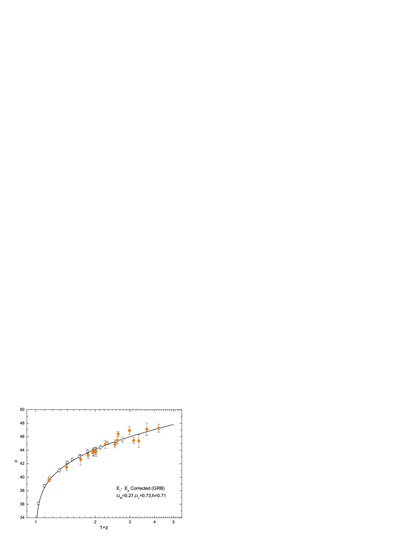
Figure 1: Hubble diagrams for the observed GRB sample (filled circles) and for the binned gold sample of SNe Ia (open circles). The GRB $E_{\gamma}-E_{p}$ relation has been calibrated in the cosmic model of $\Omega_{M}=0.27$, $\Omega_{\Lambda}=0.73$ and $h=0.71$ (solid line).

We first fit the $E_{\gamma}-E_{p}$ relation for the cosmology of $\Omega_{M}=0.27$, $\Omega_{\Lambda}=0.73$, and $h=0.71$, and obtain $a=1.53$, $C=0.97$, $\sigma_{a}/a=0.05$ and $\sigma_{C}/C=0.08$, together with the $\chi^{2}_{\nu}=21.93/15.0=1.46$, using Eq. (4) for the estimation of $\sigma_{E_{\gamma}}/E_{\gamma}$ (Press et al. 1999). Substituting the best-fit results into Eqs. (7) and (8), we plot the Hubble diagram for the observed GRB sample in the concordance model of $\Omega_{M}=0.27$, which is shown in Fig 1 (filled circles). Comparatively shown are the Hubble diagrams for the binned gold sample of SNe Ia (open circles; Riess et al. 2004), and the theoretical model of $\Omega_{M}=0.27$ and $\Omega_{\Lambda}=0.73$ (solid line).

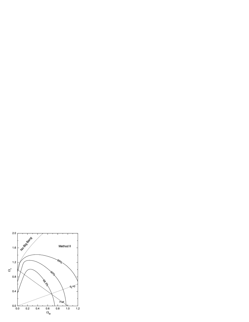
Figure 3: Joint confidence intervals (68.3%, 90% and 99%) in the $\Omega_{M}-\Omega_{\Lambda}$ plane from the 17 GRBs with Method II.

The constraints with Method I are shown in Fig 2 (solid contours). In the concordance model of $\Omega_{M}=0.27$, we find a $\chi^{2}_{dof}=17.91/15=1.19$. We measure $\Omega_{M}=0.15^{+0.45}_{-0.13}$ ($1\sigma$) for a flat $\Lambda$CDM universe. DLX04 proposed Method II based on the principle that if there are unknown cosmology-independent parameters in the $\chi^{2}$ statistic, they are usually marginalized over (i.e. integrating the parameters according to their probability distribution). Note that DLX04 let the parameter $a$ of the Ghirlanda relation intrinsically equal to 1.50. For the purpose of universality, in this paper we let it vary freely, similar to the parameter $C$ of this relation (see details in $\S 2.1$). The constraints with Method II are shown in Fig 3 (solid contours). This method provides a more stringent constraint of $0.14<\Omega_{M}<0.69$ ($1\sigma$) for a flat universe.

By Method I, we recalibrate the Ghirlanda relation for each cosmology, i.e., $\Omega_{M}$ and $\Omega_{\Lambda}$ taken from 0 to 1. We find the half-opening angles of all the bursts are less than 0.23 rad, and that the mean $\sigma_{a}/a$ and $\sigma_{C}/C$ are 0.049 and 0.083. As a result, the typical error terms in Eq. (8) are $\sigma_{S_{\gamma}}/2S_{\gamma}\sim 0.052$, $\sigma_{k}/2k\sim 0.025$, $[\sqrt{C_{\theta}}/(2-2\sqrt{C_{\theta}})](3\sigma_{t_{j}}/t_{j})\sim 0.091$, $[\sqrt{C_{\theta}}/(2-2\sqrt{C_{\theta}})](\sigma_{n_{0}}/n_{0})\sim 0.118$, $[1/(2-2\sqrt{C_{\theta}})](\sigma_{C}/C)\sim 0.055$, $a[1/(2-2\sqrt{C_{\theta}})](\sigma_{E_{p}^{obs}}/E_{p}^{obs})\sim 0.168$, and $\sigma_{a}[1/(2-2\sqrt{C_{\theta}})]\left|{\ln[E_{p}^{obs}(1+z)/100]}\right|\sim 0.056$. These error terms give a typical uncertainty of apparent DM $\sigma_{\mu_{{\rm{obs}}}}\sim 0.5$ magnitudes, which is a factor of $\sim 2$ larger than that derived from the SN Ia gold sample.

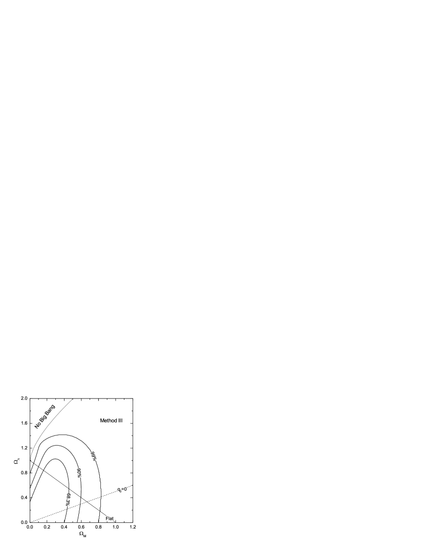
Figure 4: Joint confidence intervals (68.3%, 90% and 99%) in the $\Omega_{M}-\Omega_{\Lambda}$ plane from the 17 GRBs with Method III.

Firmani et al. (2005) proposed the Bayesian approach to use GRBs as cosmic rulers. Being different from their work, we redefined the conditional probability in their method and called it Method III in this paper. The constraints on cosmological parameters with this method are shown in Fig 4 (solid contours). Compared with previous two methods, Method III does give much more stringent confidence intervals at the same confidence levels (C.L.). The results are inspiring and demonstrate the advantages of high-$z$ distance indicators in constraining cosmological parameters. The data set is consistent with the concordance model of $\Omega_{M}=0.27$, yielding a $\chi^{2}_{dof}=19.08/15=1.27$. We also find $0.16<\Omega_{M}<0.45$ ($1\sigma$) for a flat universe.

4 Simulations and Cosmological Constraints

4.1 Procedure of Simulations

As discussed above, the method for the GRB cosmology is different from that for the SN cosmology due to the lack of the low-$z$ calibration. The low-$z$ calibration shall greatly enhance the cosmographic capability of GRBs (assuming no cosmic evolution for the Ghirlanda relation). Therefore, one may ask: could a large high- $z$ GRB sample effectively measure cosmology? To answer this question, we carry out a Monte Carlo simulation and use a large simulated sample to investigate the cosmographic capabilities in different scenarios.

Our simulations are based on the Ghirlanda relation which is calibrated for $\Omega_{M}=0.27$ and $\Omega_{\Lambda}=0.73$. Making use of the sample in Table 1, we find $a=1.53$, $C=0.97$, $\theta<0.2$ rad, and $\log(E_{\gamma}/1\,{\rm erg})\in[49.82,51.96]$. We also find $\log(E^{obs}_{p}/1\,{\rm KeV})\in[1.54,2.89]$. These restrictive conditions are imposed upon our simulations. Each simulated GRB is characterized by a set of $S^{\prime}_{b}$, $t^{\prime}_{j}$, $n^{\prime}$, $z$ and $E^{\prime}_{p}$, where $S^{\prime}_{b}$ is the bolometric fluence.

The simulation procedure is as follows:

(1) We consider the lognormal distributions for the observables $S_{b}$, $t_{j}$ and $n$. From the 17 GRBs, we find $\left\langle{\log\left({S_{b}/1\,\rm{erg}\,{\rm cm}^{-2}}\right)}\right\rangle\sim-4.46$ with $\sigma_{\log\left({S_{b}/1\,\rm{erg}\,{\rm cm}^{-2}}\right)}\sim 0.78$, and $\left\langle{\log\left({t_{j}/1\,{\rm{day}}}\right)}\right\rangle\sim 0.17$ with $\sigma_{\log\left({t_{j}/1\,{\rm{day}}}\right)}\sim 0.27$. Because $n$ is unavailable in the literature for most GRBs, we take $\left\langle{\log\left({n/1\,{\rm{cm}}^{-3}}\right)}\right\rangle\sim 0.40$ with $\sigma_{\log\left({n/1\,{\rm{cm}}^{-3}}\right)}\sim 0.25$. The observable $z$ is selected according to its observational distribution cut by an upper limit $z\sim 4.5$, which is shown in Fig 5. The uncertainty of $z$ is ignored.

(2) We also consider the lognormal distributions for the fractional uncertainties of the observables $S_{b}$, $t_{j}$, $n$ and $E_{p}$. From the observed sample, we find $\left\langle{\log\left({\sigma_{S_{b}}/S_{b}}\right)}\right\rangle\sim-0.97$ with $\sigma_{\log[{\sigma_{S_{b}}/S_{b}}]}\sim 0.16$, $\left\langle{\log\left({\sigma_{t_{j}}/t_{j}}\right)}\right\rangle\sim-0.91$ with $\sigma_{\log[{\sigma_{t_{j}}/t_{j}}]}\sim 0.45$, $\left\langle{\log\left({\sigma_{n}/n}\right)}\right\rangle\sim-0.30$ with $\sigma_{\log[{\sigma_{n}/n}]}\sim 0.10$, and $\left\langle{\log\left({\sigma_{E_{p}}/E_{p}}\right)}\right\rangle\sim-0.83$ with $\sigma_{\log[{\sigma_{E_{p}}/E_{p}}]}\sim 0.26$, respectively. We ensure in code that the fractional uncertainties of the observables $S_{b}$, $t_{j}$, $n$ and $E_{p}$ are less than $25\%$, $35\%$, $100\%$ and $35\%$, respectively.

(3) We simulate a GRB characterized by a set of ($S_{b}\pm\sigma_{S_{b}}$, $t_{j}\pm\sigma_{t_{j}}$, $n\pm\sigma_{n}$ and $z$) according to the distributions that these parameters follow, compute its $E_{\gamma}$ in the cosmic model of $\Omega_{M}=0.27$ and $\Omega_{\Lambda}=0.73$, and then calculate its $E_{p}$ by the Ghirlanda relation of $(E_{\gamma}/10^{50}{\rm ergs})=0.97({E_{p}/100\rm keV})^{1.53}$.

(4) The GRB generated in step (3) follows the “rigid” Ghirlanda relation. We add a random deviation to each parameter, except for $z$, to make this burst more realistic, i.e., $S^{\prime}_{b}=S_{b}+1.1(-1)^{m}\sigma_{S_{b}}$, $t^{\prime}_{j}=t_{j}+1.1(-1)^{m}\sigma_{t_{j}}$, $n^{\prime}=n+1.1(-1)^{m}\sigma_{n}$ and $E_{p}^{\prime}=E_{p}+1.1(-1)^{m}\sigma_{E_{p}}$, where $m$ is randomly taken from 0 and 1.

(5) Using the parameters $S^{\prime}_{b}$, $t^{\prime}_{j}$, $n^{\prime}$, $z$, and $E_{p}^{\prime}$, we compute the parameters $\theta^{\prime}$ and $E^{\prime}_{\gamma}$ for $\Omega_{M}=0.27$ and $\Omega_{\Lambda}=0.73$, and the quantity $E^{\prime\,obs}_{p}=E^{\prime}_{p}/(1+z)$.

(6) Since $\theta<0.2$ rad, $\log(E_{\gamma}/1\,{\rm erg})\in[49.82,51.96]$ and $\log(E^{obs}_{p}/1\,{\rm KeV})\in[1.54,2.89]$ are valid for the observed sample, we require that $\theta^{\prime}$, $\log(E^{\prime}_{\gamma}/1\,{\rm erg})$, and $\log(E^{\prime\,obs}_{p}/1\,{\rm KeV})$ of a simulated GRB must be within the corresponding ranges.

(7) Repeat steps (3)-(6) to generate a sample of 80 bursts.

The half-opening angles of the simulated sample are less than 0.23 rad when $\Omega_{M}$ and $\Omega_{\Lambda}$ are taken from 0 to 1, as in the observed sample. We carry out a circular operation to achieve the simulated sample, which may be established in the Swift era.

4.2 Constraints from Simulated GRBs

By Method I, we find the typical $\sigma_{a}/a$ and $\sigma_{C}/C$ for the large sample decrease to 0.02 and 0.05. This is because for the small observed sample, the dispersion of the Ghirlanda relation is mainly contributed by a few “outliers”, while for the large simulated sample, the bursts are distributed around the “rigid” Ghirlanda relation with a Gaussian distribution (see $\S 4.1$). Such a large sample seems to be more realistic.

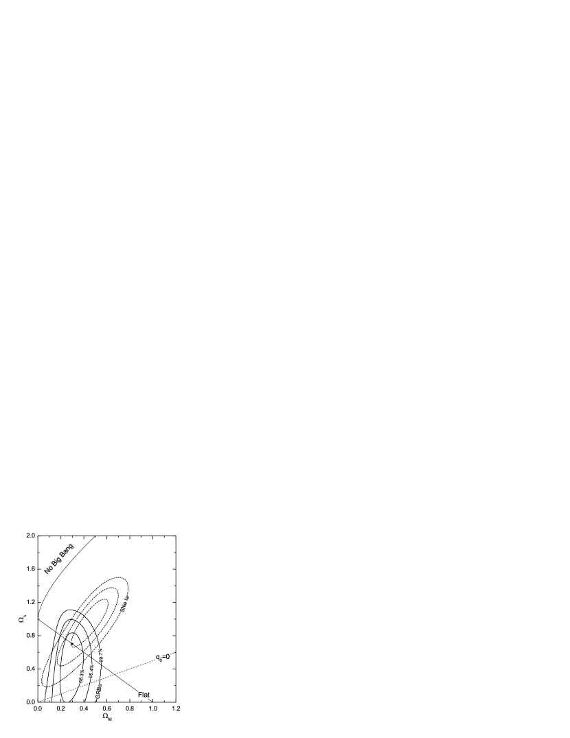
Figure 6: Joint confidence intervals (68.3%, 95.4% and 99.7%) in the $\Omega_{M}$-$\Omega_{\Lambda}$ plane from the 80 simulated GRBs in this work (solid contours) and from the 157 SNe Ia in Riess et al. (2004) (dashed contours). The black dot marks $\Omega_{M}=0.30$ and $\Omega_{\Lambda}=0.70$.

Among several scenarios, we only perform to what degree the simulated sample can constrain the $\Omega_{M}-\Omega_{\Lambda}$ parameters with Method III. The results are shown by solid confidence intervals in Fig 6. Also shown are the constraints derived from the SN gold sample (dashed contours) at the same confidence levels. The main points revealed by this figure are: (1) A large high-$z$ GRB sample could effectively measure cosmology. The simulated GRB data are consistent with the concordance model of $\Omega_{M}\approx 0.3$, yielding a $\chi^{2}_{dof}=94./78.\approx 1.20$. With the prior of a flat universe, the mass density is $\Omega_{M}=0.30^{+0.09}_{-0.06}$ at the $68.3\%$ level. (2) GRBs can well constrain $\Omega_{M}$ rather than $\Omega_{\Lambda}$ due to their high redshifts. The orientation of the elliptical contours is almost vertical to the $\Omega_{M}$ axis. This is an advantage of GRBs over SNe Ia for the cosmological use. (3) GRBs supply complemental content to the SN cosmology. The 157 SNe Ia provide evidence of cosmic acceleration at a very high confidence level. A large GRB sample would reach a similar conclusion. Alone the SN sample nearly rules out the flat universe model at $1\sigma$ level, but a combination of GRBs and SNe makes the concordance model of $\Omega_{M}\approx 0.3$ more favored and thus more agreement with the conclusion from WMAP observations (Spergel et al. 2003).

If the low-$z$ calibration is realized for GRBs, then the solid confidence regions in Fig 6 will become smaller so that they lie in the part of cosmic acceleration at a high C.L. in the $\Omega_{M}-\Omega_{\Lambda}$ plane (not shown in this work). We here present a rough estimation of the detection rate of low-$z$ bursts in the Swift era. Taking $\Omega_{M}=0.27$, $\Omega_{\Lambda}=0.73$, and $h=0.71$, the observed rate of bursts with redshift less than $z$ is

$$\frac{{dN}}{{dt}}=\int_{0}^{z}{dz\frac{{dV(z)}}{{dz}}}\frac{{R_{GRB}(z)}}{{1+z}},$$ (17)

where $R_{GRB}(z)$ is the comoving GRB rate density, and $dV(z)/dz$ is the isotropic comoving volume element,

$$\frac{{dV}}{{dz}}=4\pi\left[{\int_{0}^{z}{\frac{{dz^{\prime}}}{{\sqrt{\Omega_{M}(1+z^{\prime})^{3}+\Omega_{\Lambda}}}}}}\right]^{2}\frac{1}{{\sqrt{\Omega_{M}(1+z)^{3}+\Omega_{\Lambda}}}}.$$ (18)

We assume $R_{GRB}(z)\propto R_{SN}(z)\propto R_{SF}(z)$, where $R_{SN}(z)$ and $R_{SF}(z)$ are the comoving rate densities of core-collapse supernovae and star formation, respectively (Porciani & Madau 2001). We also assume the constant fraction $k=R_{GRB}/R_{SN}\sim 10^{-5}$, which considers the GRB formation efficiency out of the core-collapse SNe and the GRB beaming effect. Additionally, we take $R_{SN}(z)\simeq 0.01R_{SF}(z)\,{\rm M^{-1}_{\bigodot}}$. The global star formation rate for the Einstein-de Sitter universe (Steidel et al. 1999) is

$$R_{SF}(z)=0.16\frac{{\exp(3.4z)}}{{\exp(3.4z)+22}}\,\,\,{\rm{M_{\bigodot}\,yr}}^{{\rm{-1}}}{\rm{Mpc}}^{{\rm{-3}}}.$$ (19)

Thus, we derive the detective probability of low-$z$ GRBs in the Swift era (2$-$4 years): when $z\leq 0.1$, there will be $<1$ burst; and when $z\leq 0.2$, there will be a few bursts. These results agree with the present observational GRB data. In addition, taking into account possible different origins of very low-$z$ bursts (e.g. GRB980425) and high-$z$ bursts, it might not be valid to directly apply the low-$z$ calibrated relation to a high-$z$ sample. However, if the cosmic evolution of the “standard candle” relation is ignored, then in the future one could consider a sample of GRBs with redshift $z\leq 0.2$ for the low-$z$ calibration. As the zero-order approximation, the theoretical luminosity distance of such a GRB sample can be written as $d_{L}(z)=z(c/H_{0})$.

5 Conclusions and Discussion

At present, GRBs with known redshifts are about 45 out of a few thousands, among which 17 are available to derive the Ghirlanda relation. This relation is so tight that it has been considered for the cosmological use. Although the low-$z$ calibration of the Ghirlanda relation is not realized, the observed 17 high-$z$ bursts still provide interesting and even inspiring results. We find GRBs independently place a constraint on the mass density $0.16<\Omega_{M}<0.45$ ($1\sigma$) for a flat $\Lambda$CDM model.

GRBs are becoming more and more standardized candles. Through the Ghirlanda relation, the mean scatter in GRBs is a factor of $\sim 2$ larger than that in SNe Ia. However, the disadvantage of larger scatter in GRBs is compensated, to some extent, by their advantages of high redshifts and immunity to the dust extinction. The shape of the constraints in Fig 6 implies that GRBs could not only measure the mass density $\Omega_{M}$ but also provide complementarity to the SN cosmology. The Swift satellite is hopeful to establish a large GRB sample with known redshifts, perhaps including low-$z$ bursts. In this sense, the GRB cosmology now lies in its babyhood.

A reliable theoretical basis of the Ghirlanda relation is also important for GRBs as a cosmic ruler. Using the small angle approximation for all bursts, a scaling analysis gives $E_{\gamma}\propto{E^{a}_{p}}$ ($a\sim 1.5$) as long as the parameters such as the spectral index $p$ of the distribution of accelerated electrons, the the energy equipartition factor $\varepsilon_{e}$ of the electrons, the energy equipartition factor $\varepsilon_{B}$ of magnetic field, the bulk Lorentz factor $\gamma$, etc., or their combinations are clustered (Zhang & Mészáros 2002; Dai & Lu 2002; Wu, Dai & Liang 2004). This power-law relation could also be understood by the emissions from off-axis relativistic jets (Yamazaki, Ioka & Nakamura 2004; Eichler & Levinson 2004; Levinson & Eichler 2005) and the dissipative photosphere model (Rees & Mészáros 2005). Different plausible explanations imply that this topic needs further investigations.

It should be pointed out that the Ghirlanda relation is obtained under the framework of the uniform top-hat jet model. Other input assumptions include the uniform circumburst medium density $n$ and the constant efficiency $\eta_{\gamma}$ of converting the initial ejecta’s kinetic energy into $\gamma$-ray energy release. However, $n$ and $\eta_{\gamma}$ should be different from burst to burst, and $n$ is variable for a burst in the wind environment (Dai & Lu 1998; Chevalier & Li 1999). Thus, the quantity $n\eta_{\gamma}$ in the Ghirlanda relation might not be clustered for the observed bursts (Friedman & Bloom 2004). New relations with as few well-observed quantities as possible are required for improvement. In this paper, for those bursts with unknown $n$, we assumed $n\simeq 3\,{\rm cm}^{-3}$ as the median value of the distribution of the measured densities, together with a constant fractional uncertainty of $80\%$ (Ghirlanda et al. 2004a; DLX04). We also treat $\eta_{\gamma}=0.2$ and $\sigma_{\eta_{\gamma}}=0$ for all the 17 bursts.

Finally, the Ghirlanda relation is not valid for all the observed BATSE sample. This implies that this relation may suffer from the data selection effect (Band & Preece 2005). Its validity will be tested by the ongoing observations of the Swift mission. However, no matter whether the low-$z$ sample is established or not, the GRB cosmology is expected to progress much in the coming years.

Table 1: Sample of 17 GRBs

GRB	$z$	$E_{p}^{obs}(\sigma_{E_{p}}^{obs})$	$[\alpha,\beta]$	$S_{\gamma}(\sigma_{S_{\gamma}})$	bandpass	$t_{\rm j}(\sigma_{t_{\rm j}})$	$n(\sigma_{n})$	$\eta_{\gamma}$	References	Detected
		[KeV]		[$10^{-6}$ erg cm-2]	[KeV]	days	[cm-3]		($z$, $E_{p}^{obs}$, $[\alpha,\beta]$, $S_{\gamma}$, $t_{\rm jet}$, $n$)	by
grb970828	0.9578	297.7[59.5]	-0.70, -2.07	96.0[9.6]	20-2000	2.2(0.4)	3.0[2.4]	0.2	01,18,18,26,01,no	BATSE
grb980703	0.966	254.0[50.8]	-1.31, -2.40	22.6[2.26]	20-2000	3.4(0.5)	28.0(10.0)	0.2	02,18,18,26,27,27	BATSE
grb990123	1.600	780.8(61.9)	-0.89, -2.45	300.0(40.0)	40-700	2.04(0.46)	3.0[2.4]	0.2	03,19,19,19,28,no	SAX
grb990510	1.619	161.5(16.0)	-1.23, -2.70	19.0(2.0)	40-700	1.57(0.03)	0.29(0.14)	0.2	04,19,19,19,29,41	SAX
grb990705	0.8424	188.8(15.2)	-1.05, -2.20	75.0(8.0)	40-700	1.0(0.2)	3.0[2.4]	0.2	05,19,19,19,30,no	SAX
grb990712	0.4331	65.0(10.5)	-1.88, -2.48	6.5(0.3)	40-700	1.6(0.2)	3.0[2.4]	0.2	06,19,19,19,31,no	SAX
grb991216	1.020	317.3[63.4]	-1.23, -2.18	194.0[19.4]	20-2000	1.2(0.4)	4.7(2.8)	0.2	07,18,18,26,32,41	BATSE
grb011211	2.140	59.2(7.6)	-0.84, -2.30	5.0[0.5]	40-700	1.56(0.02)	3.0[2.4]	0.2	08,20,20,26,33,no	SAX
grb020124	3.200	120.0(22.6)	-1.10, -2.30	6.8[0.68]	30-400	3.0(0.4)	3.0[2.4]	0.2	09,21,21,21,34,no	HETE-2
grb020405	0.690	192.5(53.8)	0.00, -1.87	74.0(0.7)	15-2000	1.67(0.52)	3.0[2.4]	0.2	10,22,22,22,22,no	SAX
grb020813	1.255	212.0(42.0)	-1.05, -2.30	102.0[10.2]	30-400	0.43(0.06)	3.0[2.4]	0.2	11,21,21,21,35,no	HETE-2
grb021004	2.332	79.8(30.0)	-1.01, -2.30	2.55(0.60)	2 -400	4.74(0.14)	30.0(27.0)	0.2	12,23,23,23,36,42	HETE-2
grb021211	1.006	46.8(5.5)	-0.805,-2.37	2.17(0.15)	30-400	1.4(0.5)	3.0[2.4]	0.2	13,24,24,24,37,no	HETE-2
grb030226	1.986	97.1(20.0)	-0.89, -2.30	5.61(0.65)	2 -400	1.04(0.12)	3.0[2.4]	0.2	14,23,23,23,38,no	HETE-2
grb030328	1.520	126.3(13.5)	-1.14, -2.09	36.95(1.40)	2 -400	0.8(0.1)	3.0[2.4]	0.2	15,23,23,23,39,no	HETE-2
grb030329	0.1685	67.9(2.2)	-1.26, -2.28	110.0(10.0)	30-400	0.48(0.03)	1.0(0.11)	0.2	16,25,25,25,40,43	HETE-2
xrf030429	2.658	35.0(9.0)	-1.12, -2.30	0.854(0.14)	2 -400	1.77(1.0)	3.0[2.4]	0.2	17,23,23,23,17,no	HETE-2

References. — (1) Djorgovski et al. 2001; (2) Djorgovski et al. 1998; (3) Kulkarni et al. 1999; (4) Vreeswijk et al. 2001; (5) Le Floc’h et al. 2002; (6) Vreeswijk et al. 2001; (7) Piro et al. 2000; (8) Holland et al. 2002; (9) Hjorth et al. 2003; (10) Price et al. 2003a; (11) Barth et al. 2003; (12) Matheson et al. 2003; (13) Vreeswijk et al. 2003; (14) Greiner et al. 2003a; (15) Rol et al. 2003; (16) Greiner et al. 2003b; (17) Jakobsson, et al. 2004; (18) Jimenez et al. 2001; (19) Amati et al. 2002; (20) Amati 2004; (21) Barraud et al. 2003; (22) Price et al. 2003a; (23) Sakamoto et al. 2004b; (24) Crew et al. 2003; (25) Vanderspek et al. 2004; (26) Bloom et al .2003; (27) Frail et al. 2003; (28) Kulkarni et al. 1999; (29) Stanek et al. 1999; (30) Masetti et al. 2000; (31) Bjornsson et al. 2001; (32) Halpern et al. 2000; (33) Jakobsson et al. 2003; (34) Berger et al. 2002; (35) Barth et al. 2003; (36) Holland et al. 2003; (37) Holland et al. 2004; (38) Klose et al. 2004; (39) Andersen et al. 2003; (40) Price et al. 2003b; (41) Panaitescu & Kumar 2002; (42) Schaefer et al. 2003; (43) Tiengo et al. 2003

Figure 2: Joint confidence intervals (68.3%, 90% and 99%) in the $\Omega_{M}-\Omega_{\Lambda}$ plane from the 17 GRBs with Method I.

Figure 5: Histogram for the redshifts of 80 simulated GRBs, following the redshift distribution of the GRBs observed sofar.

References

- (1) Allen, S. W. et al. 2003 MNRAS 342, 287
- (2) Amati, L. et al. 2002, A&A, 390, 81
- (3) Amati, L. 2004, astro-ph/0405318
- (4) Andersen, M. I. et al. 2003, GCN, 1993
- (5) Atteia, J. L. 2003, A&A, 407, L1
- (6) Barraud, C. et al. 2003, A&A, 400, 1021
- (7) Barth, A. J. et al. 2003, ApJ, 584, L47
- (8) Band, D.L., Matteson, J., Ford, L., et al. 1993, ApJ, 413, 281
- (9) Band, D. L. & Preece, R. D. 2005, ApJ, 627, 2
- (10) Bennett, C. L. et al. 2003, ApJS, 148, 1
- (11) Berger, E. et al. 2002, ApJ, 581, 981
- (12) Berger, E. et al. 2003, Nature, 426, 154
- (13) Bjornsson G. et al. 2001, ApJ, 552, L121
- (14) Bloom, J. S., Frail, D. A., & Sari, R. 2001, AJ, 121, 2879
- (15) Bloom, J. S., Frail, D. A., & Kulkarni, S. R. 2003, ApJ, 594, 674
- (16) Bromm, V., & Loeb, A. 2002, ApJ, 575, 111
- (17) Carroll, S. M., Press, W. H., & Turner, E. L. 1992, ARA&A, 30, 499
- (18) Chevalier, R. A. & Li, Z. Y. 1999, ApJ, 520, L29
- (19) Ciardi, B., & Loeb, A. 2000, ApJ, 540, 687
- (20) Crew, G. B. et al. 2003, ApJ, 599, 387
- (21) Dai, Z. G., & Lu, T. 1998, MNRAS, 298, 87
- (22) Dai, Z. G., & Lu, T. 2002, ApJ, 580, 1013
- (23) Dai, Z. G., Liang, E. W. & Xu, D. 2004, ApJ, 612, L101 (DLX04)
- (24) Djorgovski, S. G. et al. 1998, ApJ, 508, L17
- (25) Djorgovski, S. G. et al. 2001, ApJ, 562, 654
- (26) Eichler, D., & Levinson, A. 2004, ApJ, 614, L13
- (27) Fenimore, E. E. & Ramirez-Ruiz E. 2000, astro-ph/0004176
- (28) Firmani, C., Ghisellini, G., Ghirlanda, G. & Avila-Reese, V. 2005, MNRAS, 360, 1 (FGGA05)
- (29) Frail, D. A., Waxman, E., and Kulkarni, S. R. 2000, ApJ, 537, 191
- (30) Frail, D. A. et al. 2001, ApJ, 562, L55
- (31) Frail, D. A. et al. 2003, ApJ, 590, 992
- (32) Friedman, A. S. & Bloom, J. S., ApJ accepted, (astro-ph/0408413; FB04)
- (33) Fruchter, A. et al. 1999, ApJ, 519, L13
- (34) Galama, T. J. et al. 1998, ApJ, 497, L13
- (35) Ghirlanda, G., Ghisellini, G., & Lazzati, D. 2004a, ApJ, 616, 331
- (36) Ghirlanda, G., Ghisellini, G., Lazzati, D. & Firmani, C. 2004b, ApJ, 613, L13 (GGLF04)
- (37) Gou, L. J., Mészáros, P., Abel, T. & Zhang, B. 2004, ApJ, 604, 508
- (38) Greiner, J. et al. 2003a, GCN, 1886
- (39) Greiner, J. et al. 2003b, GCN, 2020
- (40) Halpern, J. P., et al. 2000, ApJ, 543, 697
- (41) Hjorth, J. et al. 2003, ApJ, 597, 699
- (42) Holland, et al. 2002, AJ, 124, 639
- (43) Holland, et al. 2003, AJ, 125, 2291
- (44) Holland, et al. 2004, astro-ph/0405062
- (45) Jakobsson, P. et al. 2003, A&A, 408, 941
- (46) Jakobsson, P. et al. 2004, A&A, 427, 785
- (47) Jimenez, R., Band, D. L., & Piran, T., 2001, ApJ, 561, 171
- (48) Klose, S. et al. 2004, AJ, 128, 1942
- (49) Knop et al. 2003, ApJ, 598, 102
- (50) Kulkarni, S. R. et al. 1999, Nature, 398, 389
- (51) Lamb, D. Q., & Reichart, D. E. 2000, ApJ, 536, 1
- (52) Lamb, D. Q. et al. 2004, NewA Rev., 48, 423
- (53) Le Floc’h, E. 2002, ApJ, 581, L81
- (54) Liang, E. W., Dai, Z. G., & Wu, X. F. 2004, ApJ, 606, L29
- (55) Liang, E. W. & Zhang B. 2005, ApJ submitted (astro-ph/0504404)
- (56) Lloyd-Ronning, N. M., & Petrosian, V. 2002, ApJ, 565, 182
- (57) Lloyd-Ronning, N. M., & Ramirez-Ruiz, E. 2002, ApJ, 576, 101
- (58) MacFadyen, A.I., & Woosley, S. E. 1999, ApJ, 524, 262
- (59) Masetti, N. et al. 2000, A&A, 354, 473
- (60) Matheson, T. et al. 2003, ApJ, 582, L5
- (61) Norris, J. P. et al. 2000, ApJ, 534, 248
- (62) Panaitescu, A., & Kumar, P. 2002, ApJ, 571, 779
- (63) Perlmutter, S. et al. 1999, ApJ, 517, 565
- (64) Porciani, C. & Madau, P. 2001, ApJ, 548, 522
- (65) Piro, L. et al. 2000, Science, 290, 955
- (66) Press, W. H. et al 1999, Numerical Recipes in Fortran, Cambridge University Press, 660-664
- (67) Price, P. A. et al. 2002, ApJ, 573, 85
- (68) Price, P. A. et al. 2003a, ApJ, 589, 838
- (69) Price, P. A. et al. 2003b, Nature, 423, 844
- (70) Porciani, C. & Madau, P. 2001, ApJ, 548, 522
- (71) Rhoads, J. E. 1999, ApJ, 525, 737
- (72) Riess, A. G. et al. 1998, AJ, 116, 1009
- (73) Riess, A. G. et al. 2004, ApJ, 607, 665
- (74) Rol, E. et al. 2003, GCN, 1981
- (75) Sakamoto, T. et al., 2004a, ApJ, 602, 875
- (76) Sakamoto, T. et al., 2004b, astro-ph/0409128
- (77) Sari, R., Piran, T., & Narayan, R. 1998, ApJ, 497, L17
- (78) Sari, R., Piran, T., & Halpern, J. P. 1999, ApJ, 519, L17
- (79) Sazonov, S. Y. et al. Nature 430, 646
- (80) Schaefer, B. E. 2003, ApJ, 583, L67 (S03)
- (81) Schmidt, B. P. et al. 1998, ApJ, 507, 46
- (82) Soderberg, A. M. et al. Nature 430, 648
- (83) Spergel, D. N. et al. 2003, ApJS, 148, 175
- (84) Stanek, K. Z. et al. 1999, ApJ, 522, L39
- (85) Steidel, C. C. et al. 1999, ApJ, 519, 1
- (86) Tegmark, M. et al. 2004, Phys. Rev. D, 69, 103501
- (87) Tiengo, A. et al. 2003, A&A, 409, 938
- (88) Vanderspek, R. et al. 2004, AJ, 617, 1251
- (89) van den Bergh, S., & Pazder, J. 1992, ApJ, 390, 34
- (90) Vreeswijk, P. M. et al. 2001, ApJ, 546, 672
- (91) Vreeswijk, P. M. et al. 2003, GCN, 1785
- (92) Wu, X. F., Dai, Z. G., & Liang, E. W. 2004, ApJ, 615, 359
- (93) Xu, D. 2005, ApJ submitted (astro-ph/0504052)
- (94) Yamazaki, R., Ioka, K., & Nakamura, T. 2004, ApJ, 606, L33
- (95) Yonetoku, D. et al. 2004, ApJ, 609, 935
- (96) Zhang, B. & Mészáros, P. 2002, ApJ, 581, 1236