A model of rotating hotspots for 3:2 frequency ratio of HFQPOs in black hole X-ray binaries

Abstract

We propose a model to explain a puzzling 3:2 frequency ratio of high frequency quasi-periodic oscillations (HFQPOs) in black hole (BH) X-ray binaries, GRO J1655-40, GRS 1915+105 and XTE J1550-564. In our model a non-axisymmetric magnetic coupling (MC) of a rotating black hole (BH) with its surrounding accretion disc coexists with the Blandford-Znajek (BZ) process. The upper frequency is fitted by a rotating hotspot near the inner edge of the disc, which is produced by the energy transferred from the BH to the disc, and the lower frequency is fitted by another rotating hotspot somewhere away from the inner edge of the disc, which arises from the screw instability of the magnetic field on the disc. It turns out that the 3:2 frequency ratio of HFQPOs in these X-ray binaries could be well fitted to the observational data with a much narrower range of the BH spin. In addition, the spectral properties of HFQPOs are discussed. The correlation of HFQPOs with jets from microquasars is contained naturally in our model.

1 INTRODUCTION

Quasi-periodic oscillations in X-ray binaries have become a very active research field since the launch of the Rossi X-Ray Timing Explorer (RXTE; Bradt, Rothschild & Swank 1993). A key feature in these sources is that some of high frequency quasi-periodic oscillations (HFQPOs) appear in pairs. Five black hole (BH) X-ray binaries exhibit transient HFQPOs, of which three sources have pairs occurring in GRO J1655-40 (450, 300Hz; Strohmayer 2001a, hereafter S01a; Remillard et al 1999), GRS 1915+105 (168, 113Hz; McClintock & Remillard 2003, hereafter MR03), and XTE J1550-564 (276, 184Hz; Miller 2001; Remillard et al 2002) with a puzzling 3:2 ratio of the upper frequency to the lower frequency. Very recently, the 3:2 frequency ratio (henceforth 3:2 ratio) was discovered in the X-ray outburst of H1743-322 (240, 160Hz; Homan et al. 2004; Remillard et al. 2004). These discoveries give the exciting prospect of determining BH mass and spin, as well as testing general relativity in the strong-field regime.

A number of different mechanisms have been proposed to explain the origin of HFQPO pairs in BH X-ray binaries. Strohmayer (S01a; 2001b) investigated combinations of the azimuthal and radial coordinate frequencies in general relativity to explain the HFQPO pairs in GRO J1655-40 and GRS 1915+105. Wagoner et al. (2001) regarded the HFQPO pairs as fundamental g-mode and c-mode discoseismic oscillations in a relativistic accretion disc. Abramowicz & Kluzniak (2001) explained the pairs in GRO J1655-40 as a resonance between orbital and epicyclic motion of accreting matter. It seems that more than one physical model is required to fit all of the HFQPO observations.

As is well known, the Blandford-Znajek (BZ) process is an effective mechanism for powering jets from AGNs and quasars, and it is also applicable to jet production in microquasars (Blandford & Znajek 1977, Mirabel & Rodrigues 1999). Recently, the magnetic coupling (MC) of a rotating BH with its surrounding disc has been investigated by some authors (Blandford 1999; Li 2000a, 2002a; Wang et al. 2002, hereafter W02), which can be regarded as one of the variants of the BZ process. The MC process can be used to explain a very steep emissivity in the inner region of the disc, which is found by the recent XMM-Newton observation of the nearby bright Seyfert 1 galaxy MCG-6-30-15 (Wilms et al. 2001; Li 2002b; Wang et al. 2003a, hereafter W03a). In addition, we explained the HFQPOs in X-ray binaries based on a model of a rotating hotspot due to the MC of a rotating BH with the inner region of the disc (Wang et al. 2003b, hereafter W03b). However, the 3:2 ratio of HFQPOs has not been discussed by virtue of the MC process.

Very recently, we discussed the condition for the coexistence of the BZ and MC processes, and found that this coexistence always accompanies the screw instability of the magnetic field in BH magnetosphere, provided that the BH spin and the power-law index for the variation of the magnetic field on the disc are greater than some critical values (Wang et al. 2003c, 2004, hereafter W03c and W04, respectively).

In this paper we propose a model to explain the 3:2 ratio of HFQPOs in BH X-ray binaries by virtue of non-axisymmetric MC of a rotating BH with its surrounding accretion disc. The upper frequency arises from a rotating hotspot near the inner edge of the disc, and the lower frequency is produced by the screw instability somewhere away from the inner edge. It turns out that the 3:2 ratio of HFQPOs in GRO J1655-40, GRS 1915+105 and XTE J1550-564 is well fitted by energy transferred in the MC process, where six parameters are used to describe the BH mass, spin and distribution of a non-axisymmetric magnetic field. The 3:2 ratio obtained in our model provides a much narrower range of the BH spin compared with the other models. Furthermore, the jets from these BH binaries are explained naturally by the BZ process coexisting with the MC process.

This paper is organized as follows. In section 2 we give a brief description of our model. In section 3 we fit the upper and lower frequencies of HFQPOs by the inner and outer hotspots co-rotating with the disc. The discussion is focused at the issues of the outer hotspot. A scenario of how the presence of the screw instability leads to the outer hotspot is given. In addition, the time-scale of the screw instability is estimated by using an equivalent R-L circuit, and the spectral properties of HFQPOs are discussed by assuming the existence of corona above the disc. In section 4 we discuss some issues of astrophysical meanings related to the 3:2 ratio. Throughout this paper the geometric units $G=c=1$ are used.

2 DESCRIPTION OF OUR MODEL

We intend to fit the 3:2 ratio of HFQPOs by virtue of an rotating BH surrounded by a magnetized accretion disc based on the following assumptions.

(1) The configuration of the poloidal magnetic field is shown in Fig. 1. The radius $r_{ms}$ indicates the inner edge of the disc, being the innermost stable circular orbit (ISCO) (Novikov & Thorne 1973, hereafter NT73), and $r_{{}_{S}}$ is the radius where the screw instability of the magnetic field might occur, which is related to the angle $\theta_{S}$ by the same mapping relation given in W04. As shown in Fig. 1, $\theta_{S}$ is the angular boundary between the open and closed field lines on the horizon, and $\theta_{L}$ is the lower boundary angle for the closed field lines connecting the BH with the disc. Throughout this paper $\theta_{L}=0.45\pi$ is assumed in calculations.

Figure 1: Poloidal magnetic field connecting a rotating BH with a remote astrophysical load and the surrounding disc.

(2) The poloidal magnetic field on the BH horizon is non-axisymmetric as assumed in W03b, varying with the azimuthal angle $\phi$ as follows (see Fig.2 in W03b),

$$B_{H}^{p}\left(\phi\right)=\sqrt{\left\langle{\left({B_{H}^{p}}\right)^{2}}\right\rangle}f\left(\phi\right),\quad f\left(\phi\right)\equiv\left\{{\begin{array}[]{l}1+\delta,\mbox{ }0<\phi<\Delta\phi,\\ 1,\mbox{ }\Delta\phi\leq\phi\leq 2\pi,\\ \end{array}}\right.$$ (1)

where $\sqrt{\left\langle{\left({B_{H}^{p}}\right)^{2}}\right\rangle}$ is root-mean-square of the poloidal magnetic field over the angular coordinate from $\theta=0$ to $\theta_{L}$. The parameter $\delta$ is used to describe the strength of the bulging magnetic field in the azimuthal region $0<\phi<\Delta\phi$.

(3) The magnetosphere is assumed to be force-free outside the BH and the disc, and the closed magnetic field lines are frozen in the disc. The disc is thin and perfectly conducting, lies in the equatorial plane of the BH with the inner boundary being at ISCO.

(4) The poloidal magnetic field varies as a power law with the radial coordinate of the disc as follows,

$$B_{D}^{p}\propto\xi^{-n},$$ (2)

where $B_{D}^{p}$ represents the poloidal magnetic field on the disc, and the parameter $n$ is the power-law index, and the dimensionless radial coordinate is defined as $\xi\equiv r\mathord{\left/{\vphantom{r{r_{ms}}}}\right.\kern-1.2pt}{r_{ms}}$. The radius $r_{ms}$ is related to the BH mass $M$ and the dimensionless spin parameter $a_{*}\equiv a\mathord{\left/{\vphantom{aM}}\right.\kern-1.2pt}M$ as given in NT73.

(5) The magnetic flux connecting the BH with its surrounding disc takes precedence over that connecting the BH with the remote load. As argued in W03c and W04, assumption 5 is crucial for the coexistence of the BZ and MC processes.

The magnetosphere anchored in a Kerr BH and its surrounding disc is described in Boyer-Lindquist coordinates, in which the following parameters are involved (MacDonald and Thorne 1982, hereafter MT82).

$$\left\{{\begin{array}[]{l}\Sigma^{2}=\left({r^{2}+a^{2}}\right)^{2}-a^{2}\Delta\sin^{2}\theta,\mbox{ }\rho^{2}=r^{2}+a^{2}\cos^{2}\theta,\mbox{ }\\ \Delta=r^{2}+a^{2}-2Mr,\mbox{ }\varpi=\left({\Sigma\mathord{\left/{\vphantom{\Sigma\rho}}\right.\kern-1.2pt}\rho}\right)\sin\theta,\\ \alpha={\rho\sqrt{\Delta}}\mathord{\left/{\vphantom{{\rho\sqrt{\Delta}}\Sigma}}\right.\kern-1.2pt}\Sigma.\\ \end{array}}\right.$$ (3)

In W03b the BZ and MC powers in non-axisymmetic case are related to those in axisymmetic case by

$$P_{BZ}^{NA}=\lambda P_{BZ}^{A},$$ (4)

$$P_{MC}^{NA}=\lambda P_{MC}^{A},$$ (5)

where $P_{BZ}^{NA}$ and $P_{MC}^{NA}$ are the powers in non-axisymmetic case, and $P_{BZ}^{A}$ and $P_{MC}^{A}$ are the powers in axisymmetic case, respectively. The parameter $\lambda$ is expressed in terms of $\delta$ and $\varepsilon\equiv{\Delta\phi}\mathord{\left/{\vphantom{{\Delta\phi}{2\pi}}}\right.\kern-1.2pt}{2\pi}$ by

$$\lambda=\left[{\left({1+\delta}\right)\varepsilon+\left({1-\varepsilon}\right)}\right]^{2}=\left({1+\delta\varepsilon}\right)^{2}.$$ (6)

Similarly, the BZ and MC torques in non-axisymmetic case are related to those in axisymmetic case by

$$T_{BZ}^{NA}=\lambda T_{BZ}^{A},$$ (7)

$$T_{MC}^{NA}=\lambda T_{MC}^{A},$$ (8)

where $T_{BZ}^{NA}$ and $T_{MC}^{NA}$ are the torques in non-axisymmetic case, and $T_{BZ}^{A}$ and $T_{MC}^{A}$ are the torques in axisymmetic case, respectively. The powers $P_{BZ}^{A}$ and $P_{MC}^{A}$, and the torques $T_{BZ}^{A}$ and $T_{MC}^{A}$ are given in W02 as follows.

$${P_{BZ}^{A}}\mathord{\left/{\vphantom{{P_{BZ}^{A}}{P_{0}}}}\right.\kern-1.2pt}{P_{0}}=2a_{*}^{2}\int_{0}^{\theta}{\frac{k\left({1-k}\right)\sin^{3}\theta d\theta}{2-\left({1-q}\right)\sin^{2}\theta}},\quad 0<\theta<\theta_{S},$$ (9)

$${P_{MC}^{A}}\mathord{\left/{\vphantom{{P_{MC}^{A}}{P_{0}}}}\right.\kern-1.2pt}{P_{0}}=2a_{*}^{2}\int_{\theta_{S}}^{\theta}{\frac{\beta\left({1-\beta}\right)\sin^{3}\theta d\theta}{2-\left({1-q}\right)\sin^{2}\theta}},\quad\theta_{S}<\theta<\theta_{L}.$$ (10)

$$\begin{array}[]{l}{T_{BZ}^{A}}\mathord{\left/{\vphantom{{T_{BZ}^{A}}{T_{0}}}}\right.\kern-1.2pt}{T_{0}}=\\ \quad\quad 4a_{*}\left({1+q}\right)\int_{0}^{\theta}{\frac{\left({1-\beta}\right)\sin^{3}\theta d\theta}{2-\left({1-q}\right)\sin^{2}\theta}},\quad 0<\theta<\theta_{S},\end{array}$$ (11)

$$\begin{array}[]{l}{T_{MC}^{A}}\mathord{\left/{\vphantom{{T_{MC}^{A}}{T_{0}}}}\right.\kern-1.2pt}{T_{0}}=\\ \quad\quad 4a_{*}\left({1+q}\right)\int_{\theta_{S}}^{\theta}{\frac{\left({1-\beta}\right)\sin^{3}\theta d\theta}{2-\left({1-q}\right)\sin^{2}\theta}},\quad\theta_{S}<\theta<\theta_{L}.\end{array}$$ (12)

In equations (9)—(12), $k$ and $\beta$ are the ratios of the angular velocities of the magnetic field lines to the angular velocity of the BH horizon in the BZ and MC processes, respectively. The quantity $q\equiv\sqrt{1-a_{*}^{2}}$ is a function of the BH spin, and $P_{0}$ and $T_{0}$ are defined as

$$\left\{{\begin{array}[]{l}P_{0}\equiv\left\langle{\left({B_{H}^{p}}\right)^{2}}\right\rangle M^{2}\approx B_{4}^{2}m_{BH}^{2}\times 6.59\times 10^{28}erg\cdot s^{-1},\\ T_{0}\equiv\left\langle{\left({B_{H}^{p}}\right)^{2}}\right\rangle M^{3}\approx B_{4}^{2}m_{BH}^{3}\times 3.26\times 10^{23}g\cdot cm^{2}\cdot s^{-2},\\ \end{array}}\right.$$ (13)

where $B_{4}$ is the strength of the poloidal magnetic field on the horizon in units of $10^{4}gauss$, and $m_{{}_{BH}}$ is defined as $m_{BH}\equiv M\mathord{\left/{\vphantom{M{M_{\odot}}}}\right.\kern-1.2pt}{M_{\odot}}$.

So far six parameters are involved in our model, in which $m_{{}_{BH}}$ and $a_{*}$ are used for describing the mass and spin of the Kerr BH, and the three parameters, $B_{4}$, $\delta$ and $\varepsilon$ are used for describing the non-axisymmetric magnetic field on the horizon, the power-law index $n$ is for the variation of the magnetic field with the radial coordinate of the disc.

3 INNER AND OUTER HOTSPOTS FOR 3:2 FREQUENCY RATIO

As argued in W03b, the upper frequency of HFQPOs is modulated by an inner hotspot, which corresponds to the maximum of function $F_{QPO}$ as follows,

$$F_{QPO}\equiv{r^{2}F}\mathord{\left/{\vphantom{{r^{2}F}{r_{ms}^{2}}}}\right.\kern-1.2pt}{r_{ms}^{2}}F_{0}=\xi^{2}{\left({F_{DA}+F_{MC}}\right)}\mathord{\left/{\vphantom{{\left({F_{DA}+F_{MC}}\right)}{F_{0}}}}\right.\kern-1.2pt}{F_{0}},$$ (14)

where $F_{DA}$ is the radiation flux due to disc accretion, and $F_{MC}$ is radiation flux arising from the energy transferred from the rotating BH into the inner disc in the MC process. We find that the radial coordinate of the inner hotspot, $\xi_{\max}$, only depends on the parameters $a_{*}$, and $n$, i.e., it is independent of the parameters $m_{{}_{BH}}$, $B_{4}$, $\delta$ and $\varepsilon$. Considering that the hotspot is frozen at the disc, we have the upper frequency $\nu_{QPO}^{upper}$ by substituting $\xi_{\max}$ into the Keplerian angular velocity as follows,

$$\nu_{QPO}=\nu_{0}(\xi^{3\mathord{\left/{\vphantom{32}}\right.\kern-1.2pt}2}\chi_{ms}^{3}+a_{*})^{-1},$$ (15)

where $\nu_{0}\equiv\left({m_{BH}}\right)^{-1}\times 3.23\times 10^{4}Hz$. It turns out that $\nu_{QPO}^{upper}$ depends on the three parameters, $m_{{}_{BH}}$, $a_{*}$ and $n$.

The lower frequency of HFQPOs is fitted by an outer hotspot rotating with the Keplerian angular velocity expressed by equation (15), and a scenario for the production of the outer hotspot is given as follows.

It is well known that the magnetic field configurations with both poloidal and toroidal components can be screw instable (Kadomtsev 1966; Bateman 1978). According to the Kruskal-Shafranov criterion (Kadomtsev 1966), the screw instability will occur, if the toroidal magnetic field becomes so strong that the magnetic field line turns around itself about once. Recently, some authors discussed the screw instability in BH magnetosphere (Gruzinov 1999a; Li 2000b; Tomimatsu et el. 2001). In W04 we suggested that the criterion for the screw instability in the MC process could be expressed by

$$F_{Screw}\left({a_{*};\xi,n}\right)-L\mathord{\left/{\vphantom{L{\left({2\pi\varpi_{D}}\right)}}}\right.\kern-1.2pt}{\left({2\pi\varpi_{D}}\right)}\leq 0,$$ (16)

where $L$ is the poloidal length of the closed field line connecting the BH and the disc, $\varpi_{{}_{D}}$ is the cylindrical radius on the disc, and $F_{Screw}\left({a_{*};\xi,n}\right)$ is a function of $a_{*}$, $\xi$ and $n$.

Setting equality in equation (16), we obtain the critical radial coordinate $\xi_{S}\equiv{r_{S}}\mathord{\left/{\vphantom{{r_{S}}{r_{ms}}}}\right.\kern-1.2pt}{r_{ms}}$ for the screw instability, which depends on the parameters $a_{*}$ and $n$.

It is believed that a disc is probably surrounded by a high-temperature corona analogous to the solar corona (Liang & Price 1977; Haardt 1991; Zhang et al 2000). Very recently, some authors argued that the coronal heating in some stars including the Sun is probably related to dissipation of currents, and very strong X-ray emissions arise from variation of magnetic fields (Galsgaard & Parnell 2004; Peter et al. 2004).

Analogously, if the corona exists above the disc in our model, we expect that the corona above $\xi_{S}$ might be heated by the induced current due to the screw instability of the non-axisymmetric magnetic field. Therefore a very strong X-ray emission would be produced above the rotating outer hotspot, and the lower frequency $\nu_{QPO}^{lower}$ is obtained directly by substituting $\xi_{S}$ into equation (15).

The time-scale of the screw instability can be estimated by using an equivalent circuit as shown in Fig. 2, in which the segments LM and KN represent the two adjacent magnetic surfaces connecting the BH horizon and the outer hotspot as shown in Fig. 2a. Considering the existence of the toroidal magnetic field threading each loop, we introduce an inductor into the circuit, which is represented by the symbol $\Delta L$ in Fig. 2b.

$$\Delta\varepsilon_{H}=\left({{\Delta\Psi^{p}}\mathord{\left/{\vphantom{{\Delta\Psi^{p}}{2\pi}}}\right.\kern-1.2pt}{2\pi}}\right)\Omega_{H},\quad\Delta\varepsilon_{D}=-\left({{\Delta\Psi^{p}}\mathord{\left/{\vphantom{{\Delta\Psi^{p}}{2\pi}}}\right.\kern-1.2pt}{2\pi}}\right)\Omega_{D},$$ (17)

where $\Delta\Psi^{p}$ is the flux of the poloidal magnetic field sandwiched by the magnetic surfaces LM and KN. The resistance at the BH horizon is given by

$$\Delta R_{H}=\sigma_{H}\frac{\Delta l}{2\pi\varpi_{H}}=\frac{2\rho_{H}\Delta\theta_{H}}{\varpi_{H}},$$ (18)

where $\sigma_{H}=4\pi=377ohm$ is the surface resistivity of the BH horizon (MT82), and $\Delta\theta_{H}$ is the angle on the horizon spanned by the two surfaces. The quantities $\rho_{{}_{H}}$ and $\varpi_{{}_{H}}$ are the Kerr metric parameters at the horizon. The inductance $\Delta L$ in the R-L circuit is defined by

$$\Delta L={\Delta\Psi^{T}}\mathord{\left/{\vphantom{{\Delta\Psi^{T}}{I^{p}}}}\right.\kern-1.2pt}{I^{p}},$$ (19)

where $I^{p}$ and $\Delta\Psi^{T}$ are the poloidal current flowing in the circuit and the flux of the toroidal magnetic field threading the circuit, respectively. The flux $\Delta\Psi^{T}$ can be integrated over the region KLMN as follows,

$$\Delta\Psi^{T}=\oint_{loop}{B^{T}\sqrt{g_{rr}g_{\theta\theta}}dr}d\theta,$$ (20)

where the toroidal magnetic field measured by “zero-angular-momentum observers” (ZAMOs) is given as

$$B^{T}={2I^{p}}\mathord{\left/{\vphantom{{2I^{p}}{\left({\alpha\varpi}\right)}}}\right.\kern-1.2pt}{\left({\alpha\varpi}\right)},$$ (21)

where $\alpha$ is the lapse function defined in equation (3).

Unfortunately, the geometric shapes of the magnetic surfaces LM and KN are unknown. As an approximate estimation we assume that the surfaces LM and KN are formed by rotating the two adjacent circles around the symmetric axis, and $\Delta\Psi^{T}$ can be calculated by integrating over the region KLMN as shown in Fig. 3. Finally, we calculate the quantity $\tau\equiv{\Delta L}\mathord{\left/{\vphantom{{\Delta L}{\Delta R_{H}}}}\right.\kern-1.2pt}{\Delta R_{H}}$ by incorporating equations (18)—(21), which is independent of $I^{P}$.

(a)

(b)

Figure 2: (a) Two adjacent magnetic surfaces connecting the BH horizon and the outer hotspot, (b) one loop of equivalent circuit for screw instability.

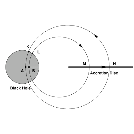
Figure 3: Two adjacent magnetic surfaces produced by two rotating circles, where the arrows represent the current flowing in the R-L circuit.

As a simple analysis we can divide one event of the screw instability into two stages. In stage 1 the instability starts, and the magnetic energy is released rapidly, the poloidal current and thus the toroidal magnetic field decrease to zero in very short time. In stage 2 the toroidal magnetic field recovers gradually with the increasing poloidal current $I^{P}$ in the R-L circuit, until the next event of the instability occurs according to the criterion (16). It seems reasonable that the duration in stage 1 is much less than that in stage 2, and the time-scale of the screw instability depends mainly on the duration of stage 2, which is regarded as the relax time of the poloidal current $I^{P}$ in the R-L circuit. The current $I^{P}$ is governed by the following equation,

$$\Delta L\frac{dI^{P}}{dt}+\Delta R_{H}I^{P}=\Delta\varepsilon_{H}+\Delta\varepsilon_{L}.$$ (22)

Setting the initial condition, $I^{P}=0$, we have the solution,

$$I^{P}\left(t\right)=I_{steady}^{p}\left({1-e^{-t\mathord{\left/{\vphantom{t\tau}}\right.\kern-1.2pt}\tau}}\right),$$ (23)

where $I_{steady}^{p}$ is the steady current in the R-L circuit, and it reads

$$I_{steady}^{p}={\left({\Delta\varepsilon_{H}+\Delta\varepsilon_{L}}\right)}\mathord{\left/{\vphantom{{\left({\Delta\varepsilon_{H}+\Delta\varepsilon_{L}}\right)}{\Delta R_{H}}}}\right.\kern-1.2pt}{\Delta R_{H}}.$$ (24)

From equation (23) we obtain that the poloidal current attains 99.3% of $I_{steady}^{p}$ in the relax time $t_{relax}=5\tau$, implying the recovery of the toroidal magnetic field. Thus the time-scale of the screw instability can be estimated as

$$t_{Screw}>t_{relax}=5\tau.$$ (25)

Summarizing the above results, we have the upper and lower frequencies of HFQPOs, and the corresponding values of $\xi_{\max}$, $\xi_{S}$ and $t_{relax}$ as shown in Table 1. It is easy to check from Table 1 that the time-scale of the screw instability is generally greater than the corresponding periods of HFQPOs, i.e.,

$$t_{Screw}>t_{relax}>1\mathord{\left/{\vphantom{1{\nu_{QPO}^{upper}>1\mathord{\left/{\vphantom{1{\nu_{QPO}^{lower}}}}\right.\kern-1.2pt}{\nu_{QPO}^{lower}}}}}\right.\kern-1.2pt}{\nu_{QPO}^{upper}>1\mathord{\left/{\vphantom{1{\nu_{QPO}^{lower}}}}\right.\kern-1.2pt}{\nu_{QPO}^{lower}}}.$$ (26)

As pointed out in MR03, the spectral properties of accreting black holes in states which show HFQPOs are usually dominated by a steep power-law (SPL) component. However, the origin of X-ray power-law remains controversial. Most of models for the SPL state invoke inverse Compton scattering as the operant radiation mechanism, and the radiation spectrum formed through Comptonization of low-frequency photons in a hot thermal plasma cloud may be described by a power law (Pozdnyakov, Sobol & Syunyaev 1983). It is noted that the origin of the Comptonizing electrons involves magnetic instabilities in the accretion disc (Poutanen & Fabian 1999), with which the screw instability in our model is consistent.

Table 1: The 3:2 ratio of HFQPOs produced by the inner and outer hotspots with $\delta=0.5$ and $\varepsilon=0.2$. Henceforth BHB-I, II and III represent GRO J1655-40, GRS 1915+105 and XTE J1550-564, respectively.

BHB	$a_{*}$	$n$	$m_{{}_{BH}}$	$t_{relax}$ (sec)	Inner Hotspot			Outer Hotspot
					$\xi_{\max}$	${E_{HS}^{upper}}\mathord{\left/{\vphantom{{E_{HS}^{upper}}{B_{4}^{1/2}}}}\right.\kern-1.2pt}{B_{4}^{1/2}}$ (kev)	$\nu_{QPO}^{upper}$ (Hz)	$\xi_{SC}$	${E_{HS}^{lower}}\mathord{\left/{\vphantom{{E_{HS}^{lower}}{B_{4}^{1/2}}}}\right.\kern-1.2pt}{B_{4}^{1/2}}$ (kev)	$\nu_{QPO}^{lower}$ (Hz)
I	0.777	6.22	6.8	$7.61\times 10^{-3}$	1.277	$7.23\times 10^{-3}$	450	2.015	$4.96\times 10^{-3}$	300
	0.730	6.27	5.8	$6.57\times 10^{-3}$	1.281	$6.72\times 10^{-3}$	450	2.097	$4.46\times 10^{-3}$	300
II	0.773	6.23	18	$2.02\times 10^{-2}$	1.277	$7.19\times 10^{-3}$	168	2.021	$4.92\times 10^{-3}$	113
	0.603	6.17	10	$1.11\times 10^{-2}$	1.297	$5.55\times 10^{-3}$	168	2.428	$3.27\times 10^{-3}$	113
III	0.788	6.19	11.5	$1.28\times 10^{-2}$	1.276	$7.37\times 10^{-3}$	276	2.000	$5.09\times 10^{-3}$	184
	0.696	6.29	8.5	$9.72\times 10^{-3}$	1.284	$6.38\times 10^{-3}$	276	2.159	$4.14\times 10^{-3}$	184

Note: The value ranges of the BH mass corresponding to GRO J1655-40, GRS 1915+105 and XTE J1550-564 are adopted from Greene et al. (2001), MR03 and Orosz et al. (2002), respectively.

Suppose that the spectral properties of the inner and outer hotspots arise from blackbody spectra, the effective radiation temperature $\left({T_{HS}}\right)_{eff}$ is expressed by

$$T_{eff}=T_{0}\left[{f_{DA}+f_{MC}}\right]^{1\mathord{\left/{\vphantom{14}}\right.\kern-1.2pt}4},$$ (27)

$$T_{0}=\left({{F_{0}}\mathord{\left/{\vphantom{{F_{0}}\sigma}}\right.\kern-1.2pt}\sigma}\right)^{1\mathord{\left/{\vphantom{14}}\right.\kern-1.2pt}4}\approx 4.8\times 10^{5}B_{4}^{1\mathord{\left/{\vphantom{12}}\right.\kern-1.2pt}2}\left(K\right),$$ (28)

where $\sigma$ is the Stefan-Boltzmann constant. The energy of the inner and outer hotspots can be estimated by

$$E_{HS}\equiv k_{B}T_{eff}=E_{0}\left[{f_{DA}+f_{MC}}\right]^{1\mathord{\left/{\vphantom{14}}\right.\kern-1.2pt}4},$$ (29)

$$E_{0}=k_{B}\left({{F_{0}}\mathord{\left/{\vphantom{{F_{0}}\sigma}}\right.\kern-1.2pt}\sigma}\right)^{1\mathord{\left/{\vphantom{14}}\right.\kern-1.2pt}4}\approx 4.14\times 10^{-2}B_{4}^{1\mathord{\left/{\vphantom{12}}\right.\kern-1.2pt}2}\left({kev}\right),$$ (30)

where $k_{B}$ is the Boltzmann constant. Substituting $\xi_{\max}$ and $\xi_{S}$ into equation (29), we have the energy of the inner and outer hotspots $E_{HS}^{upper}$ and $E_{HS}^{lower}$ as shown in Table 1.

Inspecting equation (29) and the expressions for $f_{DA}$ and $f_{MC}$ given in W03b, we find that both $E_{HS}^{upper}$ and $E_{HS}^{lower}$ depend not only on the parameters, $a_{*}$ and $n$, but also on the parameters for the non-axisymmetric magnetic field, $B_{4}^{1/2}$, $\delta$ and $\varepsilon$. It is worthy to point out that both $E_{HS}^{upper}$ and $E_{HS}^{lower}$ are independent of the BH mass of the X-ray binaries.

4 DISCUSSION

Inspecting Table 1, we find that the 3:2 ratios of HFQPOs in GRO J1655-40, GRS 1915+105 and XTE J1550-564 are well fitted by adjusting the two parameters, $a_{*}$ and $n$, for the given value ranges of $m_{{}_{BH}}$. In this section we discuss some issues of astrophysical meanings related to the 3:2 ratio of HFQPOs in the BH binaries.

4.1 3:2 ratio and magnetic field on the BH horizon

It is pointed out that the twin HFQPOs are not always detected together in GRO J1655-40, i.e., 300 Hz QPO is observed sometimes without 450 Hz detection, while 450 Hz QPO is observed sometimes without 300 Hz detection (S01a). In our model the upper and lower frequencies of HFQPOs are produced by the inner and outer hotspots, which are located at different sites of the disc. In addition, our model is proposed based on the non-axisymmetric magnetic field on the horizon, and two different physical mechanisms are involved, i.e., the MC process for the inner hotspot and the screw instability for the outer hotspot. Since the non-axisymmetric magnetic field cannot be stationary on the horizon, we can understand that the twin HFQPOs do not have to occur simultaneously in some cases.

In Table 1, both $E_{HS}^{upper}$ and $E_{HS}^{lower}$ reach the energy level of emitting X-ray, provided that the root-mean square of the magnetic field on the horizon is strong enough to be $\sim 10^{9}gauss$ ($B_{4}\sim 10^{5})$. Considering that a system cannot radiate a given flux at less than the blackbody temperature (Frank et al. 1992), the strength of magnetic field of $\sim 10^{9}gauss$ might be regarded as a upper limit for energy level of emitting X-ray in BH binaries.

It is pointed out in S01a that the energy spectra of the 300 Hz QPO appear to be significantly different from those of the 450 Hz QPO in GRO J1655-40: The former has a typical amplitude in the 2–12 keV band, while the latter is detected in the hard band, 13–27 keV. It is also shown in Fig. 4.16 of MR03 that the power densities corresponding to the upper frequency are greater than those corresponding to the lower frequency of HFQPOs in some BH X-ray binaries, such as GRO J1655-40 (450, 300Hz) and XTE J1550-564 (276, 184Hz). These observations are consistent with the results obtained in our model, i.e., $E_{HS}^{upper}$ is greater than $E_{HS}^{lower}$ for each BH binary as shown in Table 1.

4.2 BH spin and mass constrained by 3:2 ratio

It is widely believed that HFQPOs in BH binaries might be a unique timing signature constraining the BH mass and spin via a model rooted in general relativity. Thus a precise measurement of the 3:2 ratio of HFQPOs becomes an approach to estimate the BH mass and spin. Combining the fitting results in Table 1 with the observations of the three BH binaries, we discuss the issues related to the BH mass and spin as follows.

The BH spin in GRO J1655-40 has been estimated by some authors. Interpreting the X-ray spectra, Zhang, Cui & Chen (1997) suggested that the most likely value is $0.7<a_{*}<1$, while Sobczak et al. (1999) give an upper limit $a_{*}<0.7$. Assuming that a bright spot appears near the radius of the maximal proper radiation flux from a disc around a rotating BH, Gruzinov (1999b) inferred an upper limit $a_{*}<0.6$ for the BH in GRO J1655-40. Abramowicz & Kluzniak (2001) suggested that the 3:2 ratio in GRO J1655-40 arises from a resonance between orbital and epicyclic motion of accreting matter, and they estimated that the value range of the BH spin is $0.2<a_{*}<0.65$. Compared with the above estimation ranges, we provide a much narrower range for the BH spin in GRO J1655-40, $0.730<a_{*}<0.777$, as shown in Table 1, where the BH spins in GRS 1915+105 and XTE J1550-564 are also constrained in rather narrow ranges, $0.603<a_{*}<0.773$ and $0.696<a_{*}<0.788$, respectively.

4.3 3:2 ratio and jets from microquasars

The BH X-ray binaries, GRO J1655-40, GRS 1915+105 and XTE J1550-564, are also regarded as microquasars, from which relativistic jets are observed (Mirabel & Rodrigues 1998, 1999 and references therein; see also Table 4.2 of MR03). This correlation can be explained very naturally by virtue of the magnetic field configuration as shown in Fig. 1. The jet power is assumed to be provided by the BZ mechanism and expressed by equations (4) and (9). Substituting $a_{*}$, $n$, $m_{{}_{BH}}$ and $\xi_{S}$ into these equations, we have the jet powers as shown in Table 2. In calculations the parameter $k=0.5$ is taken for the optimal BZ power (MT82).

Table 2: The jet powers accompanying 3:2 ratio of HFQPOs with $\delta=0.5$ and $\varepsilon=0.2$.

BHB	$a_{*}$	$n$	$m_{{}_{BH}}$	$\theta_{S}$	${P_{BZ}^{NA}}\mathord{\left/{\vphantom{{P_{BZ}^{NA}}{B_{4}^{2}}}}\right.\kern-1.2pt}{B_{4}^{2}}\left({{erg}\mathord{\left/{\vphantom{{erg}s}}\right.\kern-1.2pt}s}\right)$
I	0.777	6.22	6.8	$50.7^{0}$	$7.09\times 10^{28}$
	0.730	6.27	5.8	$48.9^{0}$	$3.98\times 10^{28}$
II	0.773	6.23	18	$50.5^{0}$	$4.87\times 10^{29}$
	0.603	6.17	10	$42.4^{0}$	$4.68\times 10^{28}$
III	0.788	6.19	11.5	$50.9^{0}$	$2.14\times 10^{29}$
	0.696	6.29	8.5	$47.7^{0}$	$7.01\times 10^{28}$

Mirabel & Rodriguez (1999) pointed out that GRS 1915+105 may have a short-term jet power of $\sim\mbox{10}^{39}{erg}\mathord{\left/{\vphantom{{erg}s}}\right.\kern-1.2pt}s$ in its very high state, which is a large fraction of the observed accretion power. From Table 2 we have the angular boundary and the corresponding BZ power for GRS 1915+105 as follows.

$$P_{BZ}^{NA}=4.87\times 10^{29}B_{4}^{2}\left({{erg}\mathord{\left/{\vphantom{{erg}s}}\right.\kern-1.2pt}s}\right),\quad 0<\theta<50.5^{0},$$ (31)

$$P_{BZ}^{NA}=4.68\times 10^{28}B_{4}^{2}\left({{erg}\mathord{\left/{\vphantom{{erg}s}}\right.\kern-1.2pt}s}\right),\quad 0<\theta_{S}<42.4^{0}.$$ (32)

Equations (31) and (32) imply that a large fraction of the rotating energy is extracted from the BH contained in GRS 1915+105 for the jet power, and $P_{BZ}^{NA}$ can reaches $\sim\mbox{10}^{39}{erg}\mathord{\left/{\vphantom{{erg}s}}\right.\kern-1.2pt}s$, provided that the magnetic field on the horizon is strong enough to attain $\sim 10^{9}gauss$ ($B_{4}\sim 10^{5})$. This strength of the magnetic field is the same as that required by the inner and outer hotspots for emitting X-ray. By using equations (4) and (9) we find that the BZ power increases monotonically with the power-law index $n$ for the given BH spin $a_{*}$, while it varies non-monotonically with $a_{*}$ for the given $n$ as shown in Fig. 4.

   (a)

   (b)

Figure 4: The BZ power $P_{BZ}^{NA}$ (a) varying with $n$ with the given values of $a_{*}$, (b) varying with $a_{*}$ with the given values of $n$.

4.4 3:2 ratio and electric current on disc

As shown in Table 1, a very large power-law index $n$ varying from 6.17 to 6.29 is required by the 3:2 ratio of HFQPOs in the BH binaries. It implies that the poloidal magnetic field increases inward in a very steep way governed by equation (2). It is worthy to point out that this result is consistent with that in W03a, where the power-law index $n$ varying from 6 to 8 is required to explain a very steep emissivity (4-5) observed in Seyfert 1 galaxy MCG-6-30-15.

The poloidal magnetic field arises most probably from the toroidal electric current on the disc, and the current density $j_{\varphi}$ is related to $B_{D}^{p}$ by Ampere’s law as follows.

$$j_{\varphi}=\frac{1}{4\pi}\frac{dB_{D}^{p}}{dr}=\frac{1}{4\pi r_{ms}}\frac{dB_{D}^{p}}{d\xi}=-\frac{n\left({B_{D}^{p}}\right)_{ms}}{4\pi r_{ms}}\xi^{-\left({n+1}\right)}.$$ (33)

Inspecting equation (33), we obtain two features of the toroidal electric current on the disc.

(i) The minus sign in equation (33) shows that the current flows in the opposite direction to the disc matter; (ii) the power-law index $n+1$ in equation (33) implies that the profile of the current density in the central disc is steeper than that of the magnetic field. We give a primary explanation for these features as follows.

Probably the direction of the current arises from the effect of the closed magnetic field lines on the charged particles of the disc matter. In our model the angular velocity of the BH is required to be greater than that of the disc to produce the inner and outer hotspots on the disc. Therefore the charged particles of the disc matter will be dragged forward by the closed field lines. Considering that the mass of the positive charged particle, such as proton, is much greater than that of electron, we think that the bulk flow of electrons might be a little ahead of that of protons. Probably the minute difference in the two kinds of the bulk flows results in a current in the opposite direction to the disc.

On the other hand, the flux of angular momentum transferred from the rotating BH to the disc is given by

$$H_{MC}^{NA}=\frac{\partial{T_{MC}^{NA}}\mathord{\left/{\vphantom{{T_{MC}^{NA}}{\partial r}}}\right.\kern-1.2pt}{\partial r}}{4\pi r}.$$ (34)

Substituting equations (8) and (12) into equation (34), we have

$$\begin{array}[]{l}H_{MC}^{NA}=\frac{1}{4\pi\xi r_{ms}^{2}}\left({{\partial\theta}\mathord{\left/{\vphantom{{\partial\theta}{\partial\xi}}}\right.\kern-1.2pt}{\partial\xi}}\right)\left({\partial{T_{MC}^{NA}}\mathord{\left/{\vphantom{{T_{MC}^{NA}}{\partial\theta}}}\right.\kern-1.2pt}{\partial\theta}}\right)\\ \quad\quad\quad=-\frac{\lambda a_{*}\left({1+q}\right)}{\pi r_{ms}^{2}}\frac{\left({1-\beta}\right)\xi^{-1}\mbox{G}\left({a_{*};\xi,n}\right)}{\left[{2\csc^{2}\theta-\left({1-q}\right)}\right]}.\end{array}$$ (35)

Incorporating equation (2) with equation (35), we have

$$H_{MC}^{NA}\propto\xi^{-n}.$$ (36)

Considering that the flux of angular momentum, $H_{MC}^{NA}$, transferred to the disc will block the accreting particles, and the blocking effect would be much more significant for electrons than protons due to the mass differences. Thus more electrons would stay in the region very close to ISCO. That is why the current density consist of the bulk flow of electrons and it varies with $\xi$ in a power law expressed by equation (33).

As a summary we intend to give a comment for the six parameters involved in our model. The BH mass $m_{{}_{BH}}$ has its range given by observations, and $B_{4}\approx 10^{5}$ is required by the hotspots for emitting X-ray. The parameters $\varepsilon$ and $\delta$ are used to describe the non-axisymmetric magnetic field on the BH horizon. In fact, neither the position nor the energy of the inner and outer hotspots is sensitive to the values of $\varepsilon$ and $\delta$, and we take $\delta=0.5$ and $\varepsilon=0.2$ in calculations. Thus the rest two parameters, $a_{*}$ and $n$ are adjustable in fitting the 3:2 ratio, which play very important roles in fitting the 3:2 ratio of HFQPOs.

In this paper a non-axisymmetric magnetic field on the BH horizon is assumed in an ad hoc way. Unfortunately, we cannot give a good explanation for its existence at present. Probably the non-axisymmetric magnetic field on the BH horizon arises from non-axisymmetric accretion disc, since the magnetic field is brought and held by the surrounding magnetized disc. We hope to approach this difficult task in future.

Acknowledgments. We thank the anonymous referee for his/her many constructive suggestions. This work is supported by the National Natural Science Foundation of China under Grant Numbers 10173004, 10373006 and 10121503.

References

- [1] Abramowicz, M. A., & Kluzniak, W., 2001, A&A, 374, L19
- [2] Bateman G., MHD Instabilities, 1978, (Cambridge: The MIT Press)
- [3] Blandford, R. D., & Znajek, R. L. 1977, MNRAS, 179, 433
- [4] Blandford, R. D., 1999, in ASP Conf. Ser. 160, Astrophysical Discs: An EC Summer School, ed. J. A. Sellwood & J. Goodman (San Francisco: ASP), 265 (B99)
- [5] Bradt, H. V., Rothschild, R. E., & Swank, J. H., 1993, A&AS, 97, 355
- [6] Frank J., King A. R., & Raine D. L., 1992, Accretion Power in Astrophysics, 2nd ed., Cambridge Univ. Press, Cambridge
- [7] Galsgaard, K., & Parnell, C., Procedings of SOHO 15 Coronal Heating, ESA publication, astro-ph/0409562
- [8] Greene, J., Bailyn, C. D., & Orosz, J. A., 2001, ApJ, 554, 1290
- [9] Gruzinov A., 1999a, astro-ph/9908101
- [10] Gruzinov A., 1999b, astro-ph/9910335
- [11] Haardt F., & Maraschi L., 1991, ApJ, 380, L51
- [12] Homan, J., 2004, astro-ph/0406334
- [13] Kadomtsev B. B., 1966, Rev. Plasma Phys., 2, 153
- [14] Liang E. P. T., Price R. H., 1977, ApJ, 218, 247
- [15] Li, L. -X., 2000a, ApJ, 533, L115
- [16] Li, L. -X., 2000b, ApJ, 531, L111
- [17] Li, L. -X., 2002a, ApJ, 567, 463
- [18] Li, L. -X., 2002b, A&A, 392, 469
- [19] Macdonald D., & Thorne K. S., 1982, MNRAS, 198, 345 (MT82)
- [20] McClintock J. E., & Remillard, R. A., 2003, in “Compact Stellar X-ray Sources,” eds. W. H. G. Lewin & M. van der Klis, (Cambridge U. Press), in press; astro-ph/0306213 (MR03)
- [21] Mirabel & Rodrigues, 1998, Nature, 392, 673
- [22] Mirabel & Rodrigues, 1999, ARA&A, 37, 409
- [23] Miller, J. M. et al., 2001, ApJ, 563, 928
- [24] Novikov, I. D., & Thorne, K. S., 1973, in Black Holes, ed. Dewitt C, (Gordon and Breach, New York) p.345
- [25] Orosz et al., 2002, ApJ, 568, 845
- [26] Peter, H., Gudiksen, B., & Nordlund, A., Procedings of SOHO 15 Coronal Heating, ESA publication, astro-ph/0409504
- [27] Poutanen, J., & Fabian, A. C., 1999, MNRAS, 306, L31
- [28] Pozdnyakov, L. A., Sobol, I. M., & Sunyaev, R. A., 1983, in Sov. Sci. Rev./Sec. E: Astr. Space Phys. Rev., Vol. 2, ed. R. A. Sunyaev (New York: Harwood), 189
- [29] Remillard, R. A., et al., 1999, ApJ, 522, 397
- [30] Remillard, R. A., et al., 2002, ApJ, 564, 962
- [31] Remillard, R. A., et al., 2004, astro-ph/0407025
- [32] Sobczak, G. I., et al., 1999, ApJ, 520, 776
- [33] Strohmayer, T. E., 2001a, ApJ, 552, L49
- [34] Strohmayer, T. E., 2001b, ApJ, 554, L169
- [35] Tomimatse A., Matsuoka T., & Takahashi M., 2001, Phys. Rev. D64, 123003
- [36] Wagoner, R. V., Silbergleit, A. S., & Ortega-Rodriguez, M. 2001, ApJ, 559, L25
- [37] Wang, D.-X., Xiao K., & Lei W.-H. 2002, MNRAS, 335, 655 (W02)
- [38] Wang, D.-X., Lei W.-H., & Ma R.-Y., 2003, MNRAS, 342, 851 (W03a)
- [39] Wang D.-X., Ma R.-Y., Lei W.-H., & Yao G.-Z., 2003a, MNRAS, 344, 473 (W03b)
- [40] Wang D.-X., Ma R.-Y., Lei W.-H., & Yao G.-Z., 2003b, ApJ, 595, 109 (W03c)
- [41] Wang D.-X., Ma R.-Y., Lei W.-H., & Yao G.-Z., 2004, ApJ, 601, 1031 (W04)
- [42] Wilms J. et al., 2001, MNRAS, 328, L27
- [43] Zhang, S. N., Cui, W., & Chen W., 1997, ApJ, 482, L155
- [44] Zhang S. N. et al., 2000, Science, 287, 1239