The dark clump near Abell 1942:
dark matter halo or statistical fluke?

Weak lensing surveys provide the possibility of identifying dark matter halos based on their total matter content rather than just the luminous matter content. On the basis of two sets of observations carried out with the CFHT, Erben et al. (2000) presented the first candidate dark clump, i.e. a dark matter concentration identified by its significant weak lensing signal without a corresponding galaxy overdensity or X-ray emission.

We present a set of HST mosaic observations which confirms the presence of an alignment signal at the dark clump position. The signal strength, however, is weaker than in the ground-based data. It is therefore still unclear whether the signal is caused by a lensing mass or is just a chance alignment. We also present Chandra observations of the dark clump, which fail to reveal any significant extended emission.

A comparison of the ellipticity measurements from the space-based HST data and the ground-based CFHT data shows a remarkable agreement on average, demonstrating that weak lensing studies from high-quality ground-based observations yield reliable results.

1 Introduction

In the currently favored cosmological model, structure formation in the universe is dominated by collisionless Cold Dark Matter (CDM). The model of structure formation by gravitational collapse in a pressure-less fluid is able to successfully reproduce the filamentary large scale structure observed in the universe (e.g. Peacock 1999). However, for the formation of galaxies and galaxy clusters, gas dynamics play an important role. It seems obvious that galaxy formation is triggered when gas falls into the potential wells of dark matter concentrations. We therefore expect to find galaxies at the high-density peaks of the dark matter distribution. In the CDM scenario, small halos collapse earlier and merge to larger halos later. For galaxy formation, this implies that the large galaxies we see today formed from mergers of protogalaxies. Observations support this theory: we see more irregular, small galaxies at higher redshifts and many merger systems and galaxies showing evidence for recent mergers. This bottom-up scenario also calls for galaxy clusters to build up through the merger of smaller halos.

While it may be possible to (temporarily) drive gas from galaxy-sized halos, when such halos merge to form cluster-sized objects, the majority of them should contain galaxies and/or hot gas, so that the resulting massive halo is expected to contain a substantial amount of luminous matter. A cluster-sized halo very poor of luminous matter (dark clump) would require a mechanism to drive the gas out of all the smaller halos from which it assembled or from the massive halo itself. Both cases are highly unlikely: the first is very improbable, the second very difficult due to the high mass of the object. At the moment, there are no well-motivated physical processes to explain either scenario.

The discovery of a dark clump would therefore call for a critical reevaluation of our current understanding of structure formation in the universe. Currently, the only tool available to search for such objects is gravitational lensing, as it probes matter concentrations independent of their nature.

In the course of a weak lensing study, Erben et al. (2000) announced the possible discovery of a dark clump, about $7\arcmin$ south of the galaxy cluster Abell 1942. This assertion is based on significant alignment signals seen in two independent high-quality images, taken with the MOCAM and UH8K cameras at the CFHT. There is no associated apparent galaxy overdensity visible in these images nor in deep H-band images analyzed by Gray et al. (2001). There is faint X-ray emission about $1\arcmin$ from the lensing centroid detected by the ROSAT survey, but it is unclear whether this could be associated with a lensing object. If the alignment signal is due to a lensing mass at a similar redshift as the cluster, $z=0.223$, this halo would have a mass of the order of $10^{14}h^{-1}M_{\odot}$. At a higher redshift (0.8 - 1.0), it would require a mass of the order of $10^{15}h^{-1}M_{\odot}$.

There are currently three more such dark clump candidates in the literature:

• Umetsu & Futamase (2000) find a candidate in their weak lensing analysis of the galaxy cluster CL1604+4304 using data from the WFPC2 camera of the HST. In two separate datasets, they find a peak $1\aas@@fstack{\prime}7$ southwest from the cluster center, which corresponds to about 830 $h^{-1}$ kpc at the redshift of the cluster ($z=0.897$). They estimate the mass of the object to be about $4.8\times 10^{14}h^{-1}M_{\odot}$, assuming it is located at a similar redshift as the cluster.

• Miralles et al. (2002) found a conspicuous tangential alignment of galaxies in an image taken by the STIS camera aboard the HST as a parallel observation. However, follow-up wide-field observations with the VLT failed to detect a weak lensing signal (Erben et al. 2003), so that a chance alignment of 52 galaxies in the original STIS analysis is at this point considered the most plausible explanation for this candidate.

• Dahle et al. (2003) identify a dark clump candidate about 6$\arcmin$ southwest of the galaxy cluster Abell 959 ($z=0.286$) in images taken with the UH8K camera at the CFHT with evidence that this is a dark sub-clump of the cluster. If this is indeed an object at the redshift of the cluster, they deduce a mass of $(1.1\pm 0.3)\times 10^{14}h^{-1}M_{\odot}$.

Weinberg & Kamionkowski (2002) argue that about one out of five Dark Matter halos identified by weak lensing should be a non-virialized halo, i.e. a halo which is in the process of collapsing and has not yet reached dynamical equilibrium. Such objects should have only very little X-ray emission and about half the projected galaxy density of virialized halos. The luminosity of such objects would therefore be very difficult to determine. Accordingly, distinguishing between pure Dark Matter halos and normal, non-virialized halos may be almost impossible in these cases.

However, the noise in weak lensing analyses due to intrinsic ellipticities of galaxies can have a profound effect on the statistics of the number of halos detected per area. Intrinsic ellipticities may mimic tangential alignment, thereby causing false peaks or boosting the significance of lensing signals (e.g. Hamana et al. 2003).

To determine the nature of the dark clump near Abell 1942, we obtained a set of HST observations of the field (General Observer Program, Proposal ID 9132, PI Erben). The HST probes fainter and thus more distant galaxies, for which the distortions of a foreground lensing mass are larger; additionally, due to the lack of seeing, its shape measurements should be more reliable. If the alignment signal seen in the ground-based data is due to a lensing mass, it should thus be even more significant in the HST data.

The structure of this paper is as follows. In Sect. 2 we present the optical data available to us, namely the CFHT images of the original detection and the HST data, along with our data reduction methods to extract object catalogs suitable for lensing studies. Sect. 3 gives a brief overview of the weak lensing methods employed in this paper. In Sect. 4 we present a re-analysis of the $I$-band image of the CFHT data. Our weak lensing analysis of the HST data, which confirms the alignment signal, but not its strength, is described in Sect. 5. In Sect. 6 we use a deep Chandra image to show that the ROSAT source is likely to be a spurious detection. The appendices illustrate various tests for systematics (App. A) and a comparison of the individual shape measurements of objects common to the CFHT and HST datasets (App. B).

2 Optical data

The goal of this work is to understand the origin of the lensing signal seen by Erben et al. (2000). We therefore consider both the ground-based dataset used in the original discovery as well as the HST data. Such a treatment also allows for a direct comparison of the ellipticity measurements of objects detected in both datasets.

2.1 Ground-based data

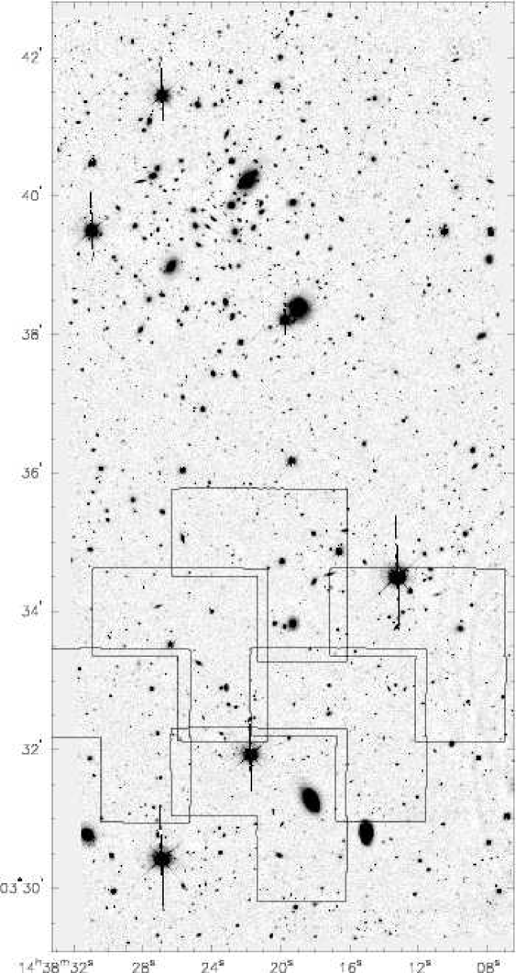
Our analysis concentrates on the same $I$-band image as used in Erben et al. (2000), as this covers most of the area imaged by the HST. We use Chip 3 of a mosaic observation of Abell 1942 taken with the UH8K camera, with a pixel scale of $0\aas@@fstack{\prime\prime}206$. 9 exposures of 1200 s went into the final image, which has a seeing of $0\aas@@fstack{\prime\prime}74$. Unfortunately, a photometric calibration is missing.

2.2 Space-based data

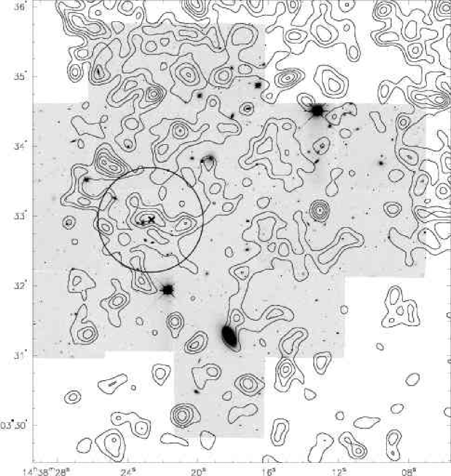
Our HST data is a WFPC2 mosaic (approximately 5$\arcmin\times 4\arcmin$) of six pointings, each consisting of 12 dithered exposures with an exposure time of 400s each, taken between May 20th and June 1st, 2001. The position of the mosaic with respect to the $I$-band image from the CFHT is shown in Fig. 1 The filter employed was F702W.

Figure 1: The outlines of the six HST pointings superposed on the CFHT $I$-band image. The center of Abell 1942 lies in the top half of the CFHT image, the HST mosaic is centered on the dark clump position.

2.2.1 Data reduction

Our reduction of the HST data is based largely on the dither package (Fruchter & Hook 2002) for IRAF. Each of the six pointings was reduced separately. Simultaneous processing of the four individual chips is done automatically by the dither routines. Due to their better signal-to-noise behavior, only the chips of the Wide Field Camera, namely Chips 2, 3, and 4 of WFPC2, were used for the later analysis. The dither pattern of the images allows us to achieve a higher resolution in the coadded image via the drizzle algorithm (Gonzaga et al. 1998).

The steps of the reduction are outlined in the following:

Rough cosmic ray removal:

To find the offsets between the images, they first have to be cleaned of cosmic rays, which would otherwise falsify a cross-correlation. Each frame is cleaned using the precor task. This leaves only objects of a minimal size in the image, which should be stars and galaxies, with little contamination by cosmic rays.

Offset estimation:

As the individual frames are dithered with respect to each other, it is necessary to find their relative offsets. This is done by performing a cross correlation of the cosmic ray cleaned images produced in the previous step.

Median coaddition:

Using the previously determined offsets, the original images are median combined. They are mapped via the drizzle algorithm onto an output grid with pixels of half the original size.

Mask creation:

The median image is mapped back onto the original resolution and offset of the original frames using the blot algorithm, the inverse of drizzle. The original frame is then compared to the median image to identify cosmic rays via the deriv and driz_cr tasks. Thus, for each frame a mask is created identifying cosmic rays. This is combined with a mask identifying defect or possibly problematic pixels, which is supplied with each raw frame.

Offset determination:

For each frame, those pixels that are flagged in the mask are substituted by their value in the blotted image (the transformed median image). These images are then cross-correlated to determine the offsets more precisely. Possible small rotation angles have to be found manually.

Coaddition:

The images are drizzled onto an output grid of half the pixel size (pix-frac = 0.5), i.e. twice the original resolution. The value of each output pixel is obtained via averaging, where pixels which are flagged in the mask image are omitted. The drop-size (i.e. a scaling applie to the input pixels before being mapped) used is 0.6 .

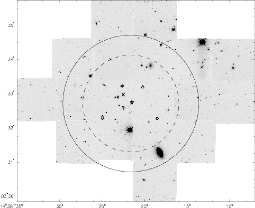
Performing this routine on all of the six pointings, we obtain 18 single-chip images. A mosaic of these is shown in Figure 2.

Figure 2: The HST mosaic with an illustration of the various dark clump centroids cited in the text: the centroid we found in the ground-based data ($\>\star\>$); the original position given by Erben et al. (2000) ($\>+\>$); the peak position in the HST data ($\>\triangle\>$); the center of the X-ray emission as found by ROSAT ($\>*\>$) and by Chandra ($\>\times\>$); the position of the peak found in the 200$\arcsec$ filter scale for the faint ground-based galaxies ($\>\circ\>$); and the galaxy number overdensity of medium-bright HST galaxies ($\>\Diamond\>$). Additionally, we plot a circle of $120\arcsec$ radius around the first position. For our $M_{\rm ap}$ filter function of this radius, the maximal weight is then assigned along the dashed circle. Assuming a typical uncertainty of $1\arcmin$ for centroids found via weak lensing, all cited position are compatible with the dark clump.

2.3 Catalog extraction

For both datasets, we used a similar process to build the object catalogs. Differences in the procedure arise mainly from the small field-of-view and mosaic nature of the HST data.

2.3.1 Preparatory steps

We manually updated the astrometric information of the ground-based image until its bright objects coincide with their positions as given in the USNO-A2 catalog (Monet et al. 1998). This step is not necessary for the lensing analysis of the ground-based image, but provides us with a reference catalog for the astrometric calibration of the HST mosaic.

The HST images are aligned roughly with sky coordinates, but since each chip is read out along a different chip border, the individual images are rotated with respect to each other. To avoid confusion, we first rotate the images of Chips 2 and 4 by $\mp 90^{\circ}$, respectively, such that north is up and east to the left (approximately). This is performed solely as a rearrangement of pixel values to avoid any additional resampling process.

2.3.2 Masking

In order to avoid noise signals and distorted ellipticity measurements, we mask out bright stars and the artefacts they cause (diffraction spikes, blooming, CTE trails, a ripple-like structure at the eastern edge of the $I$-band image, and brightening of the background along columns of the HST chips in two cases). In the HST image, we also mask the bright galaxy in the field.

2.3.3 Source extraction

We used SExtractor (Bertin & Arnouts 1996) to identify objects in the image. SExtractor considers $N$ connected pixels that are at a level $k\cdot\sigma_{\rm sky}$ above the sky background as an object, with $\sigma_{\rm sky}$ being the standard deviation of the background noise. For the CFHT image, we used $N=3$ and $k=1.0$. These are very low thresholds, but since we later want to correlate objects present in both datasets, we strive to obtain a high number density of objects. For the HST images we used $N=3$ and $k=1.5$.

HST: astrometric and photometric calibration

The astrometric calibration plays an important role for a mosaic dataset such as our HST images, as it gives the position of the images with respect to each other. Indeed, the positions on the sky will be used later on in the lensing analysis rather than $x$ and $y$ position on the chip.

For a reference catalog, we had extracted a catalog of bright objects from the astrometrically calibrated ground-based $I$-band image (see Sect. 2.3.1). We match the entries of the reference catalog to objects found in the HST images. This allows the determination of the pointing and the distortion of the image. Objects that are detected both in the $I$-band and the HST image can then be identified by sky coordinates.

The photometric calibration is done based on the relevant keywords of the HST image headers.

2.3.4 Ellipticity measurement

For the objects in the SExtracted catalogs, we measure the ellipticities using a modified version of the imcat software, following the method of Kaiser et al. (1995). We used the half-light radius as measured by SExtractor as the radius of the weight function with which the brightness profile is weighted.

The measured image ellipticity ${\rm\chi}$ is related to the source ellipticity $\mbox{\boldmath${\rm\chi}$\unboldmath}^{(s)}$ by

$$\mbox{\boldmath${\rm\chi}$\unboldmath}=\mbox{\boldmath${\rm\chi}$\unboldmath}^{(s)}+\@tens{P}^{\rm g}\bf{g}+\@tens{P}^{\rm sm}\mbox{\boldmath${\rm q}$\unboldmath}^{\star}\;,$$ (1)

where $\bf{g}$ is the reduced shear induced by a lensing mass which we ultimately want to determine. $\mbox{\boldmath${\rm q}$\unboldmath}^{\star}$ is the stellar anisotropy kernel, i.e. the anisotropy of the PSF for point-like objects. $\@tens{P}^{\rm g}$ and $\@tens{P}^{\rm sm}$ (smear polarizibility tensor) are tensors describing a galaxy’s susceptibility to the two distorting effects. They are also measured from a galaxy’s light distribution (see Bartelmann & Schneider 2001, for a derivation).

2.3.5 Anisotropy correction

To correct for the anisotropy induced by the telescope–detector system, we measure the ellipticities of the stars present in the field; for these eq. (1) simplifies to

$$\mbox{\boldmath${\rm\chi}$\unboldmath}^{\star}=\@tens{P}^{\star\rm sm}\mbox{\boldmath${\rm q}$\unboldmath}^{\star}\;.$$ (2)

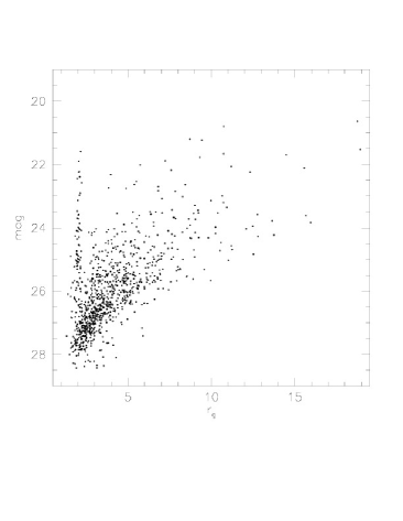
Stars are selected from a magnitude vs. radius plot. We fit a third-order polynomial in chip position $(x,y)$ to the quantity $\left(\frac{\mbox{\boldmath${\rm\chi}$\unboldmath}^{\star}}{0.5\,{\rm tr}(\@tens{P}^{\star\rm sm})}\right)(x,y)$ to estimate $\mbox{\boldmath${\rm q}$\unboldmath}^{\star}(x,y)$.

Thus, we obtain anisotropy-corrected ellipticity measurements:

$$\mbox{\boldmath${\rm\chi}$\unboldmath}^{\rm aniso}=\mbox{\boldmath${\rm\chi}$\unboldmath}-\@tens{P}^{\rm sm}\mbox{\boldmath${\rm q}$\unboldmath}^{\star}\;.$$ (3)

2.3.6 Modification for the HST images

Since the PSF cannot be described analytically across chip-borders, the anisotropy correction for a mosaic has to be applied to the single chips. With the small field of view of the WF chips, we have the added difficulty that for each image, there are only about five stars that could be used for the polynomial fitting, obviously not enough. Since the images were taken consecutively, we can assume that the PSF does not change considerably between the six pointings. We therefore apply an anisotropy correction for each chip based upon all the stars that were found in the six images taken by that chip.

The 18 single-chip catalogs are combined to three catalogs, one for each chip. Because there are still few stars even in these catalogs, the stellar sequence is selected manually. For each catalog, a third-order polynomial is fitted.

The anisotropy correction of the HST images is further discussed in Appendix A.1.

2.3.7 Shear estimation

After the anisotropy correction, the second step in retrieving an estimate of the local shear from ellipticity measurements is the correction for the $\@tens{P}^{\rm g}$ tensor. It is a combination of $\@tens{P}^{\rm sm}$ and the shear polarizibility tensor $\@tens{P}^{\rm sh}$:

$$\@tens{P}^{\rm g}=\@tens{P}^{\rm sh}-\@tens{P}^{\rm sm}(\@tens{P}^{\star\rm sm})^{-1}\@tens{P}^{\star\rm sh}\;,$$ (4)

where the starred quantities are the corresponding tensors as measured on stellar-sized objects. Note that the weight function with which $\@tens{P}^{\star\rm sh}$ and $\@tens{P}^{\star\rm sm}$ are measured should be the same as that used for the respective object.

The basic assumption of weak lensing studies is that the average source ellipticities vanish, i.e. $\langle\mbox{\boldmath${\rm\chi}$\unboldmath}^{(s)}\rangle=0$. We also assume that $\langle(\@tens{P}^{\rm g})^{-1}\mbox{\boldmath${\rm\chi}$\unboldmath}^{s}\rangle=0$, so by averaging eq. (1) we obtain:

$${\bf g}=\langle(\@tens{P}^{\rm g})^{-1}\mbox{\boldmath${\rm\chi}$\unboldmath}^{\rm aniso}\rangle\;.$$ (5)

Thus the expectation value of the quantity $(\@tens{P}^{\rm g})^{-1}\mbox{\boldmath${\rm\chi}$\unboldmath}^{\rm aniso}$ is the reduced shear ${\bf g}$ at the respective point.

$\@tens{P}^{\rm g}$ is an almost diagonal tensor with similar elements on the diagonal. In fact, in the absence of a weight function and a PSF its elements would be: $P^{\rm g}_{11}=P^{\rm g}_{22}=2$ , $P^{\rm g}_{12}=P^{\rm g}_{21}=0$. We can therefore approximate the tensor $\@tens{P}^{\rm g}$ by a scalar quantity:

$$P^{\rm g}_{s}\;=\;\frac{1}{2}\,{\rm tr}(\@tens{P}^{\rm g})\;.$$ (6)

It has been shown that while the full $\@tens{P}^{\rm g}$ tensor can overestimate the shear, this approximation is more conservative and will only underestimate the true shear (Erben et al. 2001).

We therefore use a variant of eq. (5) as our estimate of the local shear at each galaxy’s position:

$$\mbox{\boldmath${\rm\varepsilon}$\unboldmath}=\frac{\mbox{\boldmath${\rm\chi}$\unboldmath}^{\rm aniso}}{P^{\rm g}_{s}}\;.$$ (7)

At this point, we reject those objects from the catalog that have a radius equal to or smaller than the stellar locus, are saturated stars, or have a final ellipticity of $|\mbox{\boldmath${\rm\varepsilon}$\unboldmath}|>1$.

2.3.8 Rotation of ellipticities

The ellipticities were measured with respect to the $x$-axis of each image, which for all images runs approximately along the east axis. However, the lensing analyses are done in sky coordinates. We therefore need to transform the ellipticity measurements so that their position angle is measured relative to the right ascension axis. This is done with the transformation

$$\mbox{\boldmath${\rm\varepsilon}$\unboldmath}\;\rightarrow\;\mbox{\boldmath${\rm\varepsilon}$\unboldmath}\,\mathrm{e}^{2\mathrm{i}\varphi}$$

where $\varphi$ is the angle of rotation of the image.

After this step, the 18 single-image catalogs of the HST data are merged into one catalog.

2.3.9 Weighting

To describe the reliability of its shape measurement, we want to assign a weight to each galaxy, based on its noise properties. Since our shear estimates are gained from averages over ellipticities, a good weight estimate is

$$w_{i}\;\propto\;\frac{1}{\sigma_{i}^{2}}\;.$$ (8)

where $\sigma_{i}$ is the (two-dimensional) dispersion of image ellipticities in the ensemble over which is averaged. For intrinsic ellipticities, $\sigma_{\varepsilon}\approx 0.3-0.4$ (measured from data). Measurement errors cause $\sigma_{i}$ to be higher than this. We follow the weighting scheme of Erben et al. (2001), and select as the ensemble to average over the 20 closest neighbors of the respective galaxy in the parameter space spanned by half-light radius $r_{g}$ and magnitude $m$.

2.3.10 Final cuts

After the weighting, we remove objects with $|\varepsilon|>0.8$. Such objects would dominate the shear signal, but these are also the objects that are most afflicted by noise in the $P^{g}$ tensor. Additionally, we use only objects for which $P^{g}>0.3$. This leaves about 2000 objects in both catalogs, which corresponds to 20 galaxies/arcmin² for the $I$-band image and 65 galaxies/arcmin² for the HST image.

3 Weak lensing methods

Weak lensing analyses are based on using estimates of the local shear ${\rm\gamma}$ to reconstruct information on the convergence $\kappa$, which is a dimensionless measure of the surface mass density. In the weak lensing regime, $\kappa\ll 1$, so that $\langle\mbox{\boldmath${\rm\varepsilon}$\unboldmath}\rangle={\bf g}=\mbox{\boldmath${\rm\gamma}$\unboldmath}/(1-\kappa)\approx\mbox{\boldmath${\rm\gamma}$\unboldmath}$.

3.1 Mass reconstruction

Both the shear ${\rm\gamma}$ and the convergence $\kappa$ are linear combinations of second derivatives of the lensing potential, so that it is possible to express $\kappa$ as an integral over ${\rm\gamma}$ via the Kaiser–Squires Inversion (Kaiser & Squires 1993). This method is usually not applied directly, as the shot noise introduced by summing over individual galaxies (shear measurements) produces infinite noise. This can be avoided by first smoothing the shear measurements; however, such a smoothing scale introduces correlated errors. Another problem arises from the limited field-of-view of any observations. Seitz & Schneider (2001) express this as a von Neumann boundary problem, leading to the so-called finite–field inversion. We rely on this method for mass reconstructions throughout the paper.

3.2 Mass-aperture statistics

The mass-aperture, or $M_{\rm ap}$, Statistics, developed by Schneider (1996), provides a method with defined noise properties to identify mass concentrations. It is based upon the relation

$$M_{\rm ap}(\@vec{\theta}_{0})=\!\int_{{\rm I\mathchoice{\kern-1.99168pt}{\kern-1.99168pt}{\kern-1.84941pt}{\kern-1.42262pt}R}^{2}}\!{\rm d}^{2}\theta\;\kappa(\@vec{\theta}_{0}+\@vec{\theta})\>w(|\@vec{\theta}|)=\!\int_{{\rm I\mathchoice{\kern-1.99168pt}{\kern-1.99168pt}{\kern-1.84941pt}{\kern-1.42262pt}R}^{2}}\!{\rm d}^{2}\vartheta\>\gamma_{\rm t}(\@vec{\theta}_{0};\@vec{\vartheta})\,Q(|\@vec{\vartheta}|)\;.$$ (9)

The aperture mass $M_{\rm ap}(\@vec{\theta}_{0})$ presents a measure of the average convergence, mulitplied with a filter function $w$, around a position $\@vec{\theta}_{0}$ in the lens plane. If $w(|\@vec{\theta}|)$ is a compensated filter, $M_{\rm ap}$ avoids the mass sheet degeneracy. The right side of eq. (9) expresses $M_{\rm ap}$ in terms of the tangential shear $\gamma_{\rm t}$ at the position $\@vec{\theta}_{0}+\@vec{\vartheta}$ with respect to $\@vec{\theta}_{0}$:

$$\gamma_{\rm t}(\@vec{\theta}_{0};\@vec{\vartheta})=-\mathcal{R}e\left(\mbox{\boldmath${\rm\gamma}$\unboldmath}(\@vec{\theta}_{0}+\@vec{\vartheta})\mathrm{e}^{-2\mathrm{i}\phi}\right)\;,$$ (10)

where $\phi$ is the polar angle of the vector $\@vec{\vartheta}$. The weight function $Q$ is determined in terms of $w$.

Eq. (9) is intuitively clear: a lens most often deforms images so they align tangentially to the center of mass. An average over the tangential components of galaxy ellipticities must therefore be a measure of the surface mass. With this interpretation, $M_{\rm ap}$ is a useful quantity in its own right even if the weak lensing assumption, $\mbox{\boldmath${\rm\gamma}$\unboldmath}=\langle\mbox{\boldmath${\rm\varepsilon}$\unboldmath}\rangle$, breaks down or if part of the weight function lies outside the field.

The imaginary shear component is the cross component:

$$\gamma_{\times}(\@vec{\theta}_{0};\@vec{\vartheta})=-\mathcal{I}m\left(\mbox{\boldmath${\rm\gamma}$\unboldmath}(\@vec{\theta}_{0}+\@vec{\vartheta})\mathrm{e}^{-2\mathrm{i}\phi}\right)\;.$$ (11)

Substituting it for the tangential shear in eq. (9) yields $M_{\rm ap}^{\times}$ whose expectation value vanishes. Evaluating it analogous to $M_{\rm ap}$ can thus be used as a method to check the quality of the dataset.

3.2.1 Application to real data

• In order to apply the weight function $Q$ to finite data fields, a cut-off radius $\theta_{\rm out}$ should be used, beyond which the filter function vanishes. Otherwise, the area of integration is not well sampled by galaxy images. A compensated filter $w(|\@vec{\vartheta}|)$, for which $w(|\@vec{\vartheta}|)\equiv 0$ for $|\@vec{\vartheta}|>\theta_{\rm out}$ yields a weight function $Q(|\@vec{\vartheta}|)$ which vanishes beyond the same cut-off radius. We use filter and weight function as introduced in Schneider et al. (1998), with $l=1$.

  

  Figure 3: The filter function $w$ (solid line) we used and its corresponding weight function $Q$ (dashed line) shown in units of $\theta_{\rm out}$.

• We can sample the shear field only at discrete points, namely those where there is a measured galaxy image. In the weak lensing regime, the image ellipticity is on average a direct measure of the shear, so that we can use the tangential ellipticity $\varepsilon_{\rm t}$ as an estimate for the tangential shear $\gamma_{\rm t}$ ($\varepsilon_{\rm t}$ defined analogously to $\gamma_{\rm t}$).

We thus estimate $M_{\rm ap}$ by using

$$M_{\rm ap}(\@vec{\theta}_{0};\theta_{\rm out})\;=\;\frac{\pi\theta_{\rm out}^{2}}{N}\sum\limits_{i}\varepsilon_{\rm t}(\@vec{\theta}_{i})\,Q(|\@vec{\theta}_{i}-\@vec{\theta}_{0}|)\;,$$ (12)

where $i$ runs over all $N$ galaxies within a radius $\theta_{\rm out}$ from the point $\@vec{\theta}_{0}$.

With the weighting scheme introduced in eq. (8), this becomes:

$$M_{\rm ap}(\@vec{\theta}_{0};\theta_{\rm out})\;=\;\pi\theta_{\rm out}^{2}\,\frac{\sum_{i}\varepsilon_{\rm t}(\@vec{\theta}_{i})\,\sigma_{i}^{-2}\,Q(|\@vec{\theta}_{i}-\@vec{\theta}_{0}|)}{\sum_{i}\sigma_{i}^{-2}}\;.$$ (13)

3.2.2 Significances

Any $M_{\rm ap}$ value is incomplete without an estimate of its significance, i.e. how it compares to the typical noise level of the $M_{\rm ap}$ estimator. The signal-to-noise ratio is given by

$$\frac{S}{N}=\frac{M_{\rm ap}}{\sigma_{M_{\rm ap}}}=\frac{M_{\rm ap}}{\sqrt{\langle M_{\rm ap}^{2}\rangle-\langle M_{\rm ap}\rangle^{2}}}\;,$$ (14)

where the denominator should represent the case of no lensing. The expectation value $\langle M_{\rm ap}\rangle$ of $M_{\rm ap}$ then vanishes since the galaxies are oriented completely randomly and thus $\langle\varepsilon_{\rm t}\rangle$, the expectation value of tangential ellipticities, vanishes. In the case of a non-weighted $M_{\rm ap}$ estimator, we obtain:

$$\langle M_{\rm ap}^{2}\rangle\;=\;\frac{\left(\pi\theta_{\rm out}^{2}\right)^{2}}{N^{2}}\,\sum\limits_{i}\,\langle\varepsilon_{\rm t}^{2}(\@vec{\theta_{i}})\rangle\,Q^{2}(|\@vec{\theta}_{i}-\@vec{\theta}_{0}|)\;.$$ (15)

In the case of no lensing, $\langle\varepsilon_{{\rm t},i}^{2}\rangle$ is the one-dimensional variance of the intrinsic ellipticities:

$$\langle\varepsilon_{{\rm t},i}^{2}\rangle=\frac{1}{2}\,\sigma_{\varepsilon}^{2}$$ (16)

and the signal-to-noise ratio becomes:

$$\frac{S}{N}\;=\;\frac{\sqrt{2}}{\sigma_{\varepsilon}}\>\frac{\sum_{i}\varepsilon_{\rm t}(\@vec{\theta}_{i})\,Q(|\@vec{\theta}_{i}-\@vec{\theta}_{0}|)}{\sqrt{\sum_{i}Q^{2}(|\@vec{\theta}_{i}-\@vec{\theta}_{0}|)}}\;.$$ (17)

For the weighted estimator, one faces the problem that the weights $1/\sigma_{i}^{2}$ are in general not completely independent of the tangential ellipticity $\varepsilon_{t,i}$. We assign weights to galaxy images by considering the variance of ellipticities of an ensemble of galaxy images with similar noise properties. But in general, large ellipticities are often noise-afflicted, so that they are assigned a lower weight. The expression for $\langle M_{\rm ap}^{2}\rangle$ then cannot be simplified ad hoc:

$$\langle M_{\rm ap}^{2}\rangle\;=\;(\pi\theta_{\rm out}^{2})^{2}\,\left\langle\frac{\sum_{i,j}\varepsilon_{{\rm t},i}\varepsilon_{{\rm t},j}\,\sigma_{i}^{-2}\sigma_{j}^{-2}\,Q_{i}Q_{j}}{\sum_{i,j}\sigma_{i}^{-2}\sigma_{j}^{-2}}\right\rangle\;.$$ (18)

The significance of a detection is related to the probability that the observed alignment of tangential ellipticities can be mimicked by a random distribution of galaxy ellipticities. A commonly used possibility to determine the significance is therefore to randomize the position angles of the galaxy images and calculate $M_{\rm ap}$ of these. This is repeated $N_{\rm rand}$ times.

With this in mind, we reconsider eq. (18). Such randomizations represent a possible ensemble average, which we denote by $\langle\ldots\rangle_{\phi}$. For each realization, the ellipticity modulus remains the same, only the orientation changes. In this case, the weights also remain the same and we can simplify the expression:

$$\langle M_{\rm ap}^{2}\rangle_{\phi}=\left(\pi\theta_{\rm out}^{2}\right)^{2}\frac{\sum_{i,j}\frac{\langle\varepsilon_{{\rm t},i}\varepsilon_{{\rm t},j}\rangle_{\phi}}{\sigma_{i}^{2}\sigma_{j}^{2}}\;Q_{i}Q_{j}}{\left(\sum_{i}\frac{1}{\sigma_{i}^{2}}\right)^{2}}=\frac{(\pi\theta_{\rm out}^{2})^{2}}{2}\;\frac{\sum_{i}\frac{|\mbox{\boldmath${\rm\varepsilon}$\unboldmath}_{i}|^{2}}{\sigma_{i}^{2}}\>Q_{i}^{2}}{\left(\sum_{i}\frac{1}{\sigma_{i}^{2}}\right)^{2}}$$

since, as the ellipticity modulus is fixed,

$$\langle\varepsilon_{{\rm t},i}\varepsilon_{{\rm t},j}\rangle_{\phi}=\frac{|\mbox{\boldmath${\rm\varepsilon}$\unboldmath}_{i}|^{2}}{2}\>\delta_{ij}\;.$$

The signal-to-noise ratio for the weighted estimator is therefore:

$$\frac{S}{N}\;=\;\sqrt{2}\>\sum_{i}\frac{\varepsilon_{\rm t}(\@vec{\theta}_{i})\>\sigma_{i}^{-2}\,Q(|\@vec{\theta}_{i}-\@vec{\theta}_{0}|)}{\sqrt{\sum_{i}|\mbox{\boldmath${\rm\varepsilon}$\unboldmath}_{i}|^{2}\,\sigma_{i}^{-2}\>Q^{2}(|\@vec{\theta}_{i}-\@vec{\theta}_{0}|)}}\;.$$ (19)

To check the validity of the assumptions we made, we compared results from randomizations and this analytic formula and found them to be equivalent.

4 Re-analysis of the CFHT data

In Table 1, we summarize the differences between the analyses of Erben et al. (2000) and this work.

Table 1: Summary of the differences of the object catalogs used for the lensing analyses of Erben et al. (2000) and this work. The brightness key refers to the magnitude bins used to split the sample (note that the magnitudes are not calibrated).

	Erben et al. (2000)	this work
masking	$-$	$\surd$
source extraction	$6\,{\rm px}\geq 1.0\sigma$	$3\,{\rm px}\geq 1.0\sigma$
weighting	$-$	$\surd$
$|\mbox{\boldmath${\rm\varepsilon}$\unboldmath}|$	$\leq 1.0$	$\leq 0.8$
brightness	$m\gtrsim 23$	$all$
		$m\geq 23.67$
		$22.54<m<23.67$
		$m\leq 22.54$

4.1 Mass reconstruction

Figure 4: Mass reconstruction of the CFHT $I$-band image according to Seitz & Schneider (2001). Solid (dashed) lines give positive (negative) $\kappa$ contours, starting at $\pm 0.02$ and in-(de-)creasing in 0.01 intervals. The smoothing scale is 60″.

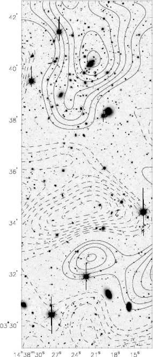
In order to apply the finite-field inversion (Sect. 3.1), we further cut the $I$-band image to avoid the ripple-like reflection artefact at the eastern edge altogether. This narrows the available field, but avoids problems at the boundaries. A resulting mass reconstruction is shown in Fig. 4.

Abell 1942 shows up prominently in the top half of the field, with the peak of the mass map centered approximately on the cD galaxy. In the lower half of the image, there is a second, albeit lower peak at the same position as detected in Erben et al. (2000). Relative to the peak $\kappa$ of A1942, our dark clump signal is slightly larger than given by Erben et al. (2000). However, north of the dark clump, there is a “hole” - a region of significantly negative $\kappa$ values. Although this is a somewhat disconcerting result, it must be stressed that $\kappa$ is underestimated in the whole field due to the mass sheet degeneracy and the cluster in the field (two of the three field boundaries close to the cluster and well within its extent display nearly vanishing $\kappa$ values). Unfortunately, the original analysis of Erben et al. (2000) only investigates regions of positive $\kappa$, so that this result cannot be compared.

4.2 $M_{\rm ap}$ analysis

4.2.1 Complete sample

Figure 5: Results of a weighted $M_{\rm ap}$ analysis of the $I$-band data. Shown are positive (negative) S/N contours as solid (dashed) lines starting at $\pm$ 2.0$\sigma$ in 0.5$\sigma$ intervals. The filter scales from left to right are 80$\arcsec$, 120$\arcsec$, 160$\arcsec$, and 200$\arcsec$. The dark clump signal shows up strongest in the 120$\arcsec$ filter, with a peak significance of 4.9$\sigma$.

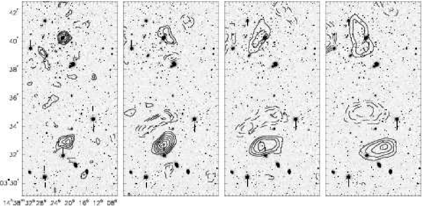
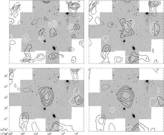
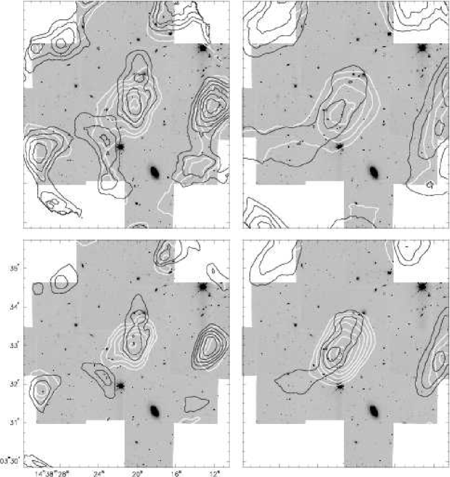
We perform the $M_{\rm ap}$ analysis as described in Sect. 3.2 and evaluate the $M_{\rm ap}$ statistic on a grid with grid spacings of 2$\arcsec$. The result is shown in Fig. 5. The dark clump signal is seen significantly at all filter scales, but it is particularly strong for the 120$\arcsec$ filter, where it reaches a peak significance of 5$\sigma$. In the other filters, the significance is at the 3.5$\sigma$ level, as in Erben et al. (2000).

Abell 1942 is detected only weakly for large filter scales, a result that is consistent with Erben et al. (2000). The mass reconstruction from the previous paragraph demonstrates why the dark clump reaches a much higher $M_{\rm ap}$ significance than the cluster: at the dark clump position, the negative part of the filter function (Fig. 3) is evaluated largely at the position of the hole, thereby boosting the signal. The same in reverse is true for the hole itself: its significance is boosted by its proximity to the Dark Clump. Yet its significance remains lower than that of the dark clump.

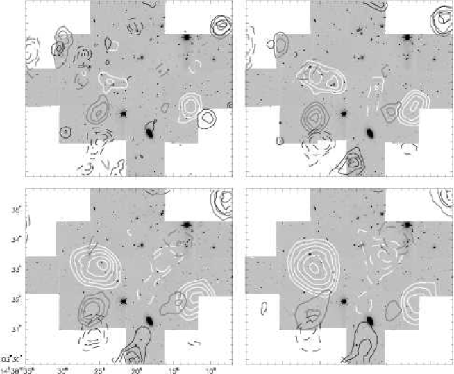
4.2.2 Rough redshift dependence

Figure 6: The same as the previous figure (Fig. 5), but with the galaxies divided into three magnitude bins and only positive contours. White contours correspond to the brightest galaxies, gray contours to those of medium brightness, and black contours to the faintest.

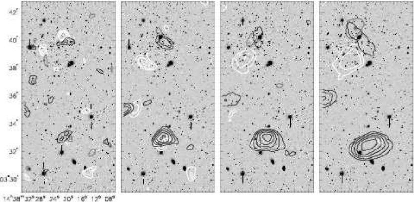
On average, the more distant a galaxy, the fainter it is. By introducing magnitude cuts we split the galaxy sample into three parts of about 660 galaxies each with different mean redshift. This is a very crude redshift distinction, but should reveal any trend of lens strength with redshift.

The results of this analysis are shown in Fig. 6. We see that the dark clump signal stems mostly from faint galaxies, which supports the notion that this is a high-redshift object. However, these are also those objects that are most subject to noise effects.

At the 120$\arcsec$ filter scale, there is also a 3$\sigma$ contribution from bright galaxies. Assuming that the lensing mass is indeed a high redshift object, these bright galaxies are unlikely to be at higher redshifts. Thus, this is probably not a lensing signal. Yet, this “contamination” can explain the high signal-to-noise ratio we see at this filter scale.

For Abell 1942, there is a strong signal at the smallest filter scale, centered on the cD galaxy which exhibits a strong lensing arc. It may well be that at these radii we are not in the weak lensing regime any more and the tangential alignment is already rather distinct. In the other filter radii, there is no particularly strong signal. This might be due to the generic weight function which is not adapted to the NFW profile.

Our plot does not show the negative $M_{\rm ap}$ contours to avoid overcrowding. Unlike to the dark clump, all three magnitude bins contribute to the “hole”.

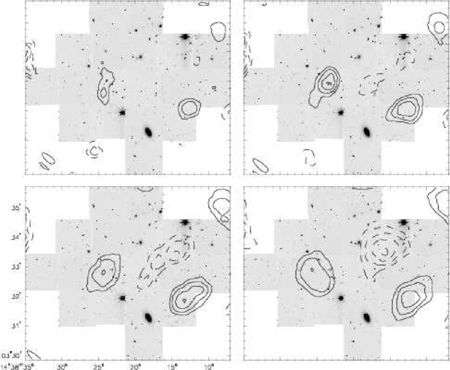
4.2.3 $M_{\rm ap}$ cross component

In Sect. 3.2, we argued that $M_{\rm ap}^{\times}$, i.e. $M_{\rm ap}$ calculated with the cross component of the shear instead of the tangential one, must vanish. By checking the validity of this assumption in the dataset, we can identify possible problems.

Figure 7: Results of a $M_{\rm ap}^{\times}$ analysis of the $I$-band image. Shown are both positive (white) and negative (black) contours, starting at $\pm 2\sigma$ in 0.5$\sigma$ increments, for filter scales of 80$\arcsec$, 100$\arcsec$, 160$\arcsec$, and 200$\arcsec$ (left to right).

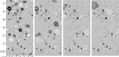
The results are shown in Fig. 7. Particularly at small filter scales, there are some positive and negative peaks with significances ${\scriptstyle\gtrsim}|3\sigma|$ (negative values are indicated by negative signal-to-noise ratios). However, most of the peaks are at the edge of the field, where a part of the weight function lies outside the field. While (the real part of) $M_{\rm ap}$ retains its justification at these places as being simply a measure of the tangential alignment, we can no longer assume that $M_{\rm ap}^{\times}$ vanishes.

There is no peak with a significance larger than 2$\sigma$ in the vicinity of the dark clump, so the detection passes this test well.

4.3 Radial profile

Figure 8: The mean tangential ellipticity $\langle\mbox{\boldmath${\rm\varepsilon}$\unboldmath}_{t}\rangle$ relative to the position of the Dark Clump as a function of distance from it (from the ground-based data). Each point corresponds to the mean of a 20$\arcsec$ wide bin, where filled circles denote the complete sample, crosses the faint galaxies, triangles the medium bright ones, and squares the bright galaxies. The error bars represent the standard deviation of $\langle\mbox{\boldmath${\rm\varepsilon}$\unboldmath}_{t}\rangle$ estimated from randomization of the position angles of the galaxies. Note that the first bin is very sensitive to the choice of centroid - its deviation from the shear profile in the latter bins is thus not problematic.

Despite several differences to the lensing analysis of Erben et al. (2000), the $M_{\rm ap}$ results agree at least qualitatively. We are curious whether we can also reproduce the radial dependence of the mean tangential ellipticity shown in Fig. 9 of Erben et al. (2000).

We determine the position of the dark clump from the $M_{\rm ap}$ peak at the 120$\arcsec$ filter scale, where the signal is strongest. We find it to be $\alpha=14^{\rm h}\,38^{\rm m}\,21.6^{\rm s},\>\delta=3^{\circ}\,32\arcmin\,43\aas@@fstack{\prime\prime}$ , which is at a distance of $18\aas@@fstack{\prime\prime}6$ from the position given by Erben et al. (2000), and thus just at the 1$\sigma$ level they give for the uncertainty of the centroid’s position.

The tangential ellipticity relative to this position is calculated for each galaxy within 200$\arcsec$. They are then binned according to their distance from the dark clump and the weighted mean is calculated for each bin. To estimate the standard deviation, we randomize the position angles of these galaxies 1000 times and calculate the mean tangential ellipticity each time, thus gaining an estimate for the standard deviation. This analysis is done for the complete galaxy sample as well as the three samples split according to brightness. The results of it are shown in Fig. 8.

Particularly for the faintest galaxies, we find positive values out to 120$\arcsec$. This agrees well with the strong shear signal seen for these galaxies. We can also identify the cause of the signal seen for bright galaxies at the 120$\arcsec$ filter scale: the two significantly positive bins at 90$\arcsec$ and 110$\arcsec$ (the filter function employed assigns the highest weight around a radius $\theta_{\rm out}/\sqrt{2}$). For the medium bright galaxies $\langle\mbox{\boldmath${\rm\varepsilon}$\unboldmath}_{t}\rangle$ is largely consistent with zero.

Compared to Erben et al. (2000), who measure $\langle\mbox{\boldmath${\rm\varepsilon}$\unboldmath}_{t}\rangle\approx 0.06$ at 100$\arcsec$, we find a higher value ($\approx 0.1$). On the other hand, we find positive values only out to 120$\arcsec$ rather than 150$\arcsec$. And since the centroid positions do not coincide, the inner two bins are not comparable. Yet, we can also be confident that the signal is not caused just by a few galaxies.

Table 2: Overview of the $M_{\rm ap}$ values and signal-to-noise ratios of the peaks found in the analyses of the CFHT data. We also give the number of galaxies located in the aperture ($N$), and the (weighted) average galaxy ellipticity dispersion $\sigma_{\varepsilon}$, as well as the offset to the assumed centroid position, measured in the sky coordinate system. In two cases, there was no $M_{\rm ap}$ peak in the vicinity of the dark clump - we then quote the values at the reference position (in italics).

	$\theta_{\rm out}$	N	$\sigma_{\varepsilon}$	$\Delta\alpha[\arcsec]$	$\Delta\delta[\arcsec]$	$M_{\rm ap}$	SNR
$|\mbox{\boldmath${\rm\varepsilon}$\unboldmath}|<0.8$,	80$\arcsec$	113	0.34	28	16	0.096	3.7
weighted,	120$\arcsec$	268	0.34	0	0	0.078	5.1
all galaxies	160$\arcsec$	468	0.35	$-16$	$-2$	0.046	3.7
	200$\arcsec$	648	0.34	58	$-12$	0.034	3.5
$|\mbox{\boldmath${\rm\varepsilon}$\unboldmath}|<0.8$,	80$\arcsec$	54	0.41	22	26	0.120	2.7
weighted,	120$\arcsec$	110	0.39	4	4	0.109	4.1
$m>23.67$	160$\arcsec$	167	0.38	36	18	0.092	4.3
	200$\arcsec$	241	0.39	40	$-22$	0.088	4.5
$|\mbox{\boldmath${\rm\varepsilon}$\unboldmath}|<0.8$,	80$\arcsec$	33	0.34	40	8	0.118	2.6
weighted,	120$\arcsec$	86	0.35	6	$-18$	0.058	2.0
$22.54<m<23.67$	160$\arcsec$	159	0.36	$-26$	2	0.031	1.5
	200$\arcsec$	222	0.34	$-$	$-$	$-$0.003	$-$0.1
$|\mbox{\boldmath${\rm\varepsilon}$\unboldmath}|<0.8$,	80$\arcsec$	35	0.29	38	4	0.084	2.2
weighted,	120$\arcsec$	74	0.29	16	0	0.075	3.5
$m<22.54$	160$\arcsec$	126	0.30	$-14$	$-20$	0.046	2.3
	200$\arcsec$	170	0.30	$-48$	34	0.026	1.6

4.4 Summary

We have successfully confirmed the weak lensing signal seen in two sets of CFHT observations (our re-analysis of the $V$-band data are not shown here but agree well with Erben et al. (2000)). We show that the alignment signal comes from faint galaxies, which supports the hypothesis that it is caused by a lensing mass at high redshifts. One must keep in mind, however, that these are also those objects most affected by noise.

With several variations of the catalog that enters the $M_{\rm ap}$ analysis, we tested that the detection of the dark clump is resistant against these and consistently recovered at all filter scales. It reaches a peak significance of about 5$\sigma$, although this signal is contaminated by a tangential alignment of bright objects, which is unlikely to be a lensing effect.

5 Analysis of the HST data

The HST catalog extends to fainter and thus more distant galaxies than the ground-based catalog. If the alignment signal found in the ground-based data does indeed stem from a mass concentration, its lens strength should increase with source redshift. Additionally, since the HST is space-based and thus not afflicted by atmospheric seeing, its ellipticity measurements are more reliable than those from ground-based telescopes. If the ground-based signal is not just a noise peak, the signal should therefore be even stronger in the HST images.

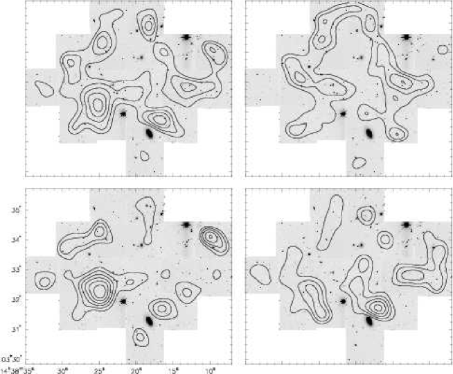
5.1 Mass reconstruction

Figure 9: The mass density map of the inner region of the HST image reconstructed according to the method given in Seitz & Schneider (2001). Shown are $\kappa$ contours starting at $\pm 0.02$ and in-/decreasing in 0.01 decrements. The smoothing length is $30\arcsec$.

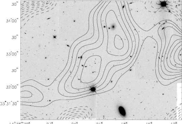
Fig. 9 shows the results of a mass reconstruction of the inner rectangle of the HST data field. The dark clump shows up prominently, slightly westward of the position found in the ground-based analyisis.

5.2 $M_{\rm ap}$ analysis

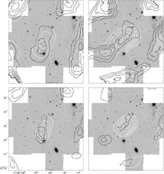
The results of the weighted $M_{\rm ap}$ analysis of the complete catalog is shown in Fig. 10 and summarized in Table 3. Indeed, we find a peak at approximately the same position as in the ground-based images in the 120$\arcsec$ filter, but with only 2.9$\sigma$ significance it is considerably weaker. At the smallest filter scale used ($80\arcsec$), this peak diminishes and dissolves into two peaks.

Figure 10: Results of the $M_{\rm ap}$ analysis of the complete catalog from the HST images. The filter scales are 80$\arcsec$, 100$\arcsec$, 120$\arcsec$, and 140$\arcsec$ (from top left to lower right). The contours start at 1.5$\sigma$ and increase in 0.5$\sigma$ increments.

Just as for the ground-based data, we split the catalog into three bins according to brightness to probe the redshift dependence of the lens strength. With cuts at $m=25.46$ and $m=26.43$, the three samples contain approximately equal numbers of galaxies. The respective $M_{\rm ap}$ analyses are shown in Fig. 11.

Figure 11: The same as the previous figure (Fig. 10), but with the galaxies divided into three bins. White contours correspond to the brightest galaxies, gray contours to those of medium brightness, and black contours to the faintest. The contours start at 1.5$\sigma$ and increase in 0.5$\sigma$ increments.

The alignment signal is carried by the galaxies in the bright and in the faint bin, but there is a lack of signal in the medium-bright bin. The galaxies that were detected in the ground-based image should be mostly contained in the HST’s bright bin. Although the $M_{\rm ap}$ values differ by a factor of about 2, the measurement in the bright bin therefore confirms that there is tangential alignment around the dark clump candidate. However, the lack of alignment in the medium bin is difficult to explain with the lensing hypothesis.

5.3 $M_{\rm ap}$ cross component

Figure 12: The $M_{\rm ap}^{\times}$ analysis of the HST data. Shown are both positive (solid) and negative (dashed) contours, starting at $\pm 1.5\sigma$ in 0.5$\sigma$ increments, for filter scales of 80$\arcsec$, 100$\arcsec$, 120$\arcsec$, and 140$\arcsec$ (upper left to lower right).

Figure 13: The same as Fig. 12, but with the galaxies split into three samples according to brightness. The color coding is identical to that of Fig. 11. The contours start at $\pm 1.5\sigma$ and in-/decrease in 0.5$\sigma$ increments.

Table 3: Overview of the $M_{\rm ap}$ values and signal-to-noise ratios of the peaks found in the analyses of the HST data. We also give the number of galaxies located in the aperture ($N$), and the (weighted) average galaxy ellipticity $\sigma_{\varepsilon}$, as well as the offset to the assumed centroid position, measured in the sky coordinate system. For the small filter scales ($60\arcsec$ and $80\arcsec$), there were often more than one peak in the vicinity of the dark clump position. For the medium bright bin, there is no peak close to the dark clump in the largest two filter scales - we then quote the values at the reference position (in italics).

	$\theta_{\rm out}$	N	$\sigma_{\varepsilon}$	$\Delta\alpha[\arcsec]$	$\Delta\delta[\arcsec]$	$M_{\rm ap}$	SNR
$|\mbox{\boldmath${\rm\varepsilon}$\unboldmath}|<0.8$,	80$\arcsec$	352	0.39	34	32	0.037	2.2
$P^{\rm g}_{s}>0.3$,		410	0.38	$-42$	$-52$	0.033	2.3
weighted,	100$\arcsec$	560	0.39	20	26	0.030	2.2
all galaxies	120$\arcsec$	907	0.39	0	0	0.025	2.4
	140$\arcsec$	1188	0.38	$-22$	6	0.022	2.5
$|\mbox{\boldmath${\rm\varepsilon}$\unboldmath}|<0.8$,	80$\arcsec$	138	0.40	32	$-32$	0.060	2.1
$P^{\rm g}_{s}>0.3$,	100$\arcsec$	212	0.41	0	$-18$	0.060	2.7
weighted,	120$\arcsec$	314	0.42	$-12$	$-10$	0.063	3.3
$m>26.5$	140$\arcsec$	392	0.42	$-12$	12	0.060	3.5
$|\mbox{\boldmath${\rm\varepsilon}$\unboldmath}|<0.8$,	80$\arcsec$	126	0.40	$-$	$-$	$-$0.034	$-$1.3
$P^{\rm g}_{s}>0.3$,	100$\arcsec$	204	0.40	$-$	$-$	$-$0.032	$-$1.5
weighted,	120$\arcsec$	294	0.39	$-$	$-$	$-$0.014	$-$0.7
$25.5<m<26.5$	140$\arcsec$	374	0.40	$-$	$-$	$-$0.008	$-$0.5
$|\mbox{\boldmath${\rm\varepsilon}$\unboldmath}|<0.8$,	80$\arcsec$	134	0.36	18	34	0.068	2.8
$P^{\rm g}_{s}>0.3$,	100$\arcsec$	220	0.36	4	16	0.045	2.4
weighted,	120$\arcsec$	309	0.35	0	0	0.031	1.9
$m<25.5$	140$\arcsec$	402	0.35	$-$	$-$	0.009	0.7

As described in Appendix A.1, it is difficult to judge the quality of the anisotropy correction of the HST data. A faulty anisotropy correction is likely to cause a non-vanishing $M_{\rm ap}^{\times}$ component. Also the CTE problem of the camera might do so. We therefore calculate $M_{\rm ap}$ with the shear cross component instead of the tangential component; the result of this analysis is shown in Fig. 12.

Indeed, there is a 3$\sigma$ peak roughly coincident with the group of galaxies close to the dark clump, and one close to the border of the image. For the latter one, a large part of the aperture is evaluated outside of the field, so that $M_{\rm ap}^{\times}$ is not necessarily expected to vanish in this case. This argument applies only weakly to the first one, which is affected only by masks of stars.

The stellar anisotropy increases with distance from the center of the chips, cf. Fig. 21. At the edges of the chips we also expect the largest deviations of the fit from the actual values. Therefore, the quality of the anisotropy correction should decrease with increasing distance from the chip center. To test this effect, we reject those objects which are more than 700 pixels from the center of their chip (343 objects) and redo the $M_{\rm ap}^{\times}$ analysis. The result differs only very little from the previous one.

We also calculate the $M_{\rm ap}$ cross component for the three brightness bins, Fig. 13. We find that the $M_{\rm ap}^{\times}$ peaks are caused solely by the bright galaxies. If they were caused by an insufficient anisotropy correction, we would expect these peaks to show up for all three bins. Additionally, as the brightest objects are generally also the largest, the effect of the anisotropy correction is smallest for these.

These results indicate that the $M_{\rm ap}^{\times}$ peaks are unlikely to be caused by a poor anisotropy correction. Rather, they seem to be caused by an intrinsic alignment of some of the bright galaxies.

5.4 Radial profile

Figure 14: The mean tangential ellipticity $\langle\varepsilon_{\rm t}\rangle$ to the position of the dark clump (determined from the $M_{\rm ap}$ analysis of the HST data) as a function of distance from it. Each point corresponds to the mean of a 20$\arcsec$ bin, where filled circles denote the complete sample, crosses the faint galaxies, triangles the medium bright ones, and squares the bright galaxies. The error bars represent the standard deviation of $\langle\varepsilon_{\rm t}\rangle$ estimated from randomization of the position angles of the galaxies.

Figure 15: Same as Fig. 14, but with the distance measured relative to the position of the dark clump (as measured in the ground-based data).

Just as described in Sect 4.3, we calculate the average tangential ellipticity $\langle\varepsilon_{t}\rangle$ as a function of the distance from the Dark Clump position. The position of the strongest lensing signal is $\alpha=14^{\rm h}\,38^{\rm m}\,20.3^{\rm s},\>\delta=3^{\circ}\,33\arcmin\,10\arcsec$, as measured from the peak in the 120$\arcsec$ filter of the complete sample. This is $33\hbox{$.\!\!^{\prime\prime}$}3$ from the position we measured in the ground-based data and $51\hbox{$.\!\!^{\prime\prime}$}0$ from the position originally cited by Erben et al. (2000).

The radial profile is shown in Fig. 14. For the complete sample of galaxies, $\langle\varepsilon_{\rm t}\rangle$ is positive or very close to zero between 20$\arcsec$ and 140$\arcsec$ radii. For this range, it is inconsistent with zero only for radii between 60$\arcsec$ and 100$\arcsec$.

For bright galaxies, there is some excess $\langle\varepsilon_{\rm t}\rangle$ between 20$\arcsec$ and 100$\arcsec$, which is clearly the cause of the peak we find. For the medium bright galaxies, $\langle\varepsilon_{\rm t}\rangle$ is largely consistent with zero within in the $1\sigma$ error bars. However, the value is positive only in two bins. For the faintest galaxies, $\langle\varepsilon_{\rm t}\rangle$ is positive over a fairly large range of radii, but with varying significance and no clear resemblance of a shear profile.

We also calculate the radial profile around the dark clump center we found in the ground-based images; it is shown in Fig. 15. For the complete galaxy sample, it is largely consistent with zero but with a trend to positive values. But for the bright galaxies, $\langle\varepsilon_{\rm t}\rangle$ follows a typical shear profile between 20$\arcsec$ and 100$\arcsec$, with $\langle\varepsilon_{\rm t}\rangle\approx 0.025$ at $r\approx 100\arcsec$ Erben et al. (2000) use the radial profile, namely $\langle\varepsilon_{\rm t}\rangle\approx 0.06$ at $r=100\arcsec$, to deduce a mass estimate of the Dark Clump. This further illustrates the difference of a factor of 2 between the signal strengths in the ground-based and space-based image, which relates directly to the mass estimate.

However, for the medium bright and faint galaxies, there is no obvious NFW-like trend in the profile.

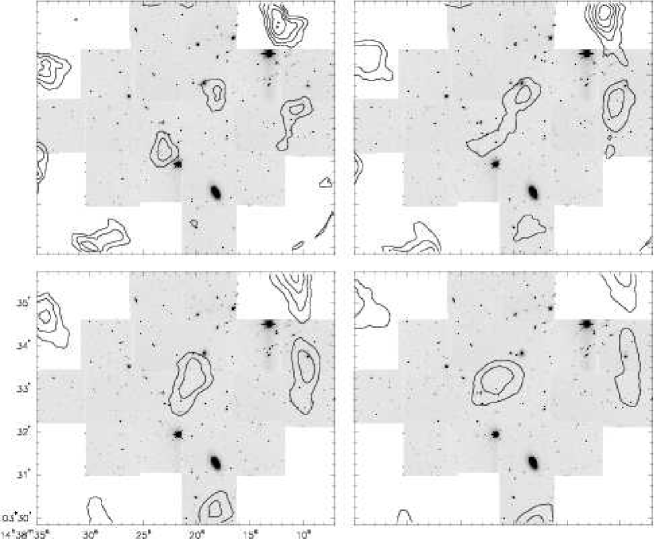
5.5 Projected galaxy density

Figure 16: Projected number density of galaxies in the HST image. The upper left image shows contours of surface densities, smoothed with a Gaussian of width $\sigma=15\arcsec$, for all galaxies in the catalog, starting at 70 arcmin^-2, and increasing in 10 arcmin^-2 intervals. For the other three plots, the galaxy catalog was split as before into magnitude bins. Bright galaxies are shown in the upper right panel, medium bright ones in the lower left, faint ones in the lower right. The contours for these panels start at 25 arcmin^-2, and increase in 5 arcmin^-2 steps.

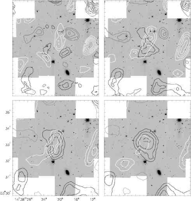
Neither Erben et al. (2000, $I$-band) nor Gray et al. (2001, $H$-band) find a significant overdensity of galaxies which could be associated with the Dark Clump. With the substantially deeper HST data, we can probe the galaxy number density to fainter magnitudes. In Fig. 16, we present surface number densities for the complete galaxy sample, as well as split up according to brightness, as done before for the lensing analysis.

The bin of brightest HST galaxies corresponds roughly to those objects detected also in the ground-based image. It is quite puzzling that rather than an overdensity of galaxies at the dark clump, the galaxies seem to form a ring around that position. However, this is hardly significant.

The most significant feature we find is a $5\sigma$ galaxy overdensity in the bin of medium bright galaxies, located about $1\arcmin$ from the Dark Clump. Given that these objects are fainter than the ones that carry the lensing signal in the ground-based data, this is rather unlikely to be associated with a lensing mass. However, it could explain the alignment signal seen in the faintest HST bin. It would be highly interesting to investigate whether this overdensity is present also in color space; unfortunately, the currently available data sets are not deep enough.

5.6 Summary

We have shown that we also detect tangential alignment around the Dark Clump in the HST data. However, it is considerably less significant than in the ground-based data. It is particularly intriguing that we do not detect alignment in the medium bright HST galaxies.

We refrain from trying to deduce a mass for the dark clump from these measurements, as it is obvious that our results are not unambiguous. As an upper limit, the HST data suggest that the mass estimate of the dark clump has to be corrected at least by a factor of 1/2 compared to the original value.

A comparison on an object-to-object basis may be able to shed some light on the question whether the ground-based lensing signal is only a noise peak or whether there are other, uncorrected problems with the HST mosaic. Such a comparison is carried out in App. B.

6 X-ray analysis

Figure 17: A part of the Chandra image overlaid on the HST image. The point sources were removed from the image, and it was smoothed with a Gaussian of $5\arcsec$. The contour levels start at $3.6\times 10^{-14}$ erg cm^-2 s^-1 and increase in steps of $0.8\times 10^{-14}$ erg cm^-2 s^-1. An increase in X-ray emission due to Abell 1942 (north of the dark clump) is visible. In the vicinity of the dark clump, there is a 1.5$\sigma$ source at $\alpha=14^{\rm h}\,38^{\rm m}\,22.7^{\rm s},\>\delta=3^{\circ}\,32\arcmin\,57\arcsec$ (marked with ${\mathbf{\times}}$) in a circular aperture of radius $45\arcsec$ (indicated).

If the dark clump is a virialized massive dark matter concentration, one would expect that the baryons trapped by the potential well and not in galaxies would have been shock-heated in the gravitational collapse and therefore would emit in X-rays. Erben et al. (2000) present the analysis of the ROSAT HRI image of the A1942 field. They found a hardly significant X-ray detection at a position $60\arcsec$ away from the weak lensing mass peak position reported in that paper.

Since then, the field of A1942 was imaged by the Chandra X-ray observatory in March 2002 (PI: Garmire). It was observed for 58 ks with the ACIS-I detector configuration. We retrieved the observation from the archive and analysed it using standard techniques with the CIAO v3.1 package. and recipes from the “ACIS Recipes: Clean the Data” web page. We use the standard set of event grades (0,2,3,4,6) and restrict our analysis to the 0.5-8.0 keV energy band. We detect sources with CIAO’s WAVDETECT routine using wavelet scales 1, 2, 4, 8 and 16. Only two sources are detected within $100\arcsec$ of the CFHT data lensing $M_{\rm ap}$ centroid. These two sources are found to be point sources with clear optical counterparts in the optical data.

Visual inspection does not reveal any obvious extended source at the position of the dark clump. Nevertheless, in order to check if there really is any extended source, we created a diffuse emission image from our original image excising the data where WAVDETECT detected sources and filling the holes according to CIAO’s threads. We also created a “blank-sky” background image to better estimate the background contribution at the position of the dark clump. We smoothed the point-source-removed image with and without background subtraction with various algorithms and scales but no obvious extended source was detected. The most significant source consistent with the broad position of the dark clump is a 1.5$\sigma$ source (in a circular aperture of radius $45\arcsec$) whose coordinates are $\alpha=14^{\rm h}\,38^{\rm m}\,22.7^{\rm s},\>\delta=3^{\circ}\,32\arcmin\,57\arcsec$. We measure a count-rate of $(5.9\pm 4.0)\times 10^{-4}$ counts/s in the 0.5-8.0 keV energy range in a circular aperture of radius $45\arcsec$ which corresponds to a unabsorbed flux of $(5.3\pm 3.4)\times 10^{-15}$ erg cm^-2 s^-1 assuming an incident spectrum of $T=3$keV and a local hydrogen column density of $N_{H}=2.61\times 10^{20}$ cm^-2. We also measure the count rate in various apertures centered at the positions of the CFHT and HST data lensing centroids. The measurements are of lower significance compared to the previous one. We have fitted a standard beta profile (Cavaliere & Fusco-Femiano 1978) to the azimuthally average radial profile centered at the position of this potential source. We obtain best values for the core radius and beta parameter (slope decline at large radius) of $5\arcsec$ and 0.55, respectively. These values indicate that if there really is an extended source, it is rather compact with a small core radius. Although, one has to keep in mind that these best fit parameters are highly uncertain due to the low number of counts. The total count rate predicted integrating the best-fit model would be $9.4\times 10^{-4}$ counts/s.

Erben et al. (2000) reported a hardly significant ($3.2\sigma$) detection of X-ray emission in the dark clump area in the ROSAT HRI image of this field. We have measured the flux in the Chandra image at the same position, which is very close ($15\arcsec$ away) to the previously reported source. We find an unabsorbed flux of $(6.8\pm 3.6)\times 10^{-15}$ erg cm^-2 s^-1 in a $45\arcsec$ aperture. This value is slightly higher than the previous one only due to the inclusion in the aperture of another faint source situated at the NE and not included in the mesurement at the previous position. Therefore, we do not confirm the flux measurement of the ROSAT HRI source.

Given the faintness and measured uncertainties of our possible detection, there is little point in speculating about the luminosity and gas mass of our possible detection. Even if this source was real and its real flux was the highest allowed by the data, it would not have enough mass to be considered a rich cluster by its X-ray properties. Overall, the Chandra image of this source indicates that if there is a dark matter concentration producing the lensing signal, this concentration does not contain the expected mass of hot gas that would be expected for its lensing signal if it were similar to the clusters of galaxies we have observed so far.

7 Conclusion

Tangential alignment around the dark clump was detected in three datasets, which differ in the filter, camera, and telescope used. It can therefore be ruled out that the alignment is caused by instrument-specific systematics. However, the significance of the detection is lowest in the space-based dataset. If the alignment were due to lensing by a matter concentration, the highest alignment signal would be expected in the HST data, as it extends to more distant galaxies which should be more affected by the distortions due to lensing.

The significant alignment signal in the ground-based data is caused mainly by faint galaxies, for which the individual shape measurement are uncertain due to background noise. We show in App. B that the shape measurements agree very well on average when comparing ground-based and space-based data. Thus, also the amplitude of an alignment signal should be comparable. Considering the high alignment signal in the two ground-based datasets, it seems unlikely that background noise boosted the signal in both cases. Yet, for the $I$-band image, there is some indication of such a “conspiracy”, as the average tangential ellipticity toward the dark clump of the objects compared is significantly larger for the ground-based measurements (see B.4).

There are several issues involved which actually make weak lensing analyses more difficult to apply to HST data (small field-of-view, complicated PSF structure). But various tests (App. A and B.4) have not revealed any bias these problems might cause to the ellipticity measurements. The weaker alignment signal in the HST data is therefore not a result of these systematics.

For the original detection claim, further evidence for a lensing mass was lent by the detection of X-ray emission in a ROSAT HRI image. However, follow-up observations with Chandra measure only a tenth of the flux originally measured in the ROSAT data, making this more likely to be a spurious detection. Thus, if it is a lensing mass, the dark clump would be truly “dark”, not just in the optical.

We cannot give a definite answer to the question of the nature of the Dark Clump candidate found by Erben et al. (2000). It has neither been possible to prove that it is a Dark Matter halo, nor that it is a statistical fluke, caused by noise in either the intrinsic galaxy ellipticities or the measurement process. Our analyses assert that there is indeed tangential alignment around the dark clump. However, it remains unclear whether this is caused by a lensing mass, is just a chance alignment, or a combination of the two.

The lack of signal in the medium magnitude bin of the HST data and the lack of X-ray emission yield the first hypothesis more unlikely (at least compared to Erben et al. (2000)), but not impossible if one is willing to accept the existence of very dark, massive halos.

Appendix A Testing for systematics in the HST data

Despite the lack of seeing due to the Earth’s atmosphere, weak lensing analyses of HST data are not applied straightforwardly. Due to the small field-of-view, there are only few stars available for the anisotropy correction; the pixels of the WFPC2 camera undersample the PSF, and the camera has a notable charge transfer inefficiency. In the following, we investigate the effects and possible bias from these problems.

A.1 Anisotropy correction

Figure 18: The anisotropy correction for Chip 2. On the left, the magnitudes of the 850 objects left in the catalog at this stage are plotted vs. their half-light radii. 33 objects from the stellar sequence were used to determine the stellar anisotropy kernel. The orientation and modulus (multiplied with a factor of 2000 [pixels]) of $\mbox{\boldmath${\rm\chi}$\unboldmath}^{*}$ are shown in the middle top box. The fitted polynomial, evaluated at the position of these stars, is shown in the top right box. In the middle lower box, the ellipticity components of these stars before the anisotropy correction are shown; in the lower right box they are shown after correction.

Figure 19: Same as Fig. 18, but for Chip 3. 31 objects out of 930 were used for the fit.

Figure 20: Same as Fig. 18, but for Chip 4. 30 objects out of 770 were used for the fit.

Hoekstra et al. (1998) showed that a better anisotropy correction (eq. (3)) of WFPC2 images can be achieved if the weight function applied to the stellar images is adapted to the size of the object to be corrected.

However, in practice, the ellipticity measurements become increasingly noisy for larger radii of the weight function. Along with the low number of stars, this causes fits to the anisotropy kernel to be both noisy and ill-described by a simple polynomial.

We tested three possible methods of correcting for the anisotropy as measured from the stars:

1. the anisotropy kernel $\mbox{\boldmath${\rm q}$\unboldmath}^{\star}$ fit to measurements with a weight function of stellar size;

2. the anisotropy kernel $\mbox{\boldmath${\rm q}$\unboldmath}^{\star}(r)$ fit to measurements with a weight function of the objects’ size $r$;

3. a factor $a$ is applied to $\mbox{\boldmath${\rm q}$\unboldmath}^{\star}$ to minimize the difference to the stellar ellipticities measured at the objects’s size.

The third method acknowledges that the anisotropy kernel is a function of object size, but avoids the uncertainties from fitting a polynomial to the noisy measurements with a larger weight function. However, it can only compensate for variations in the PSF that are uniform across the chip and of the same magnitude in both ellipticity components.

The anisotropy patterns produced by these methods are indeed notably different. But the resulting shear estimates $\varepsilon$ differ only on a percent level. Accordingly, the $M_{\rm ap}$ measurements change only minutely with a different anisotropy correction. We used the third method as a compromise solution.

The fits to $\mbox{\boldmath${\rm q}$\unboldmath}^{\star}$ are illustrated in Figs. 18 - 20. For each chip, about 30 stars are available for the anisotropy correction. This is a very small number, and as can be seen from the Figures, they are not evenly distributed over the chip. It is therefore difficult to judge the quality of the anisotropy correction.

Alternatives? It is common to use globular cluster fields for the anisotropy correction rather than the few stars contained in the field itself. With the large number of stars, the anisotropy can be very well determined. However, such fields have to be chosen carefully: they should have been taken temporally close to our field, have a similar dither pattern, and should have been taken in the same filter. As it turned out, no images of star clusters, M31, M33, the Magellanic Clouds, or galactic fields were taken with the F702W filter in 2000 - 2002.

Instead, we retrieved images of a field within the globular cluster 47 Tuc (NGC 104) taken in the F606W filter on Oct. 19th, 2002. We found the anisotropy patterns of these images to be similar to the ones in our images, but with some notable differences. Using these patterns for the anisotropy correction did not reduce the ellipticity dispersion of the stars (see Fig. 21). At least for the centers of the images, the previous method is therefore superior. However, due to a lack of stars, the anisotropy correction is largely extrapolated toward the edges of each chip. These are also the areas with the largest anisotropy (as apparent from the figures), so that we are uncertain of the quality of the anisotropy correction applied to them.

Figure 21: Anisotropy correction of Chip 3. In the top left field, we plot the ellipticities of the 33 stars from the stellar sequence (as in Fig. 19). Their ellipticity components are shown in the bottom left panel. In the top middle panel, we evaluate the anisotropy kernel as found from these 33 stars on a grid. The residual ellipticities of the stars after correction are shown in the bottom middle panel. In the top right panel, the correction polynomial found from 372 stars in a star cluster field is shown. Applying this polynomial to our data yields the residual ellipticities shown in the lower right panel.

A.2 Charge Transfer Efficiency

Figure 22: The average ellipticity components as a function of distance from the read-out amplifier. As before, the galaxies are split into magnitude bins, where circles denotes the faintest, triangles the medium bright ones, and squares the brightest. $\langle\tilde{\varepsilon}_{1}\rangle$ is shown as solid symbols with solid error bars, $\langle\tilde{\varepsilon}_{2}\rangle$ as open symbols with dashed error bars. The error bars denote the standard deviation divided by the square root of the number of galaxies to give the significance of the mean value.

WFPC2 has a considerable Charge Transfer Efficiency (CTE) problem. Stars bright enough to show diffraction spikes also show typical “CTE tails” in the direction opposite to the read-out direction. In fainter objects, these tails are not distinguishable by eye. Unfortunately, this effect is difficult to compensate for and has been studied only little for extended objects (Riess 2000).

The imperfect CTE of the WFPC2 could potentially bias the measured ellipticities, since it results in charge being depleted in some pixels and added into others. Unlike for the photometry of point sources, there is not yet a correction procedure to account for this effect for shape measurements. According to Riess (2000), for extended objects, the A deficient CTE causes charge loss in the pixels closer to the read-out amplifier but adds this charge to the pixels farther from the amplifier. To first order, this just causes a slight displacement of the galaxy’s centroid. But since depletion and addition cannot be expected to be symmetric, it may also distort the galaxy’s shape. If so, it would bias the $\varepsilon_{1}$ components, as this is measured along rows and columns.

From studies on how CTE affects photometry it is known that it increases with distance from the read-out amplifier. This is also visible in our images: stars with large $y$-coordinates have more pronounced CTE trails. Also, the charge loss due to CTE depends on the background level of the image. A high background effectively suppresses CTE losses. The images of our dataset have a background corresponding to about 35 electrons per pixel, which reduces CTE loss significantly, at least for photometry. Lastly, the relative CTE losses are largest for faint objects.

To investigate any possible bias due to CTE, we divide the galaxy catalog into four bins according to the original $y$ position, which gives its distance from the amplifier. Unlike for the lensing analysis, we are not interested in the ellipticity with respect to the rectascension axis, but to the original $x$-axis of the image. We denote these with $\tilde{\varepsilon}_{i}$. For each bin, we calculate the weighted mean of $\tilde{\varepsilon}_{1}$ and $\tilde{\varepsilon}_{2}$. The results are shown in Fig. 22.

If the CTE would affect galaxies similar to stars, i.e. it causes them to trail and thus elongates them in the $\tilde{\varepsilon}_{1}$ direction, we would expect that $\langle\tilde{\varepsilon}_{1}\rangle$ is consistent with zero for the first bin and then decreases with increasing distance from the amplifier. This is clearly not the case for any of the brightness bins. The scatter in $\langle\tilde{\varepsilon}_{1}\rangle$ about zero is comparable to that in $\langle\tilde{\varepsilon}_{2}\rangle$, which should not be affected by CTE. The deviations from zero in some bins may well be due to the fact that there is some degree of tangential alignment in the field, so that $\langle\tilde{\varepsilon}_{1}\rangle$ and $\langle\tilde{\varepsilon}_{2}\rangle$ are not necessarily zero. Yet, Fig. 22 excludes a notable bias due to CTE.

Appendix B Comparison of ground-based and space-based measurements

With the two datasets - the $I$-band image and the HST image - we have the opportunity to directly compare shape measurements from the ground to those from space. Ground-based shape determinations rely on an accurate compensation of the smearing due to the Earth’s atmosphere, while the HST observations are hampered by the small image size, and the undersampling of the PSF. In the previous section, we confirmed with the HST data the presence of tangential alignment around the dark clump candidate, which implies that ellipticity measurements are to some degree comparable. However, we failed to confirm with the HST data the amplitude of the alignment signal.

A direct comparison of the objects common to both catalogs tests the reliability of ground-based shape measurements and may also help to identify any systematics in either dataset. The ultimate goal of this comparison is to find the cause of the discrepancy in the significance of the alignment signal between the two datasets.

B.1 Catalog correlation

As the HST data was astrometrically calibrated by using a reference catalog extracted from the $I$-band image, objects present in both images can be identified by their sky coordinates.

To correlate the catalogs, we searched for objects within $1\arcsec$ of objects detected in the respective other catalog. This radius was found to be the optimal balance between a high number of matched objects and a low rate of double detections.

The catalogs used are the same as those for the lensing analysis, except that objects with $P^{g}_{s}<0.3$ in the ground-based catalog are also considered.

Within the field covered by the HST mosaic, there are 507 objects in the $I$-band catalog. We find one HST counterpart for 350 of these objects, and two or three counterparts for 17 objects, as the HST is able to resolve very close objects which were identified as single objects in the ground-based data. For 140 objects, no counterpart was found. For most of these, this results from the large areas that were masked in the HST images.

Figure 23: The magnitudes and half-light radii of the $I$-band objects positioned in the field observed by the HST. Open circles denote objects for which one HST counterpart was found, solid ones no counterpart, and crosses more than one counterpart. For some of the bright, large objects no counterpart was found due to the large masked areas in the HST mosaic.

Fig. 23 illustrates the matched objects in an $r_{g}-m$ diagram of the ground-based data. There is no apparent trend as to for which objects we are more likely to find a counterpart in the space-based data. In particular, it is not less likely to do so for faint objects. This shows that the catalog was only very little contaminated by noise detections. Since close objects are often unresolved in the ground-based image, objects with two HST counterparts have on average a larger radius than those with one counterpart.

B.2 Statistical properties

B.2.1 Ellipticity measurements

The basis of weak lensing analyses are the shape measurements of faint galaxy images. But the fainter an object is, the more difficult the shape determination is. Our dataset provides an ideal opportunity to test the reliability of shape measurements of ground-based data compared to space-based measurements.

Figure 24: Comparison of the ellipticity measurements from the HST images to the $I$-band image. Objects for which $\Delta\varepsilon\leq 0.2$ [see eq. (20)] are shown as solid circles, objects with $\Delta\varepsilon>0.2$ are shown as open circles. The line gives the best linear fit. The error bars of individual points are omitted to avoid crowding.

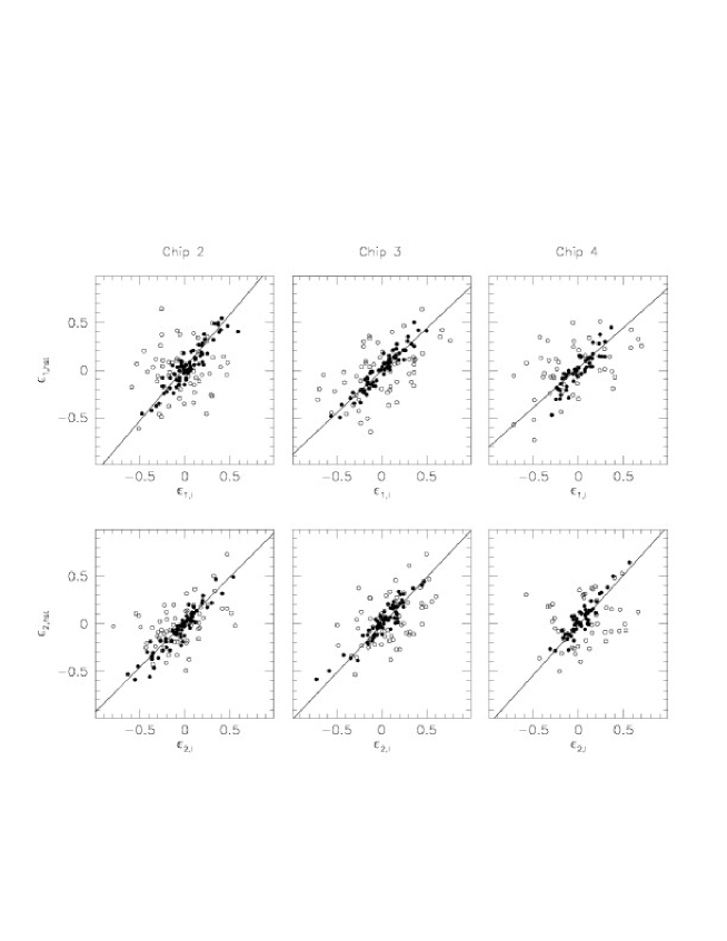
In Fig. 24, we compare the ellipticity measurements in the space-based data to those of the ground-based data. To these points, we fit a linear function (algorithm fitexy from Press et al. 1992, to account for errors in both coordinates), where we employ the same weighting scheme as applied to the lensing analysis. We find:

$$\begin{array}[]{r@{\;=\;}l@{\qquad\qquad}r@{\;=\;}l}\varepsilon_{1,\rm hst}&m_{1}\cdot\varepsilon_{1,\rm I}+b_{1}&\varepsilon_{2,\rm hst}&m_{2}\cdot\varepsilon_{2,\rm I}+b_{2}\\[4.30554pt] m_{1}&0.94\pm 0.14&m_{2}&0.97\pm 0.15\\ b_{1}&0.017\pm 0.027&b_{2}&-0.001\pm 0.027\end{array}$$

Although the scatter is rather large and a comparison on an object-to-object basis not feasible, the general agreement for the is very good, particular for the $\varepsilon_{2}$ component. For the $\varepsilon_{1}$ component, both slope and offset $b_{1}$ differ from unity by about $0.5\sigma$. If the HST ellipticity measurements are influenced by the CTE problem or by the resampling of the drizzle algorithm, we would indeed expect some bias in the $\varepsilon_{1}$ component, which is measured along the rows and columns of the CCD chip.

The scatter seen in the correlation of both components is of a similar order of magnitude, so that the deviations in the ellipticity measurements cannot be attributed to a single component. For simplicity, we therefore reduce the difference of the ellipticity measurements to a one-dimensional quantity:

$$\Delta\varepsilon=\sqrt{(\varepsilon_{1,\rm hst}-\varepsilon_{1,\rm I})^{2}+(\varepsilon_{2,\rm hst}-\varepsilon_{2,\rm I})^{2}}$$ (20)

Ellipticity measurements are considered to be equivalent if $\Delta\varepsilon\leq 0.2$ and inconsistent if $\Delta\varepsilon>0.2$. In the first sample, there are 185 galaxies, whereas in the second there are 165.

B.2.2 Magnitudes

Figure 25: Magnitude measured in the HST data vs. magnitude measured in the $I$-band image for the matched objects. The symbol coding is identical to that of Fig. 24. The dashed lines indicate the cuts used to divide the respective catalogs into three samples.

For the lensing analyses, the galaxy catalogs were split into three parts according to brightness to investigate their contribution to the lensing signal. The division was chosen such that each sample contained an equal number of galaxies. With the merged catalog, we can now examine how these samples compare in the two datasets.

Fig. 25 illustrates the magnitudes measured of the matched objects. Most of the objects found in the $I$-band image are considered “bright” objects in the HST data. The fact that we also detected tangential alignment in the bright HST bin confirms the lensing signal seen in the ground-based image.

As would be expected, the shape measurements agree best for the brighter objects, while they are inconsistent for most of the faint objects.

B.2.3 $P^{\rm g}_{s}$ correction

One quality attribute we used previously to classify objects was the factor $P^{\rm g}_{s}$ by which the smearing due to the PSF was corrected. In Fig. 26 we plot an $r_{g}-P^{\rm g}_{s}$ diagram of the objects found in the $I$-band image within the field covered by the HST mosaic. There is only a slight indication that ellipticity measurements with $P^{\rm g}_{s}<0.4$ are less reliable than others.

Figure 26: The ellipticity correction factor $P^{\rm g}_{s}$ and half-light radii of the $I$-band objects within the HST field. Crosses denote objects for which no counterpart was found; the other colors are the same as in Fig. 24.

B.2.4 Signal-to-noise ratio and weighting

Two other criteria for the reliability of a shape measurement are the signal-to-noise ratio of a detection and the weight it was assigned. The latter one was taken to be inversely proportional to the variance $\sigma^{2}$ of the ellipticities of a galaxy ensemble with similar noise properties [see Sect. 2.3.9]. Fig. 27 shows the signal-to-noise ratios and weights of the $I$-band objects in the HST field.

Figure 27: The signal-to-noise ratios snr and weights of the $I$-band objects in the HST field. The color-coding is identical to that of Fig. 26.

As expected, the ellipticity measurements deviate for those objects with a low signal-to-noise ratio. These are in general down-weighted, although the weight itself is not a clear indicator of the reliability. The weighting scheme could therefore be improved.

The lensing signal in the ground-based data was carried by faint galaxies with a signal-to-noise ratio of less than about 4. These are precisely those galaxies for which the space-based measurements give different ellipticities. It is therefore not surprising that the amplitude of the $M_{\rm ap}$ signal is different in the two datasets.

B.2.5 Dependence on chip position

Figure 28: Ellipticity differences $\Delta\varepsilon_{1}$ and $\Delta\varepsilon_{2}$ as a function of position in the HST mosaic. Plotted on the $x$-axis is the distance from the chip center (measured in pixel units after the drizzle process); objects detected on Chip2 are shown as circles, Chip3 as triangles, and Chip4 as crosses. The distinction we make between equivalent and inconsistent shape measurements is illustrated by the black, long-dashed lines (if for the respective other component $\Delta\varepsilon_{i}=0$). The dotted, short-dashed, and dot-dashed lines give linear fits to the respective data.

As mentioned before, we cannot judge the quality of the anisotropy correction of the HST images due to the small number of stars in the images. With the correlated catalogs, we have another test of the correction: if it is faulty, then we expect to see a systematic variation of the ellipticity differences $\Delta\varepsilon_{1}=(\varepsilon_{1,\rm hst}-\varepsilon_{1,\rm I})$ and $\Delta\varepsilon_{2}=(\varepsilon_{2,\rm hst}-\varepsilon_{2,\rm I})$ between the three chips and/or with position on the chip. We reduce the latter one to a one-dimensional quantity by considering the distance $r$ from the respective chip center; this is motivated by the observation that the anisotropy seen in the HST chips is largest at the edge (see Fig. 21).

In Fig. 28 we plot $\Delta\varepsilon_{1}$ and $\Delta\varepsilon_{2}$ as a function of $r$, where we distinguish between the three chips. Clearly, an object’s position in the HST mosaic is not the main cause of discordance in the ellipticity measurement. However, there are trends visible such as a slight overestimation of $\varepsilon_{1}$ for small $r$ in Chip 4 and an underestimation of $\varepsilon_{1}$ for small $r$ in Chip 3. To quantify these, we fit a linear function $\Delta\varepsilon_{i}=m_{i}\cdot r/1000+b_{i}$, for each chip. We weight the $\Delta\varepsilon_{i}$ values by the same weighting scheme as before, but do not assign error bars to the distance. The results are:

$$\begin{array}[]{l@{\qquad}c@{\qquad}c@{\qquad}c}&\mbox{Chip 2}&\mbox{Chip 3}&\mbox{Chip 4}\\[5.16663pt] m_{1}&-0.21\pm 0.17&0.23\pm 0.16&0.14\pm 0.19\\ b_{1}&0.14\pm 0.10&-0.13\pm 0.10&-0.05\pm 0.11\\[4.30554pt] m_{2}&0.05\pm 0.17&0.02\pm 0.16&0.03\pm 0.19\\ b_{2}&-0.01\pm 0.10&-0.02\pm 0.10&-0.03\pm 0.11\end{array}$$

For the $\varepsilon_{2}$ component, the ellipticity difference is remarkably constant at zero for all chips. However, for the $\varepsilon_{1}$ component, there is a significant deviation from such a behavior in Chips 2 and 4. The anisotropy pattern of the HST chips is approximately circular in appearance (see Fig. 21), so that an insufficient anisotropy correction should affect both components equally. The deviation in $\varepsilon_{1}$ may therefore be a hint that the CTE and / or the drizzle process affect the ellipticities systematically. On the other hand, the linear fits are certainly noisy due to the small number of objects, particularly at low $r$.

Considering that $\Delta\varepsilon_{2}$ is on average constant at zero, but also that $\Delta\varepsilon_{1}$ is consistent with zero for a large number of objects ($400<r<800$), strengthens our assumption that the anisotropy correction worked properly.

B.3 Lensing analysis

Figure 29: $M_{\rm ap}$ analysis of the 350 objects common to both the ground- and the space-based catalog. The upper two panels show $M_{\rm ap}$ contours, starting at 0.02 and increasing in 0.02 increments, where a filter scale of $80\arcsec$ was used for the left panel, and a filter scale of $120\arcsec$ for the right one. The lower two panels give signal-to-noise contours, starting at 1.5$\sigma$ and increasing in 0.5$\sigma$ increments. The white contours correspond to the analysis using ground-based ellipticities, and black ones to the one using space-based ellipticities.

Since the ellipticity measurements agree on average, one can assume that the lensing analysis of our set of matched objects should yield similar results. However, the individual analyses indicate otherwise: the faint galaxies in the ground-based data, which caused most of the lensing signal, correspond to the bright (and medium bright) galaxies in the HST data, which gave only a weak signal.

In order to directly evaluate the correlation (or discrepancy) between the ellipticity measurements and the lensing analysis, we perform several $M_{\rm ap}$ analyses of the matched galaxies (see Table 4 for a quantitative summary).

As a reference, we perform a $M_{\rm ap}$ analysis of the 350 matched objects using once the ground-based ellipticity measurements and once the space-based measurements (Fig. 29). It is quite remarkable how well the $M_{\rm ap}$ contours agree for these; however, for the dark clump peak, the space-based values reach only half the height of the ground-based.

Figure 30: $M_{\rm ap}$ analysis of objects with $\Delta\varepsilon\leq 0.2$ (left side) and $\Delta\varepsilon>0.2$ (right side). The upper panels show the $M_{\rm ap}$ values measured in the $120\arcsec$ filter scale, the lower ones the corresponding signal-to-noise ratios. The color coding and the contours are identical to Fig. 29.

Restricting the galaxy sample to those for which $\Delta\varepsilon\leq 0.2$ further highlights the agreement, as is expected (left hand side of Fig. 30). These are mainly the galaxies considered “bright” also in the ground-based image (see Fig. 25), which contribute to the lensing signal found there. Even for these, the $M_{\rm ap}$ values of the dark clump peak are a factor of 1.4 higher for the ground-based ellipticity measurements.

For the $120\arcsec$ scale, the discrepancy in the $M_{\rm ap}$ measurements at the dark clump position is even larger for those objects with $\Delta\varepsilon>0.2$ (right hand side of Fig. 30). In the ground-based data, there is a $>3.7\sigma$ peak slightly to the right of the dark clump position, while the $M_{\rm ap}$ values in the space-based data are comparable to the $\Delta\varepsilon\leq 0.2$ sample, with a significance of $\sim 2\sigma$. At the dark clump position, the amplitudes in the ground-based values are on average a factor 3 larger than the space-based ones for all filter scales. Interestingly, for the smallest two filter scales, the highest significance found in the vicinity of the dark clump is equivalent in the two datasets. However, this is based only on a very small number of galaxies.

Table 4: Overview of the $M_{\rm ap}$ analyses discussed in this appendix. Shown are the results at the position of the dark clump as measured in the ground-based data, since we want to determine the cause of the high $M_{\rm ap}$ amplitude in the ground-based data at this position. We list the ellipticity dispersion, the $M_{\rm ap}$ value itself, and the signal-to-noise ratio. For those analyses of the 350 matched objects, we give both the results of using the ground-based and of using the space-based data. For the second block from the bottom of the table, the ground-based analysis uses the space-based weights and vice versa. For the last block, the $\varepsilon_{1}$ component of the HST measurements is modified by applying the inverse of the linear fit between space-based and ground-based ellipticities. Evaluating $M_{\rm ap}$ only at the ground-based dark clump position biases the result in favor of larger ground-based values. For a better comparison of the general values, we quote the highest significance found in the vicinity of this position in parentheses.

	$\theta_{\rm out}$	N	$\sigma_{\varepsilon}$(I)	$\sigma_{\varepsilon}$(HST)	$M_{\rm ap}$(I)	$\!M_{\rm ap}$(HST)	SNR(I)	SNR(HST)
all objects of	80$\arcsec$	119	0.34	-	0.056	-	2.6 (3.8)	-
ground-based	100$\arcsec$	178	0.34	-	0.070	-	3.5 (4.4)	-
catalog in	120$\arcsec$	267	0.35	-	0.076	-	4.8 (4.8)	-
HST field	140$\arcsec$	364	0.34	-	0.061	-	4.5 (4.6)	-
objects with	80$\arcsec$	76	0.33	0.32	0.064	0.017	2.4 (4.0)	0.6 (2.5)
1 counterpart	100$\arcsec$	123	0.34	0.32	0.088	0.040	3.8 (4.6)	1.8 (2.7)
	120$\arcsec$	181	0.34	0.32	0.087	0.043	4.6 (4.6)	2.3 (2.8)
	140$\arcsec$	148	0.34	0.32	0.065	0.025	4.0 (4.0)	1.6 (2.2)
$\Delta\varepsilon\leq 0.2$	80$\arcsec$	43	0.27	0.29	0.041	0.014	1.4 (3.0)	0.4 (2.6)
	100$\arcsec$	68	0.27	0.28	0.065	0.041	2.4 (3.1)	1.4 (2.5)
	120$\arcsec$	95	0.28	0.28	0.074	0.050	3.2 (3.3)	2.2 (2.4)
	140$\arcsec$	135	0.28	0.29	0.046	0.035	2.5 (2.9)	1.9 (2.4)
$\Delta\varepsilon>0.2$	80$\arcsec$	33	0.42	0.36	0.105	0.022	2.0 (2.8)	0.5 (3.2)
	100$\arcsec$	55	0.42	0.37	0.127	0.038	3.0 (3.5)	1.0 (2.2)
	120$\arcsec$	86	0.42	0.36	0.106	0.034	3.2 (3.8)	1.1 (2.1)
	140$\arcsec$	113	0.42	0.36	0.095	0.012	3.1 (3.4)	0.5 (2.2)
weights	80$\arcsec$	76	0.35	0.32	0.067	0.019	2.3 (3.6)	0.7 (2.6)
swapped	100$\arcsec$	123	0.35	0.32	0.093	0.040	3.7 (4.4)	1.7 (3.0)
	120$\arcsec$	182	0.36	0.31	0.095	0.048	4.6 (4.7)	2.6 (3.2)
	140$\arcsec$	249	0.35	0.32	0.073	0.030	4.2 (4.3)	1.9 (2.6)
HST $\varepsilon_{1}$	80$\arcsec$	76	-	0.32	-	0.017	-	0.6 (2.5)
component	100$\arcsec$	123	-	0.32	-	0.040	-	1.8 (2.7)
adjusted	120$\arcsec$	182	-	0.32	-	0.043	-	2.3 (2.8)
	140$\arcsec$	249	-	0.32	-	0.025	-	1.6 (2.2)

As there is a $M_{\rm ap}$ peak in all these samples, we can be sure that there is some tangential alignment around the dark clump candidate. But it is still unclear why it is measured to be so much larger in the ground-based image.

B.3.1 Interchanging the weights

For the lensing analysis, the entries in the ground-based and space-based catalogs differ mainly in the shape measurements and in the weights assigned to each object. We have shown that the ellipticity measurements agree on average, but we have not yet considered the different weights assigned.

Figure 31: A comparison of the weights assigned to the matched objects in the HST catalog and the ground-based catalog. Again, solid points denote objects with $\Delta\varepsilon\leq 0.2$, open circles $\Delta\varepsilon>0.2$.

In Fig. 31, we directly compare the weights assigned to the matched objects. Certainly, objects which were down-weighted in the ground-based data have higher weights in the HST catalog. But else, the scatter is fairly large.

To test the influence of the weights on the lensing analyses, we perform an analysis where we interchange the weights, i.e. we assign to each object in the ground-based image the weight of its counterpart in the HST image and vice versa. The results are listed in Table 4. It is interesting to note that at most filter scales, this causes the ground-based value to decrease and the space-based value to increase. But the $M_{\rm ap}$ values are within the error bars of the ones with the original weights and are therefore only slightly dependent on the weights.

B.3.2 Recalibrating the HST $\mbox{\boldmath${\rm\varepsilon}$\unboldmath}_{1}$ component

We noted earlier that the linear fit applied to the $\varepsilon_{1}$ components of the matched objects yields a $y$-intercept with almost $1\sigma$ significance (Sect. B.2.1). This might point to a problem of the HST data related to its CTE or the drizzle procedure.

Earlier, the ellipticity measurements from all three chips were considered. The ellipticities compared were those defined with respect to the rectascension axis. However, any problem regarding the CTE would bias the ellipticity measurements with respect to the read-out direction, which is different for all three chips. Also, the effect of the anisotropy correction is likely to be different for each chip.

Figure 32: Comparison of the ellipticity measurements in the HST image and the $I$-band image, separated by HST chip. The upper row shows the $\varepsilon_{1}$ measurements, the lower the $\varepsilon_{2}$ measurements. Filled circles denote objects with $\Delta\varepsilon\leq 0.2$, open ones $\Delta\varepsilon>0.2$. A weighted linear fit is indicated by the solid line.

Therefore, we repeat the ellipticity comparison for the matched objects separated according to which HST chips they were measured in. The linear fits yield (with the same definition of the fit-parameters as in Sect. B.2.1):

$$\begin{array}[]{l@{\qquad}c@{\qquad}c@{\quad}c}&\mbox{Chip 2}&\mbox{Chip 3}&\mbox{Chip 4}\\[5.16663pt] m_{1}&1.09\pm 0.31&0.89\pm 0.21&0.83\pm 0.22\\ b_{1}&0.035\pm 0.047&-0.006\pm 0.043&0.032\pm 0.047\\[4.30554pt] m_{2}&0.97\pm 0.23&1.01\pm 0.25&1.07\pm 0.32\\ b_{2}&0.015\pm 0.045&-0.010\pm 0.047&-0.015\pm 0.054\end{array}$$

For the $\varepsilon_{2}$ component, the agreement is still very good for all three chips. For the $\varepsilon_{1}$ component, the deviations from a slope of unity are larger. Particularly, Chip 2 and 4 exhibit a notable non-zero $y$-intercept. If these deviations are indeed a result of systematics in the HST data, applying the inverse relation to the HST measurements should then on average retrieve the ground-based ellipticities.

We modify the HST measurements by the relation

$$\varepsilon_{1}\quad\longrightarrow\quad\frac{\varepsilon_{1}-b_{i}}{m_{i}}$$

for each chip $i$. We do not alter the $\varepsilon_{2}$ components, as we deem their agreement with the ground-based data satisfactory.

The results of a lensing analysis of the matched objects with these modified ellipticities are listed in Table 4. Indeed, this transformation yields $M_{\rm ap}$ values 25% larger than the original ones for the smallest two filter scales. For the $100\arcsec$ filter scale, the effect is smaller, and for the $120\arcsec$ filter scale it is negligible.

If the height of the $M_{\rm ap}$ peak were uncorrelated with the systematic deviation in the ellipticity measurement, the modification would only add noise to the $M_{\rm ap}$ statistic, as most ellipticities are amplified due to $m_{i}<1$. The $M_{\rm ap}$ value of the peak therefore would not be significantly altered, as is the case at least for the largest filter scale. For the other filter scales, there is a slight increase in both $M_{\rm ap}$ and SNR value. But the change is at most $0.3\sigma$, so the variations are still within the standard deviation of the original measurement.

The results of a lensing analysis of the complete HST catalog with this modification of the ellipticity are very similar to the original one. But as the linear fit which was the basis of this modification applies only to bright objects in the HST catalog, it is very speculative to extrapolate this to fainter objects.

As this modification alone is not able to reproduce the large lensing signal seen in the ground-based data, particularly at the $120\arcsec$ filter scale, the offset of the space-based ellipticities is not the cause of the discrepancy in the $M_{\rm ap}$ measurements.

B.3.3 Rebinning the galaxies in the HST catalog

For the lensing analysis of the HST data, we had divided the galaxy sample into three magnitude bins of equal numbers of object. About half of the objects in the brightest bin were also detected in the $I$-band image and are used in the comparisons presented in this chapter. For these, we have confirmed the presence of tangential alignment, even though the $M_{\rm ap}$ amplitude differs in the two datasets. But we fail to detect alignment in the medium bright HST bin.

The completion limit of the ground-based image falls within the brightest HST bin (cf. Fig. 25), and so a number of objects in the latter, though of similar brightness, were not detected in the ground-based image. To test how much the additional objects in the HST image contribute to the lensing signal, we rearrange the HST brightness bin: instead of the magnitude cut between the brightest and medium bin, we split the galaxies according to whether or not they are a counterpart of an object detected in the $I$-band image. From the latter sample the faintest bin is split with the same magnitude cut as before. This effectively moves several objects from the bright into the medium bin and only a few the other way. The faint bin remains almost unaltered.

Figure 33: $M_{\rm ap}$ analysis of the HST data, with the galaxies split into three samples according to whether they are a counterpart of an object detected in the $I$-band image (white contours). Those objects not detected in the $I$-band image are split by a magnitude cut at $m=26.5$, where gray contours corresponds to galaxies brighter than this limit, black contours to those fainter. The contours start at $1.5\sigma$ and increase in $0.5\sigma$ increments. The filter scales are 80$\arcsec$, 100$\arcsec$, 120$\arcsec$, and 140$\arcsec$ (from upper left to lower right).

In Fig. 33, we present the signal-to-noise contours of a $M_{\rm ap}$ analysis of these three bins. The medium bin, i.e. galaxies brighter than $m=26.5$ that were not detected in the ground-based image contains the most galaxies (835 compared to 350 in the bright bin and 594 in the faint bin), so that the noise is smallest. Yet, the $M_{\rm ap}$ values in the vicinity of the dark clump are compatible with zero within $1\sigma$.

Apparently, there is no tangential alignment present in the objects that were moved from the bright bin to the medium bin. This is compliant with the observation that for those objects also detected in the $I$-band image, the signal-to-noise ratio of the $M_{\rm ap}$ peak is larger than for the bright magnitude bin (cf. Fig. 11).

Intriguingly, this implies that of the faint galaxies at the completion limit of the $I$-band image, those with a tangential alignment to the dark clump were preferentially detected. However, the fact that there is no tangential alignment for about half of the objects in the HST image, which are neither at the bright nor the faint end of the magnitude distribution, clearly disfavors the hypothesis that the tangential alignment in the brighter galaxies is caused by a lensing mass.

B.4 Comparison of the tangential ellipticities

So far, we have not found any systematic that could be the single cause for the discrepancy in the lensing analyses. However, it is clear that for the faint galaxies which mainly caused the lensing signal in the ground-based image, the ellipticities agree with the HST measurements only on average, but not on an object-to-object basis. This is not surprising as the noise in the ground-based image is likely to influence the shape measurements. Yet, it is unlikely that noise can cause (or amplify) tangential alignment around a certain point.

Figure 34: Comparison of the tangential ellipticities measured toward the dark clump (as measured in the ground-based data) of space-based and ground-based objects. Objects with $\Delta\varepsilon\leq 0.2$ are shown as solid, objects with $\Delta\varepsilon>0.2$ as open circles. The dashed line indicates a linear fit to the first sample, the dotted line one to the latter sample. The solid line represents the fit to the combined set.

In Fig. 34 we compare the tangential ellipticity $\varepsilon_{\rm t}$ of the matched objects with respect to the dark clump centroid found in the ground-based data. Only objects within $120\arcsec$ of that position are shown. Evidently, most objects in the ground-based data have a positive $\varepsilon_{\rm t}$. The scatter is comparable to the comparison of the individual ellipticity components (Sect. B.2.1). Likewise, we fit a linear function, where we distinguish between the complete sample of matched galaxies and how well the ellipticity measurements agree (as before, the fit is expressed such that the ground-based data are the independent variable):

$$\begin{array}[]{l@{\qquad}c@{\qquad}c@{\quad}c}&\mbox{all}&\Delta\varepsilon\leq 0.2&\Delta\varepsilon>0.2\\ m&0.98\pm 0.21&1.03\pm 0.28&0.93\pm 0.32\\ b&-0.047\pm 0.043&-0.018\pm 0.055&-0.086\pm 0.071\end{array}$$

For each of these fits, the $y$-intercept is negative, which indicates larger ground-based values. While it lies well within the error bars of the fit for those galaxies with $\Delta\varepsilon\leq 0.2$, it is significantly non-zero for those with $\Delta\varepsilon>0.2$. For those, also the slope indicates a preferentially larger $\varepsilon_{\rm t}$ value in the ground-based data.

On the basis of the correlation of the individual measurements of the tangential ellipticity, the agreement between the two datasets is comparable to that of the ellipticity components, as would be expected. Yet, the mean tangential ellipticity is different: for the ground-based data, it is $\langle\varepsilon_{\rm t,I}\rangle=0.086\pm 0.017$, for the space-based data, $\langle\varepsilon_{\rm t,hst}\rangle=0.034\pm 0.017$. These are very similar to the results of the $M_{\rm ap}$ analysis at the same position at the $120\arcsec$ filter scale, $M_{\rm ap}^{I}(120\arcsec)=0.087\pm 0.019$ and $M_{\rm ap}^{\rm hst}(120\arcsec)=0.043\pm 0.019$ (compare Table 4). This again demonstrates that the coherent alignment is present over a range of distance from the dark clump, as the $M_{\rm ap}$ statistics is a weighted average tangential ellipticity, where the weight is dependent on the distance.

Within the standard deviations of the cited values, the two analyses are compatible with each other. However, these errors are not independent, as they are based on the ellipticity dispersion of the same galaxies. To estimate the significance with which the ground-based mean is larger than the space-based mean, we perform a bootstrap analysis, i.e. from the 195 galaxies in the sample, we draw at random 195 objects, with replacement. From these we calculate $\langle\varepsilon_{\rm t,I}\rangle$ and $\langle\varepsilon_{\rm t,hst}\rangle$ and repeat the procedure 1,000,000 times. The result is shown in Fig. 35. We find that the space-based mean exceeds the ground-based mean in only 176 cases, i.e. the latter one is larger with $3.8\sigma$ confidence.

Figure 35: Results of a bootstrap analysis of the mean tangential ellipticity of the matched objects within $120\arcsec$ of and with respect to the dark clump position in the ground-based data. For objects below the long-dashed line, $\langle\varepsilon_{\rm t,I}\rangle>\langle\varepsilon_{\rm t,hst}\rangle$, above it, $\langle\varepsilon_{\rm t,I}\rangle<\langle\varepsilon_{\rm t,hst}\rangle$. The solid black (red) line and dashed black (red) line indicate $\langle\varepsilon_{\rm t,I}\rangle$ ($\langle\varepsilon_{\rm t,hst}\rangle$) without bootstrapping.

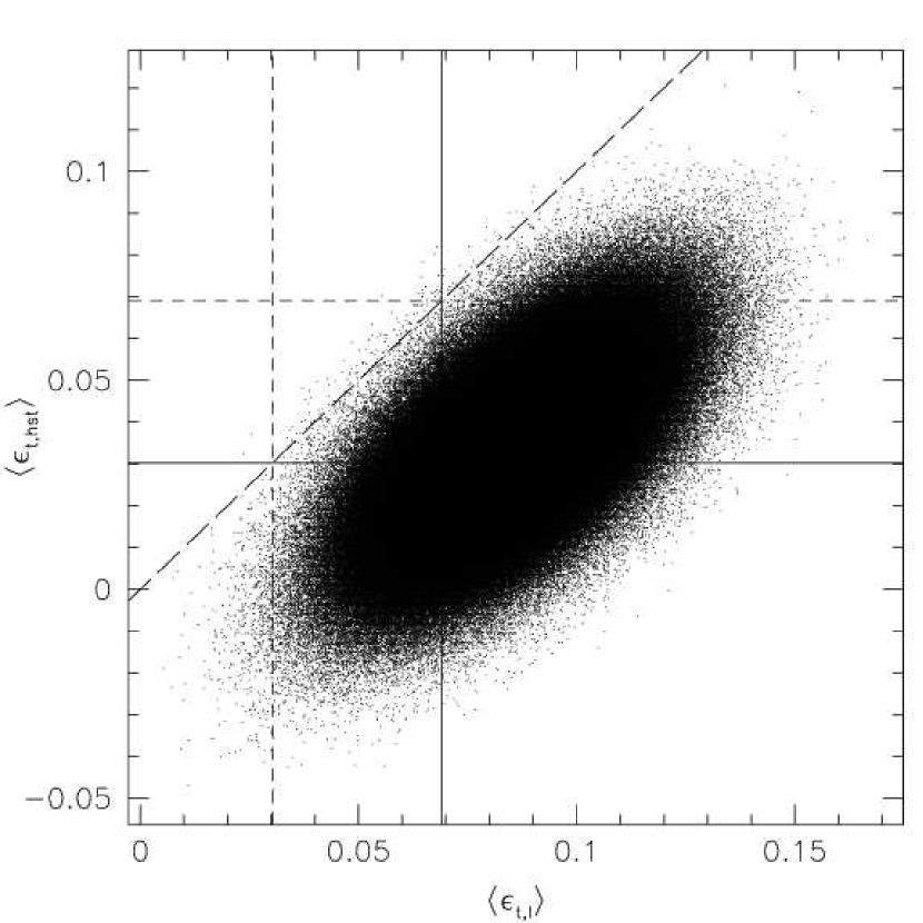
This analysis is biased in the way that the reference position is the dark clump position as measured in the ground-based data. Therefore, we repeat the analysis for the centroid found in the space-based data. Even for this case, the ground-based mean value exceeds the space-based mean with $3.1\sigma$ confidence.

It is quite puzzling that despite the general agreement of the ellipticity measurements, the mean tangential alignment can differ so much. As yet, we have no explanation for the cause of this.

Figure 36: Direct comparison of objects with $\Delta\varepsilon>0.2$ within a $120\arcsec$ radius around the dark clump (position measured in the ground-based data) in the $I$-band (left side) and HST image (right side). For each object, we list its ellipticity components $\varepsilon_{1}$ and $\varepsilon_{2}$ in both images, which are also indicated by ellipses superposed on the images. The signal-to-noise ratio snr of each detection is listed as well. In the ground-based image, we also indicate the direction to the dark clump (by an arrow in the image) and its distance $dist$, and list the tangential ellipticity $\varepsilon_{\rm t}$ towards the dark clump for both images. For the HST images, we also give each object’s distance $d(i)$ to the center of the chip $i$ it was measured on. Only 8 exemplary objects are shown.

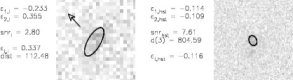
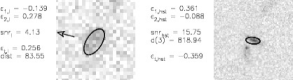
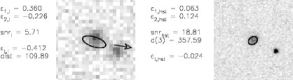
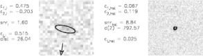
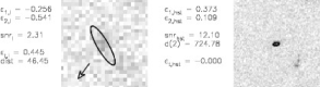
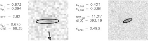
In Fig. 36, we present clippings of some of these galaxies from the two images to convey a visual impression on how they compare in the images and how the shape measurements relate to the image, especially for the ground-based image. We find that in the HST image, the measured ellipticity very well represents the shape of the object. This is to be expected as all these objects are detected with a high signal-to-noise ratio in the HST image. In the $I$-band image, these objects have a low signal-to-noise ratio and the ellipticity measurements only vaguely reflect the shape of the objects. About 10% of the objects are actually two or more objects which were not resolved in the ground-base image; for about 20% a nearby (though resolved) object seems to influence the ellipticity measurement. It is especially striking that for many, the ellipticity modulus $|\mbox{\boldmath${\rm\varepsilon}$\unboldmath}|$ is clearly overestimated.

B.5 Summary

We have shown that on average, ground-based and space-based ellipticity measurements agree very well. This justifies the assumption that weak lensing analyses based on ground-based data yield reliable results despite the smearing of object shapes by the Earth’s atmosphere.

For the HST ellipticities, we have found only little evidence that they might be biased due to the CTE problem, the PSF undersampling, or the anisotropy correction. This holds at least for bright objects, for fainter ones we have no possibility of comparison. Yet, previous analyses (Sect. A.2) have shown that these problems have little influence.

The fainter an object, the less reliable its shape measurement is (Fig. 25). The strong lensing signal seen in the ground-based data is caused mainly by faint objects, for which the ellipticity measurements in the two datasets deviate. In both datasets, there is a $M_{\rm ap}$ peak at the position of the dark clump, but the degree of tangential alignment is much stronger in the ground-based data. For many of these objects, the ellipticity modulus $|\mbox{\boldmath${\rm\varepsilon}$\unboldmath}|$ is overestimated in the ground-based measurements, and many of these seem to be accidentally tangentially aligned to the dark clump, thus causing a high $M_{\rm ap}$ signal.

References

- Bartelmann & Schneider (2001) Bartelmann, M. & Schneider, P. 2001, Phys. Rep., 340, 291
- Bertin & Arnouts (1996) Bertin, E. & Arnouts, S. 1996, A&AS, 117, 393
- Cavaliere & Fusco-Femiano (1978) Cavaliere, A. & Fusco-Femiano, R. 1978, A&A, 70, 677
- Dahle et al. (2003) Dahle, H., Pedersen, K., Lilje, P. B., Maddox, S. J., & Kaiser, N. 2003, ApJ, 591, 662
- Erben et al. (2003) Erben, T., Miralles, J. M., Clowe, D., et al. 2003, A&A, 410, 45
- Erben et al. (2001) Erben, T., van Waerbeke, L., Bertin, E., Mellier, Y., & Schneider, P. 2001, A&A, 366, 717
- Erben et al. (2000) Erben, T., van Waerbeke, L., Mellier, Y., et al. 2000, A&A, 355, 23
- Fruchter & Hook (2002) Fruchter, A. S. & Hook, R. N. 2002, PASP, 114, 144
- Gonzaga et al. (1998) Gonzaga, S., Biretta, J., Wiggs, M., et al. 1998, Instrument Science Report WFPC2 98-04,
- Gray et al. (2001) Gray, M. E., Ellis, R. S., Lewis, J. R., McMahon, R. G., & Firth, A. E. 2001, MNRAS, 325, 111
- Hamana et al. (2003) Hamana, T., Takada, M., & Yoshida, N. 2003, preprint astro-ph/0310607,
- Hoekstra et al. (1998) Hoekstra, H., Franx, M., Kuijken, K., & Squires, G. 1998, ApJ, 504, 636
- Kaiser & Squires (1993) Kaiser, N. & Squires, G. 1993, ApJ, 404, 441
- Kaiser et al. (1995) Kaiser, N., Squires, G., & Broadhurst, T. 1995, ApJ, 449, 460
- Miralles et al. (2002) Miralles, J. M., Erben, T., Hämmerle, H., et al. 2002, A&A, 388, 68
- Monet et al. (1998) Monet, D. B. A., Canzian, B., Dahn, C., et al. 1998, VizieR Online Data Catalog, 1252, 0
- Peacock (1999) Peacock, J. A. 1999, Cosmological physics (Cambridge University Press)
- Press et al. (1992) Press, W. H., Teukolsky, S. A., Vetterling, W. T., & Flannery, B. P. 1992, Numerical Recipes in C. The Art of Scientific Computing (Cambridge University Press, 2nd ed.)
- Riess (2000) Riess, A. 2000, Instrument Science Report WFPC2 00-04,
- Schneider (1996) Schneider, P. 1996, MNRAS, 283, 837
- Schneider et al. (1998) Schneider, P., Van Waerbeke, L., Jain, B., & Kruse, G. 1998, MNRAS, 296, 873
- Seitz & Schneider (2001) Seitz, S. & Schneider, P. 2001, A&A, 374, 740
- Umetsu & Futamase (2000) Umetsu, K. & Futamase, T. 2000, ApJ Lett., 539, L5
- Weinberg & Kamionkowski (2002) Weinberg, N. N. & Kamionkowski, M. 2002, MNRAS, 337, 1269