A Kinematic Model for Gamma Ray Bursts and Symmetric Jets

Abstract

Gamma ray bursts (GRB) occur at random points in the sky at cosmological distances. They emit intense $\gamma$ rays for a brief period. The spectrum then evolves through X–ray, optical region to possibly radio frequency. Though there are some models, the origin and time evolution of GRB are not well understood. Extragalactic radio sources also exhibit a baffling array of features that are poorly understood – the core emission in ultraviolet region, lobes in RF range, transient $\gamma$ and X–ray emissions etc. These two phenomena appear to be very different, but the time evolution of the core emission of radio sources is essentially the same as GRBs, though with different time constants. Here, we present a model unifying GRB and roughly symmetric radio sources based on light travel time effect and superluminality. The light travel time effect influences the way we perceive superluminal motion. An object, moving across our field of vision at superluminal speeds, will appear to us as two objects receding from a single point. The time evolution of the Doppler shifted radiation of such a superluminal object bears remarkable similarity to that of GRB and radio sources. Based on these observations, we derive a kinematic model for radio sources and GRBs and explain the puzzling features listed above. Furthermore, we predict the angular motion of the hotspots or knots in the jets and compare it to the proper motions reported in the literature (Biretta et al., 1999). We also compare the proper motion of a microquasar (Mirabel and Rodríguez, 1999) with our model and show excellent agreement. Our model also explains the observed blue/UV spectrum (and its time evolution) of the core region and the RF spectrum of the lobes, and why the radio sources appear to be associated with galactic nuclei. We make other quantitative predictions, which can be verified.

1 Introduction

Gamma Ray Bursts (GRBs) are short and intense flashes of $\gamma$ rays in the sky, lasting from a few milliseconds to several minutes (Piran, 2002). They are characterized by a prompt emission and an after glow at progressively softer energies. Thus, the initial $\gamma$ rays are promptly replaced by X–rays, light and even radio frequency waves. This softening of the spectrum has been known for quite some time (Mazets et al., 1982). More recently, an inverse decay of the peak energy with varying time constant has been used to empirically fit the observed time evolution of the peak energy (Ryde, 2005; Ryde et al., 2003). According to the fireball model, GRBs are produced when the energy of highly relativistic flows in stellar collapses are dissipated. There is an overall agreement with the observed phenomena, though the exact nature of the structure of the radiation jets from the collapsing stars is still an open question. In this article, we present a radically different model explaining the origin of GRBs, their occurrence in seemingly random points in the sky and the time evolution of their spectra.

Symmetric radio sources (galactic or extragalactic) may appear to be a completely distinct phenomenon. However, their cores show a similar time evolution in the peak energy, but with a much larger time constant. Other similarities have begun to attract attention in the recent years (Ghisellini, 2004). Due to observational constraints, the time evolution of the spectra of radio sources has not been studied in great detail, but one available example is the jet in 3C 273 (Jester et al., 2004), which shows a softening of the spectrum remarkably similar to GRBs. Our model unifies these two phenomena and make detailed predictions on the kinematics of such radio sources. We will first look at the apparent superluminal motion observed in some jets and its traditional explanation. We will then proceed to derive the model for explaining the kinematics such symmetric radio sources and apply it to GRBs.

Some of the radio sources show superluminal motion in the transverse direction. We can measure the transverse velocity of a celestial object almost directly using angular measurements, which are translated to a speed using its known (or estimated) distance from us. In the past few decades, scientists have observed (Biretta et al., 1999; Zensus, 1997) objects moving at apparent transverse velocities significantly higher than the speed of light. Some such superluminal objects were detected within our own galaxy (Mirabel and Rodríguez, 1994, 1999; Gisler, 1994; Fender et al., 1999). The special theory of relativity (SR) states that nothing can accelerate past the speed of light (Einstein, 1905). Thus a direct measurement of superluminal objects emanating from a single point (or a small region) would be a violation of SR at a fundamental level. However, before proclaiming a contradiction based on an apparent superluminal motion, one has to establish that it is not an artifact of the way one perceives transverse velocities. Rees (1966) offered an explanation why such apparent superluminal motion is not in disagreement with SR, even before the phenomenon was discovered. When an object travels at a high speed towards an observer, at a shallow angle with respect to his line of sight, it can appear to possess superluminal speeds. Thus, a measurement of superluminal transverse velocity by itself is not an evidence against SR. In this article, we re-examine this explanation (also known also as the light travel time effect.) We will show that the apparent symmetry of the extragalactic radio sources is inconsistent with this explanation.

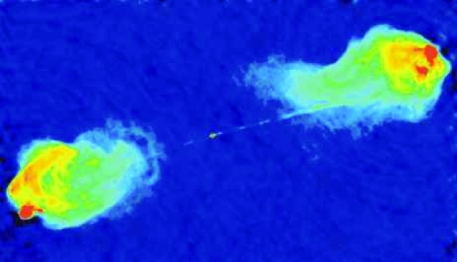
Figure 1: False color image of the radio jet and lobes in the hyperluminous radio galaxy Cygnus A. Red shows regions with the brightest radio emission, while blue shows regions of fainter emission. Image courtesy of NRAO/AUI.

Transverse superluminal motions are usually observed in quasars and microquasars. Different classes of such objects associated with Active Galactic Nuclei (AGN) were found in the last fifty years. Fig. 1 shows the radio galaxy Cygnus A (Perley et al., 1984) – one of the brightest radio objects. Many of its features are common to most extragalactic radio sources – the symmetric double lobes, an indication of a core, an appearance of jets feeding the lobes and the hotspots. Owsianik and Conway (1998) and Polatidis et al. (2002) have reported more detailed kinematic features, such as the proper motion of the hotspots in the lobes. We will show that our perception of an object crossing our field of vision at a constant superluminal speed is remarkably similar to a pair of symmetric hotspots departing from a fixed point with a decelerating rate of angular separation. We will make other quantitative predictions that can be verified, either from the current data or with dedicated experiments.

2 Traditional Explanation

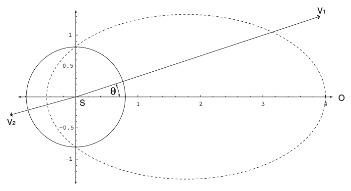
Figure 2: Illustration of the traditional explanation for the apparent superluminal motion. An object expanding at a speed $\beta=0.8$, starting from a single point S. The solid circle represents the boundary one second later. The observer is far away on the right hand side, O ($x\to\infty$). The dashed ellipse is the apparent boundary of the object, as seen by the observer.

First, we look at the traditional explanation of the apparent superluminal motion by the light travel time effect. Fig. 2 illustrates the explanation of apparent superluminal motion as described in the seminal paper by Rees (1966). In this figure, the object at S is expanding radially at a constant speed of $0.8c$, a highly relativistic speed. The part of the object expanding along the direction $V_{1}$, close to the line of sight of the observer, will appear to be traveling much faster. This will result in an apparent transverse velocity that can be superluminal.

The apparent speed $\beta^{\prime}$ of the object depends on the real speed $\beta$ and the angle between its direction of motion and the observer’s line of sight, $\theta$. As shown in Appendix A.1,

$$\beta^{\prime}\quad=\quad\frac{\beta}{1\,-\,\beta\cos\theta}$$ (1)

Fig. 2 is a representation of equation (1) as $\cos\theta$ is varied over its range. It is the locus of $\beta^{\prime}$ for a constant $\beta=0.8$, plotted against the angle $\,\theta$. The apparent speed is in complete agreement with what was predicted in 1966 (Fig. 1 in that article (Rees, 1966)).

For a narrow range of $\,\theta$, the transverse component of the apparent velocity ($\,\beta^{\prime}\sin\theta\,$) can appear superluminal. From equation (1), it is easy to find this range:

$$\frac{1-\sqrt{2\beta^{2}-1}}{2\beta}<\cos\theta<\frac{1+\sqrt{2\beta^{2}-1}}{2\beta}$$ (2)

Thus, for appropriate values of $\,\beta(>\frac{1}{\sqrt{2}})\,$ and $\,\theta\,$ (as given in equation (2)), the transverse velocity of an object can seem superluminal, even though the real speed is in conformity with the special theory of relativity.

While equations (1) and (2) explain the apparent transverse superluminal motion the difficulty arises in the recessional side. Along directions such as $V_{2}$ in Fig. 2, the apparent velocity is always smaller than the real velocity. The jets are believed to be emanating from the same AGN in opposite directions. Thus, if one jet is in the $\cos\theta$ range required for the apparent superluminal motion (similar to $V_{1}$), then the other jet has to be in a direction similar to $V_{2}$. Along this direction, the apparent speed is necessarily smaller than the real speed, due to the same light travel time effect that explains the apparent superluminal motion along $V_{1}$. Thus, the observed symmetry of these objects is inconsistent with the explanation based on the light travel time effect. Specifically, superluminality can never be observed in both the jets (which, indeed, has not been reported so far). However, there is significant evidence of near symmetric outflows (Laing et al., 1999) from a large number of objects similar to the radio source in Fig. 1.

One way out of this difficulty is to consider hypothetical superluminal speeds for the objects making up the apparent jets. Note that allowing superluminal speeds is not in direct contradiction with the special theory of relativity, which does not treat superluminality at all. The original derivation (Einstein, 1905) of the theory of coordinate transformation is based on the definition of simultaneity enforcing the constancy of the speed of light. The synchronization of clocks using light rays clearly cannot be done if the two frames are moving with respect to each other at superluminal speeds. All the ensuing equations apply only to subluminal speeds. It does not necessarily preclude the possibility of superluminal motion. However, an object starting from a fixed point and accelerating past the speed of light is clear violation of SR.

Another consequence of the traditional explanation of the apparent superluminal speed is that it is invariably associated with a blue shift. As given in equation (2), the apparent transverse superluminal speed can occur only in a narrow region of $\cos\theta$. In this region, the longitudinal component of the velocity is always towards the observer, leading to a blue shift. The existence of blue shift associated with all superluminal jets has not been confirmed experimentally. Quasars with redshifts have been observed with associated superluminal jets. Two examples are: quasars 3C 279 (Wehrle et al., 2001) with a redshift ${\mathbf{z}}=0.536$ and 3C 216 with ${\mathbf{z}}=0.67$ (Paragi et al., 2000). However, the Doppler shift of spectral lines applies only to normal matter, not if the jets are made up of plasma, as currently believed. Thus, the current model of jets, made up of plasma collimated by a magnetic field originating from an accretion disc, can accommodate the lack of blue shift.

3 A Model for Double–lobed Radio Sources GRBs

Accepting hypothetical superluminal speeds, we can clearly tackle the second consequence of the traditional explanation (namely, the necessity of blue shift along with apparent superluminal motion.) However, it is not clear how we perceive superluminal motion, because the light travel time effect will influence the way we perceive the kinematics. In this section, we will show that a single object moving superluminally, in a transverse direction across our field of vision, will look like two objects departing from a single point in a roughly symmetric fashion.

3.1 Symmetric Jets

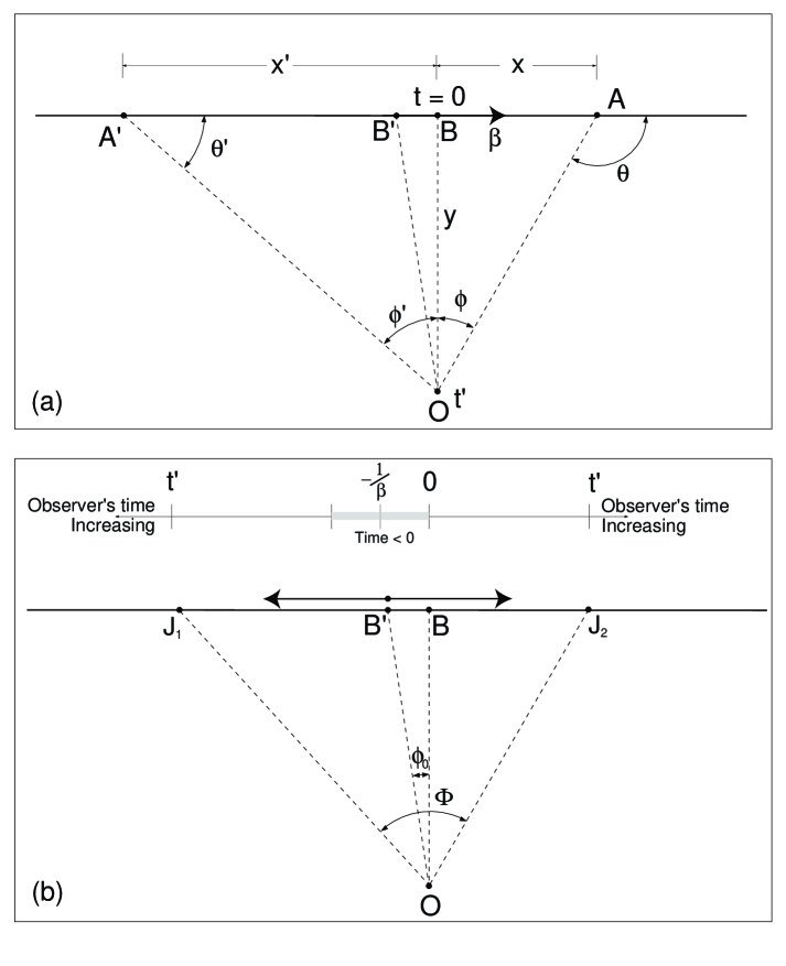
Figure 3: The top panel (a) shows an object flying along $A^{\prime}BA$ at a constant superluminal speed. The observer is at $O$. The object crosses $B$ (the point of closest approach to $O$) at time $t=0$. The bottom panel (b) shows how the object is perceived by the observer at $O$. It first appears at $B^{\prime}$, then splits into two. The two apparent objects seem to go away from each other (along $J_{1}$ and $J_{2}$) as shown.

Consider an object moving at a superluminal speed as shown in Fig. 3(a). The point of closest approach is $B$. At that point, the object is at a distance of $y$ from the observer at $O$. Since the speed is superluminal, the light emitted by the object at some point $B^{\prime}$ (before the point of closest approach $B$) reaches the observer before the light emitted at $A^{\prime}$. This gives an illusion of the object moving in the direction from $B^{\prime}$ to $A^{\prime}$, while in reality it is moving in the opposite direction.

We use the variable $t^{\prime}$ to denote the the observer’s time. Note that, by definition, the origin in the observer’s time axis is set when the object appears at $B$. $\phi$ is the observed angle with respect to the point of closest approach $B$. $\phi$ is defined as $\theta-\pi/2$ where $\theta$ is the angle between the object’s velocity and the observer’s line of sight. $\phi$ is negative for negative time $t$.

It is easy to derive the relation between $t^{\prime}$ and $\phi$. (See Appendix A.3 for the mathematical details.)

$$t^{\prime}=y\left(\frac{\tan\phi}{\beta}+\frac{1}{\cos\phi}-1\right)$$ (3)

Here, we have chosen units such that $c=1$, so that $y$ is also the time light takes to traverse $BO$. The observer’s time is measured with respect to $y$. i.e., $t^{\prime}=0$ when the light from the point of closest approach $B$ reaches the observer.

The actual plot of $\phi$ as a function of the observer’s time is given in Fig. 4. Note that for for subluminal speeds, there is only one angular position for any given $t^{\prime}$. The time axis scales with $y$. For subluminal objects, the observed angular position changes almost linearly with the observed time, while for superluminal objects, the change is parabolic.

Equation (3) can be approximated using a Taylor series expansion as:

$$t^{\prime}\approx y\left(\frac{\phi}{\beta}+\frac{\phi^{2}}{2}\right)$$ (4)

From the quadratic equation (4), one can easily see that the minimum value of $t^{\prime}$ is $t^{\prime}_{\rm min}=-y/2\beta^{2}$ and it occurs at $\phi_{0}=-1/\beta$. Thus, to the observer, the object first appears (as though out of nowhere) at the position $\phi_{0}$ at time $t^{\prime}_{\rm min}$. Then it appears to stretch and split, rapidly at first, and slowing down later. This apparent time evolution of the object is shown in Fig. 8, where it is compared to the microquasar GRS 1915+105 (Mirabel and Rodríguez, 1994; Fender et al., 1999).

The angular separation between the objects flying away from each other is:

$$\Phi=\frac{2}{\beta}\sqrt{1+\frac{2\beta^{2}}{y}t^{\prime}}=\frac{2}{\beta}\left(1+\beta\phi\right)$$ (5)

And the rate at which the separation occurs is:

$$\frac{d\Phi}{dt^{\prime}}=\sqrt{\frac{2}{yt_{\rm age}}}=\frac{2\beta}{y\left(1+\beta\phi\right)}$$ (6)

where $t_{\rm age}=t^{\prime}-t^{\prime}_{\rm min}$, the apparent age of the symmetric object.

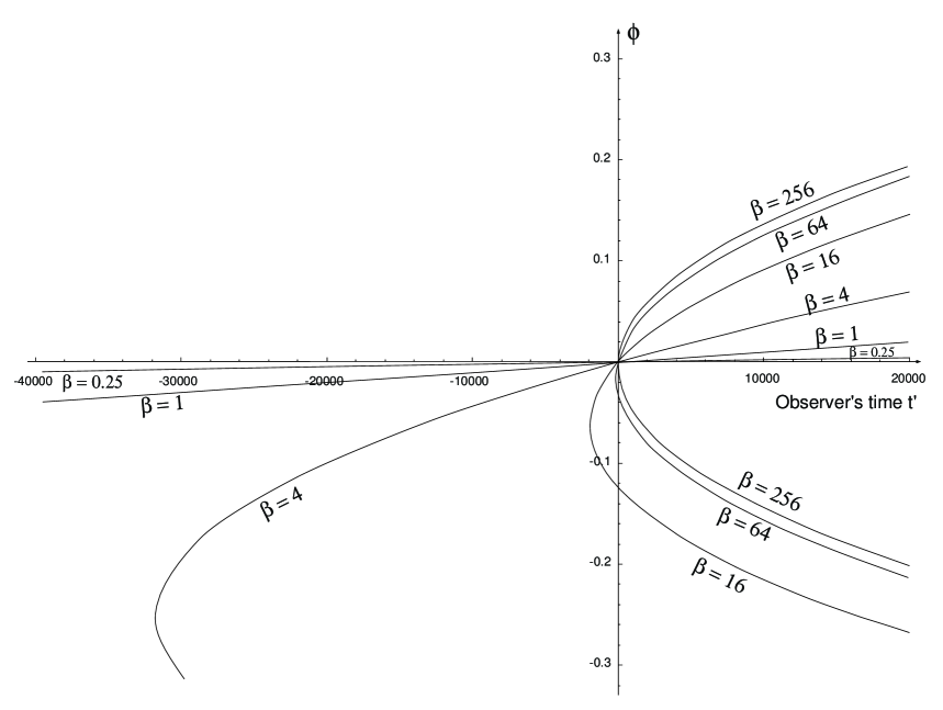
Figure 4: The apparent angular positions of an object traveling at different speeds at a distance $y$ of one million light years from us. The angular positions ($\phi$ in radians) are plotted against the observer’s time $t^{\prime}$ in years.

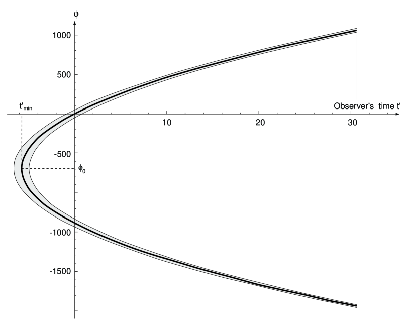
Figure 5: The apparent angular positions and sizes of an object traveling at $\beta=300$ at a distance $y$ of one million light years from us. The angular positions ($\phi$ in arc seconds) are plotted against the observer’s time $t^{\prime}$ in years. The shaded region represents the apparent angular spread of the object, with an assumed diameter of 500 light years.

This discussion shows that a single object moving across our field of vision at superluminal speed creates an illusion of an object appearing at a at a certain point in time, stretching and splitting and then moving away from each other. This time evolution is given in equation (3), and illustrated in the bottom panel of Fig. 3(b). Note that the apparent time $t^{\prime}$ is reversed with respect to the real time $t$ in the region $A^{\prime}$ to $B^{\prime}$. An event that happens near $B^{\prime}$ appears to happen before an event near $A^{\prime}$. Thus, the observer may see an apparent violation of causality, but it is just a part of the light travel time effect.

Fig. 5 shows the apparent width of a superluminal object as it evolves. The width decreases with time, along its direction of motion. (See Appendix A.5 for the mathematical details.) Thus, the appearance is that of two spherical objects appearing out of nowhere, moving away from each other, and slowly getting compressed into thinner and thinner ellipsoids and then almost disappearing.

If there are multiple objects, moving as a group, at roughly constant superluminal speed along the same direction, their appearance would be a series of objects appearing at the same angular position and moving away from each other sequentially, one after another. The apparent knot in one of the jets always has a corresponding knot in the other jet.

The calculation presented in this article is done in two dimensions. If we generalize to three dimensions, we can explain the precession observed in some systems. Imagine a cluster of objects, roughly in a planar configuration (like a spiral galaxy, for instance) moving together at superluminal speeds with respect to us. All these objects will have the points of closest approach to us in small angular region in our field of vision – this region is around the point of minimum distance between the plane and our position. If the cluster is rotating (at a slow rate compared to the superluminal linear motion), then the appearance to us would be the apparent jets changing directions as a function of time. The exact nature of the apparent precession depends on the spatial configuration of the cluster and its angular speed.

If we can measure the angle $\phi_{0}$ between the apparent core and the point of closest approach, we can directly estimate the real speed of the object $\beta$. We can clearly see the angular position of the core. However, the point of closest approach is not so obvious. We will show in the next section that the point of closest approach corresponds to zero redshift. (This is obvious intuitively, because at the the point of closest approach, the longitudinal component of the velocity is zero.) If this point ($\phi_{0}$) can be estimated accurately, then we can measure the speed directly, from the relation $\phi_{0}=-1/\beta$.

3.2 Redshifts of the Hotspots

In the previous section, we showed how a superluminal object can appear as two objects receding from a core. We can also work out the time evolution of the redshift of the two apparent objects (or hotspots). However, as relativistic Doppler shift equation is not defined for superluminal speeds, we need to work out the relationship between the redshift (${\mathbf{z}}$) and the speed ($\beta$) from first principles. This is easily done (see Appendix A.2 for the mathematical details):

$$1\,+\,{\mathbf{z}}\,=\,\left|1\,-\,\beta\cos\theta\right|\,=\,\left|1\,+\,\beta\sin\phi\right|$$ (7)

Since we allow superluminal speeds in our model of extragalactic radio sources, we can explain the radio frequency spectra of the hotspots as extremely red-shifted blackbody radiation. The $\beta$s involved in this explanation are typically very large, and we can approximate the redshift as:

$$1\,+\,{\mathbf{z}}\,\approx\,\left|\beta\phi\right|\,\approx\,\frac{\left|\beta\Phi\right|}{2}$$ (8)

Assuming the object to be a black body similar to the sun, we can predict the peak wavelength (defined as the wavelength at which the luminosity is a maximum) of the hotspots as:

$$\lambda_{\rm max}\,\approx\,(1+{\mathbf{z}})480nm\,\approx\,\frac{\left|\beta\Phi\right|}{2}480nm$$ (9)

where $\Phi$ is the angular separation between the two hotspots.

This shows that the peak RF wavelength increases linearly with the angular separation. If multiple hotspots can be located in a twin jet system, their peak wavelengths will depend only on their angular separation, in a linear fashion. The variation of the emission frequency from ultraviolet to RF as $\phi$ increases along the jet is clearly seen in the photometry of the jet in 3C 273 (Jester et al., 2004). Furthermore, if the measurement is done at a single radio frequency, intensity variation can be expected as the hotspot moves along the jet. Note that the limiting value of $|1+{\mathbf{z}}|$ is roughly $\beta$, which gives an indication of the hyperluminal speeds required to push the black body radiation to RF spectra.

3.3 Time Evolution of GRB spectra

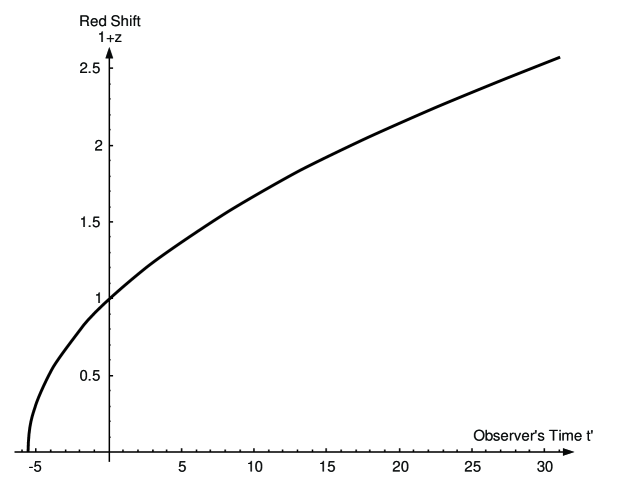
Figure 6: Time evolution of the redshift from a superluminal object. It shows the redshifts expected from an object moving at $\beta=300$ at a distance of ten million light years from us. The X axis is the observer’s time in years. (Since the X axis scales with time, it is also the redshift from an object at 116 light days – ten million light seconds – with the X axis representing $t^{\prime}$ in seconds.)

The evolution of redshift of the thermal spectrum of a hyperluminal object also holds the explanation for $\gamma$ ray bursts. Since we know the dependence of the observer’s time $t^{\prime}$ and the redshift $1+{\mathbf{z}}$ on the real time $t$, we can plot one against the other parametrically. (See Appendix A.4.) Fig. 6 shows the variation of redshift as a function of the observer’s time ($t^{\prime}$). It shows that the observed spectra of a superluminal object is expected to start at the observer’s time $t^{\prime}_{\rm min}$ with heavy (infinite) blue shift. The spectrum of the object rapidly softens and soon evolves to zero redshift and on to higher values. The rate of softening depending on the its speed and distance from us, which is the only difference between GRBs and symmetric jets (or radio sources) in this model. Note that to the observer, before $t^{\prime}_{\rm min}$, there is no object. In other words, there is a definite point in the observer’s time when the GRB is “born”, with no indication of its impending birth before that time. This birth does not correspond to any cataclysmic event (as would be required in the collapsar/hypernova or the “fireball” model) at the distant object. It is just an artifact of our perception.

There are two solutions for ${\mathbf{z}}$ for any given $t^{\prime}$, corresponding to the apparent objects at the two different positions. However, as shown in Appendix A.4, they are nearly identical (especially for small $\phi$). For $t^{\prime}<0$, there is a strong blue shift, which explains the observed, transient hard X–ray spectra of some of the symmetric jets. Donley et al. (2002) have a recent survey of such data, though the currently favored explanation for such transient emissions is a stellar tidal disruption scenario. The small difference between the redshifts of the two apparent objects may explain the double peak structure observed in the spectral data of some of the AGNs (Eracleous and Halpern, 2003).

Note that the X axis in Fig. 6 scales with time. We have plotted an object with $\beta=300$ and $y=$ ten million light years, with X axis is $t^{\prime}$ in years. It is also the variation of $1+{\mathbf{z}}$ for an object at $y=$ ten million light seconds (or 116 light days) with X axis in seconds. The former corresponds to a symmetric jets and the latter to a GRB. Thus, for a GRB, the spectral evolution takes place at a much faster pace. Clearly, different combinations of $\beta$ and $y$ can be fitted to describe different GRB spectral evolutions.

We can also eliminate $t$ and study the time evolution of $1+{\mathbf{z}}$. In order to make the algebra more manageable, we define $\tau=y/\beta$, a characteristic time scale for the GRB (or the radio source). This is the time the object would take to reach us, if it were coming directly toward us. We also define the age of the GRB (or radio source) as $=t_{\rm age}=t^{\prime}-t^{\prime}_{\rm min}$. This is just the observer’s time ($t^{\prime}$) shifted by the time at which the object first appears to him ($t^{\prime}_{\rm min}$). With these notations (and for small values $t$), it is possible to write the time dependence of ${\mathbf{z}}$ as:

$$1+{\mathbf{z}}=\left|{1+\frac{{\beta^{2}\left({-\tau\pm\sqrt{2\beta t_{{\rm age}}}}\right)}}{{\beta t_{{\rm age}}+\tau/2\mp\sqrt{2\beta t_{{\rm age}}}+\beta^{2}\tau}}}\right|$$ (10)

for small values of $t\ll\tau$. (The derivation of this equation can be found in Appendix A.4.)

Since the peak energy of the spectrum is inversely proportional to the redshift, it can be written as

$$E_{\rm pk}(t_{{\rm age}})=\frac{E_{\rm pk}(t_{\rm min})}{1+C_{1}\,\sqrt{\frac{t_{{\rm age}}}{\tau}}+C_{2}\,\frac{t_{{\rm age}}}{\tau}}$$ (11)

where $C_{1}$ and $C_{2}$ are coefficients to be estimated by the Taylor series expansion of equation (10) or by fitting.

The evolution of the peak energy ($E_{\rm pk}(t)$) has been empirically modeled (Ryde and Svensson, 2000) as:

$$E_{\rm pk}(t)=\frac{E_{\rm pk,0}}{(1+t/\tau)^{\delta}}$$ (12)

where $t$ is the time elapsed after the onset ($=t_{\rm age}$ in our notation), $\tau$ is a time constant and $\delta$ is the hardness intensity correlation (HIC). Out of the seven fitted values of $\delta$ from Ryde and Svensson (2000), one can calculate the average as $\delta=1.038\pm 0.014$, with the individual values ranging from $0.4$ to $1.1$. A fit to equation (11) may give better results, but within the statistics, it may not rule out or validate either model. Furthermore, it is not an easy fit, because there are too many unknowns. However, it is easy to see that the shape of equations (11) and (12) are remarkably similar.

3.4 Summary of Predictions

Some of the different quantitative predictions of the model are recapitulated here. These are predictions that are relatively easy to verify with existing data.

• The appearance of a single object moving across our field of vision at superluminal speed is that of an object appearing at a point, splitting and moving away in opposite directions.

• The core will always have a fixed angular position.

• The new superluminal knots appearing in the jets will always appear in pairs.

• The two apparent objects will shrink monotonically. As the knots move away from the core, they become thinner and thinner ellipsoids, contracting along the direction of motion while the transverse size remains roughly constant.

• The separation speed is very high in the beginning, but it slows down parabolically with time.

• The hotspots have almost identical RF spectra (and redshifts).

• The RF wavelength at which the luminosity of the hotspots is a maximum increases linearly with the angular separation between them.

• Close to the core, the the spectrum is heavily blue shifted. Thus, the object can be a strong X–ray or even $\gamma$ ray source for a brief period of time. After that, the spectrum moves through optical to RF region.

• Since GRBs and symmetric jets are essentially the same cosmological phenomenon in this model, at least some of the GRBs will evolve to be symmetric jets with possible superluminal transverse speeds.

A clear indication of a movement in the core’s angular position, or a superluminal knot appearing without a counterpart in the opposite jet will be strong evidence against our model based on superluminality. On the other hand, a clear measurement of apparent superluminal motion in both the jets (not reported so far) will provide a convincing indication that the conventional explanation is inadequate.

3.5 Comparison to Measurements

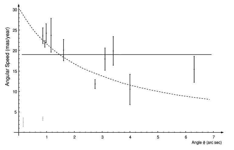
Figure 7: The angular speed of M87 (as a function of the feature angle $\phi$) fitted against our model. The solid line constrains the distance of closest approach to the estimated distance of M87 – 52 million light years, giving a $\beta=4.8$. The dotted line is a free fit giving $\beta=84\,000$.

Biretta et al. (1999) have reported proper motion in one of the jets of M87 as a function of the angle ($\phi$) between the apparent core and the feature points. M87 is estimated to be at about 52 million light years away from us, which gives us the value of $y$. In equation (6), we have the apparent angular speed ($d\Phi/dt^{\prime}$) as a function of $\phi$. Making the reasonable approximation $\Phi\approx 2\phi$, we can fit these data to our equation. The result is shown in Fig. 7. The fit gives a value $\beta=4.8$. A cluster of objects flying across our field of vision, about five times faster than light and at a distance of 52 million light years, will look like two jets moving away from each other at roughly 38 mas/year. If one of the two jets is hidden for some reason, the appearance will be a single jet of objects moving away from a point with an angular speed of about 19 mas/year. Note that we exclude the first two points from the fit. In this region close to the core, the appearance of new objects makes it difficult to track the features.

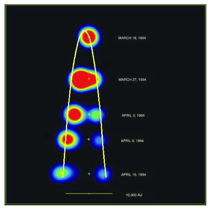
Figure 8: Fit of our model to the time evolution measurements of GRS1915+105. The yellow curve overlaid corresponds to our perception of a single superluminal object, traveling at $\beta=3\,000$ across our field of vision.

A much better fit can be obtained if we were to let the distance $y$ also float. The resulting $\beta$ of about 90 000 may explain the spectra of the hotspots. While the estimated $\beta$ may look excessive, once superluminal motion is allowed, there is no a priori reason why it should not take any value at all. Fig. 8 shows another comparison of our model to the data available in the literature. Here, the time evolution of the microquasar GRS 1915+105 (Mirabel and Rodríguez, 1994; Fender et al., 1999) is fitted to our model of a single superluminal object. The deceleration of relativistic jets (one of the predictions from our model) has been observed in the Microquasar XTE J1550-564 (Corbel et al., 2002), though it is currently believed to be an effect similar to frictional drag.

AGNs are known to have intensely blue or ultraviolet core, not easily explained by thermal models. But, this is an expected feature in our model. As seen in equation (9), the core (where $\Phi\to 0$) must have a highly blue shifted spectrum. A clear evolution of emission frequency from ultraviolet to RF is seen in the photometry of the jet in 3C 273 (Jester et al., 2004). The spectrum shifts from lower wavelength to higher as a function of the angular distance from the core, strikingly consistent with our prediction.

This shifting of peak frequency can be seen at a much larger scale in Fig. 1. The size of the optical core is about a tenth of the angular separation between the hotspots. If we model Cygnus A as a collection of objects moving together at superluminal speeds, the core region would have emissions in the $\gamma$, X-ray, UV or optical region. As we move away towards the hotspots, the peak frequency would continuously shift to RF. This behavior is indeed reported (Bach et al., 2004) recently. This also partially explains why extragalactic radio sources seem to be associated with galactic nuclei, instead of appearing randomly in the sky. A large collection of objects moving together (a large spiral galaxy, viewed from the side, for instance) superluminally gives the impression of a smaller stationary object with optical emission. The apparent object is likely to appear elongated along the direction of motion (with the major axis along the direction of the jets), with RF lobes appearing symmetrically farther away from the core. If the motion is not along a linear trajectory, we may see curved jets.

4 Conclusions

In this article, we presented a unified model for Gamma Ray Bursts and jet like radio sources based on bulk superluminal motion. We showed that a single superluminal object flying across our field of vision would appear to us as the symmetric separation of two objects from a fixed core. Using this fact as the model for symmetric jets and GRBs, we explain their kinematic features quantitatively. In particular, we showed that the angle of separation of the hotspots is parabolic in time, and the redshifts of the two hotspots are almost identical to each other. Even the fact that the spectra of the hotspots are in the radio frequency region is explained by assuming hyperluminal motion and the consequent redshift of the blackbody radiation. The time evolution of the black body radiation of a superluminal object is extremely consistent with the softening of the spectra observed in GRBs and symmetric jets. In addition, our model explains why there is significant blue shift at the core regions of radio sources, why radio sources seem to associated with optical galaxies and why GRBs appear at random points with no advance indication of their impending appearance.

The currently favored models for these phenomena require either cataclysmic events (explosions and shock waves in the fireball model of GRBs) or space singularities (black hole accretion for jets). GRBs are observed at a rate of one per day, and are expected to be observed much more frequently with the Swift mission. The number of observed jet like sources observed also is on the increase. This makes the explanations based on singularities and explosions less appealing. Our model presents a more attractive option based on how we perceive superluminal motion. However, it does not address the energetics issues – the origin of superluminality.

We presented a set of predictions and compared them to existing data. The features such as the blueness of the core, symmetry of the lobes, the transient $\gamma$ and X-Ray bursts, the measured evolution of the spectra along the jet all find natural and simple explanations in this model. Note that our model does not preclude plasma jets that may be related to space-time singularities or other massive objects and the associated accretion discs. The conventional explanation of the apparent superluminal motion in asymmetric jets (e.g., quasar 3C 279 Wehrle et al. (2001)) also stands. In fact, our model is just a generalization of the conventional explanation.

We also explored the full implications of the traditional explanation for the apparent superluminal motion observed in certain quasars and microquasars. The equation that explains the apparent superluminal speeds predicts that objects receding from us should appear to be moving slower. Thus, in a symmetric radio sources where it is observed, the superluminal motion can appear only in one of the jets. The observed symmetry of these extragalactic radio sources (even subluminal ones) is incompatible with the explanation. Another consequence is that an apparent superluminal motion (if the moving objects are composed of normal matter rather than plasma) must always show a blue shift, a redshifted object can never be superluminal. In our model, the requirement that an apparent superluminal motion be associated with a blue shift does not apply any more. Furthermore, the jets are expected to be fairly symmetric.

We argued that superluminal motion is not inconsistent with the special theory of relativity, which just does not deal with it. Acceptance of superluminality has far-reaching consequences in other long established notions of our universe. (See Appendix B for an incomplete list.) The description of extragalactic (or galactic) radio sources in terms of superluminal motion has a direct impact on our understanding of black holes.

Appendix

Appendix A Mathematical Details

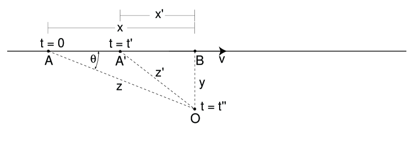
Figure 9: The object is flying along $AB$, the observer is at $O$. The object crosses $A$ at time $t=0$. It reaches $A^{\prime}$ at time $t=t^{\prime}$. A photon emitted at $A$ reaches $O$ at time $t=t_{0}$, and a photon emitted at $A^{\prime}$ reaches $O$ at time $t=t^{\prime\prime}$.

A.1 Velocity Profile of an Expanding Object

In this section, we derive the ellipse in Fig. 2 from first principles. In Fig. 9, there is an observer at $O$. An object is flying by at a high speed $v=\beta c$ along the horizontal line $AB$. With no loss of generality, we can assume that $t=0$ when the object is at $A$. It passes $A^{\prime}$ at time $t^{\prime}$. The photon emitted at time $t=0$ reaches the observer at time $t=t_{0}$, and the photon emitted at $A^{\prime}$ (at time $t=t^{\prime}$) reaches him at time $t=t^{\prime\prime}$. The angle between the object’s velocity at $A$ and the observer’s line of sight is $\theta$. We have the Pythagoras equations:

$$z^{2}\, = \,x^{2}\,+\,y^{2}$$ (13)

$$z^{\prime 2}\, = \,x^{\prime 2}\,+\,y^{2}$$ (14)

$$\Rightarrow\qquad\frac{x+x^{\prime}}{z+z^{\prime}} \,=\, \frac{z-z^{\prime}}{x-x^{\prime}}$$ (15)

If we assume that $x$ and $z$ (distances at time $t_{0}$) are not very different from $x^{\prime}$ and $z^{\prime}$ respectively (distances at time $t^{\prime}$), we can write,

$$\cos\theta=\frac{x}{z}\approx\frac{x+x^{\prime}}{z+z^{\prime}}=\frac{z-z^{\prime}}{x-x^{\prime}}$$ (16)

We define the real speed of the object as:

$$v\,=\,\beta\,c\,=\,\frac{x\,-\,x^{\prime}}{t^{\prime}}$$ (17)

But the speed it appears to have will depend on when the observer senses the object at $A$ and $A^{\prime}$. The apparent speed of the object is:

$$v^{\prime}\,=\,\beta^{\prime}\,c\,=\,\frac{x\,-\,x^{\prime}}{t^{\prime\prime}\,-\,t_{0}}$$ (18)

Thus,

$$\frac{\beta}{\beta^{\prime}}\, = \,\frac{t^{\prime\prime}-t_{0}}{t^{\prime}}$$ (19)

$$= \,1+\frac{z^{\prime}-z}{ct^{\prime}}$$ (20)

$$= \,1-\frac{x-x^{\prime}}{ct^{\prime}}\cos\theta$$ (21)

$$= \,1-\beta\cos\theta$$ (22)

which gives,

$$\beta^{\prime}\quad=\quad\frac{\beta}{1\,-\,\beta\cos\theta}$$ (23)

Fig. 2 is the locus of $\beta^{\prime}$ for a constant $\beta=0.8$, plotted against the angle $\,\theta$.

A.2 Superluminal Redshift

Redshift (${\mathbf{z}}$) defined as:

$$1\,+\,{\mathbf{z}}\,=\,\frac{\lambda^{\prime}}{\lambda}$$ (24)

where $\lambda^{\prime}$ is the measured wavelength and $\lambda$ is the known wavelength. In Fig. 9, the number of wave cycles created in time $t^{\prime}$ between $A$ and $A^{\prime}$ is the same as the number of wave cycles sensed at $O$ between $t_{0}$ and $t^{\prime\prime}$. Substituting the values, we get:

$$\frac{t^{\prime}\,c}{\lambda}\,=\,{\frac{(t^{\prime\prime}\,-\,t_{0})\,c}{\lambda^{\prime}}}$$ (25)

Using the definitions of the real and apparent speeds, it is easy to get

$$\frac{\lambda^{\prime}}{\lambda}\,=\,\frac{\beta}{\beta^{\prime}}$$ (26)

Using the relationship between the real speed $\beta$ and the apparent speed $\beta^{\prime}$ (equation (23)), we get

$$1\,+\,{\mathbf{z}}\,=\,\frac{1}{1\,+\,\beta^{\prime}\cos\theta}\,=\,1\,-\,\beta\cos\theta$$ (27)

As expected, ${\mathbf{z}}$ depends on the longitudinal component of the velocity of the object. Since we allow superluminal speeds in this calculation, we need to generalize this equation for ${\mathbf{z}}$ noting that the ratio of wavelengths is positive. Taking this into account, we get:

$$1\,+\,{\mathbf{z}}\,=\,\left|\frac{1}{1\,+\,\beta^{\prime}\cos\theta}\right|\,=\,\left|1\,-\,\beta\cos\theta\right|$$ (28)

A.3 Kinematics of Superluminal Objects

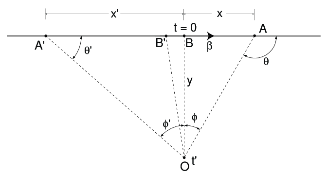
Figure 10: An object flying along $A^{\prime}BA$ at a constant superluminal speed. The observer is at $O$. The object crosses $B$ (the point of closest approach to $O$) at time $t=0$.

The derivation of the kinematics is based on Fig. 10. Here, an object is moving at a superluminal speed along $A^{\prime}BA$. At the point of closest approach, $B$, the object is a distance of $y$ from the observer at $O$. Since the speed is superluminal, the light emitted by the object at some point $B^{\prime}$ (before the point of closest approach $B$) reaches the observer before the light emitted at $A^{\prime}$. This gives an illusion of the object moving in the direction from $B^{\prime}$ to $A^{\prime}$, while in reality it is moving from $A^{\prime}$ to $B^{\prime}$. $\phi$ is the observed angle with respect to the point of closest approach $B$. $\phi$ is defined as $\theta-\pi/2$ where $\theta$ is the angle between the object’s velocity and the observer’s line of sight. $\phi$ is negative for negative time $t$.

We choose units such that $c=1$, in order to make algebra simpler. $t^{\prime}$ denotes the the observer’s time. Note that, by definition, the origin in the observer’s time, $t^{\prime}$ is set when the object appears at $B$.

The real position of the object at any time $t$ is:

$$x=y\tan\phi=\beta t$$ (29)

A photon emitted at $t$ will reach $O$ after traversing the hypotenuse. A photon emitted at $B$ will reach the observer at $t=y$, since we have chosen $c=1$. If we define the observer’s time $t^{\prime}$ such that the time of arrival is $t=t^{\prime}+y$, then we have:

$$t^{\prime}=t+\frac{y}{\cos\phi}-y$$ (30)

which gives the relation between $t^{\prime}$ and $\phi$.

$$t^{\prime}=y\left(\frac{\tan\phi}{\beta}+\frac{1}{\cos\phi}-1\right)$$ (31)

Expanding the equation for $t^{\prime}$ to second order, we get:

$$t^{\prime}=y\left(\frac{\phi}{\beta}+\frac{\phi^{2}}{2}\right)$$ (32)

The minimum value of $t^{\prime}$ occurs at $\phi_{0}=-1/\beta$ and it is $t^{\prime}_{\rm min}=-y/2\beta^{2}$. To the observer, the object first appears at the position $\phi=-1/\beta$. Then it appears to stretch and split, rapidly at first, and slowing down later.

The quadratic equation (32) can be recast as:

$$1+\frac{2\beta^{2}}{y}t^{\prime}=\left(1+\beta\phi\right)^{2}$$ (33)

which will be more useful later in the derivation.

The angular separation between the objects flying away from each other is the difference between the roots of the quadratic equation (32):

$$\Phi\, = \,\phi_{1}-\phi_{2}$$ (34)

$$= \,\frac{2}{\beta}\sqrt{1+\frac{2\beta^{2}}{y}t^{\prime}}$$ (35)

$$= \,\frac{2}{\beta}\left(1+\beta\phi\right)$$ (36)

making use of equation (33).

Thus, we have the angular separation either in terms of the observer’s time ($\Phi(t^{\prime})$) or the angular position of the object ($\Phi(\phi)$) as illustrated in Figure 11.

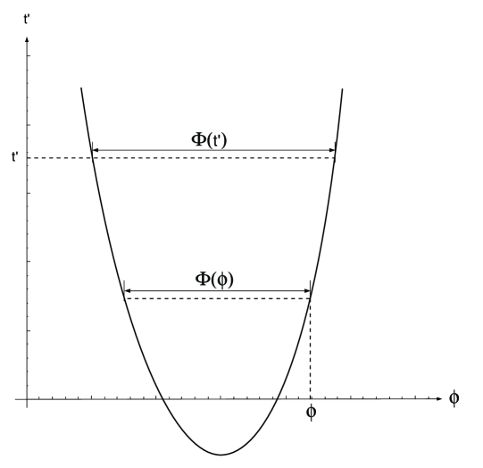
Figure 11: Illustration of how the angular separation is expressed either in terms of the observer’s time ($\Phi(t^{\prime})$) or the angular position of the object ($\Phi(\phi)$)

The rate at which the angular separation occurs is:

$$\frac{d\Phi}{dt^{\prime}}\, = \,\frac{2\beta}{y\sqrt{1+\frac{2\beta^{2}}{y}t^{\prime}}}$$ (37)

$$= \,\frac{2\beta}{y\left(1+\beta\phi\right)}$$ (38)

Again, making use of equation (33).

Defining the apparent age of the radio source $t_{\rm age}=t^{\prime}-t^{\prime}_{\rm min}$ and knowing $t^{\prime}_{\rm min}=-y/2\beta^{2}$, we can write:

$$\frac{d\Phi}{dt^{\prime}}\, = \,\frac{2\beta}{y\sqrt{1+\frac{2\beta^{2}}{y}t^{\prime}}}$$ (39)

$$= \,\frac{2\beta}{y\sqrt{1-\frac{t^{\prime}}{t_{\rm min}}}}$$ (40)

$$= \,\sqrt{\frac{-t_{\rm min}}{t^{\prime}-t_{\rm min}}}$$ (41)

$$= \,\sqrt{\frac{2}{yt_{\rm age}}}$$ (42)

A.4 Time Evolution of the Redshift

As shown before in equation (28), the redshift ${\mathbf{z}}$ depends on the real speed $\beta$ as:

$$1\,+\,{\mathbf{z}}\,=\,\left|1\,-\,\beta\cos\theta\right|\,=\,\left|1\,+\,\beta\sin\phi\right|$$ (43)

For any given time ($t^{\prime}$) for the observer, there are two solutions for $\phi$ and ${\mathbf{z}}$. $\phi_{1}$ and $\phi_{2}$ lie on either side of $\phi_{0}=1/\beta$. For $\sin\phi>-1/\beta$, we get

$$1+{\mathbf{z}}_{2}=1+\beta\sin\phi_{1}$$ (44)

and for $\sin\phi<-1/\beta$,

$$1+{\mathbf{z}}_{1}=-1-\beta\sin\phi_{2}$$ (45)

Thus, we get the difference in the redshift between the two hotspots as:

$$\Delta{\mathbf{z}}\approx 2+\beta(\phi_{1}+\phi_{2})$$ (46)

We also have the mean of the solutions of the quadratic ($\phi_{1}$ and $\phi_{2}$) equal to the position of the minimum ($\phi_{0}$):

$$\frac{\phi_{1}+\phi_{2}}{2}=-\frac{1}{\beta}$$ (47)

Thus $\phi_{1}+\phi_{2}=-2/\beta$ and hence $\Delta{\mathbf{z}}=0$. The two hotspots will have identical redshifts, if terms of $\phi^{3}$ and above are ignored.

As shown before (see equation (43)), the redshift ${\mathbf{z}}$ depends on the real speed $\beta$ as:

$$1\,+\,{\mathbf{z}}\,=\,\left|1\,+\,\beta\sin\phi\right|\,=\,\left|1\,+\,\frac{\beta^{2}t}{\sqrt{\beta^{2}t^{2}+y^{2}}}\right|$$ (48)

Since we know ${\mathbf{z}}$ and $t^{\prime}$ functions of $t$, we can plot their inter-dependence parametrically. This is shown in Fig. 6.

It is also possible to eliminate $t$ and derive the dependence of $1+{\mathbf{z}}$ on the apparent age of the object under consideration, $t_{\rm age}=t^{\prime}-t_{\rm min}$. In order to do this, we first define a time constant $\tau=y/\beta$. This is the time the object would take to reach us, if it were flying directly toward us.

First, let’s get an expression for $t/\tau$:

$$t^{\prime}\, = \,t+\sqrt{\beta^{2}t^{2}+y^{2}}-y$$ (49)

$$= \,t+\beta\tau\sqrt{1+\frac{{t^{2}}}{{\tau^{2}}}}-\beta\tau$$ (50)

$$\approx \,t+\frac{{\beta t^{2}}}{{2\tau}}$$ (51)

$$\Rightarrow\frac{t}{\tau}\, = \,\frac{{-1\pm\sqrt{1+\frac{{2\beta t_{\rm age}}}{\tau}}}}{\beta}$$ (52)

Note that this is valid only for $t\ll\tau$.

Now we collect the terms in $t/\tau$ in the equation for $1+{\mathbf{z}}$:

$$t^{\prime}\, = \,t+\sqrt{\beta^{2}t^{2}+y^{2}}-y$$ (53)

$$\Rightarrow\sqrt{\beta^{2}t^{2}+y^{2}}\, = \,t^{\prime}-t+y$$ (54)

$$1+z\, = \,\left|{1+\frac{{\beta^{2}t}}{{\sqrt{\beta^{2}t^{2}+y^{2}}}}}\right|$$ (55)

$$= \,\left|{1+\frac{{\beta^{2}t}}{{t^{\prime}-t+y}}}\right|$$ (56)

$$= \,\left|{1+\frac{{\beta^{2}\frac{t}{\tau}}}{{\frac{{t_{{\rm age}}}}{\tau}-\frac{1}{{2\beta}}-\frac{t}{\tau}+\beta}}}\right|$$ (57)

As expected, the time variables always appear as ratios like $t/\tau$, giving confidence that our choice of the characteristic time scale is probably right.

Finally, we can substitute $t/\tau$ from equation (52) in equation (57) to obtain:

$$1+{\mathbf{z}}=\left|{1+\frac{{\beta^{2}\left({-\tau\pm\sqrt{2\beta t_{{\rm age}}}}\right)}}{{\beta t_{{\rm age}}+\tau/2\mp\sqrt{2\beta t_{{\rm age}}}+\beta^{2}\tau}}}\right|$$ (58)

A.5 Time Evolution of the Object Size

Fig. 5 shows the apparent positions ($\phi$) and the size of the superluminal object as the observer sees it, as a function of the observer’s time ($t^{\prime}$). Fig. 6 is a similar time evolution of the redshift (${\mathbf{z}}$). In this section, we describe how these two plots are created. It is easiest to express the quantities parametrically as a function of the real time $t$. Referring to Fig. 10, we write,

$$x \,=\, \beta t$$ (59)

$$t^{\prime} \,=\, t+\sqrt{\beta^{2}t^{2}+y^{2}}-y$$ (60)

$$\sin\phi \,=\, \frac{x}{\sqrt{x^{2}+y^{2}}}=\frac{\beta t}{\sqrt{\beta^{2}t^{2}+y^{2}}}$$ (61)

The solid parabola in Fig. 5 is $\phi$ vs. $t^{\prime}$ from these equations as $t$ is varied between $-40$ and $20$ years, with $y=1\,000\,000$ light years and $\beta=300$.

In order to get the variation of the size of the object (the shaded region in Fig. 5), we assume a diameter $d=500$ light years.

$$t^{\prime}_{\pm}\, = \,t+\sqrt{\left(\beta t\pm\frac{d}{2}\right)^{2}+y^{2}}-y$$ (62)

$$\sin\phi_{\pm}\, = \,\frac{\beta t\pm\frac{d}{2}}{\sqrt{\left(\beta t\pm\frac{d}{2}\right)^{2}+y^{2}}}$$ (63)

The boundaries of the shaded region are given by $\phi_{+}$ vs. $t^{\prime}_{+}$ and $\phi_{-}$ vs. $t^{\prime}_{-}$.

Appendix B Perceived Properties of the Universe

It can be shown that the apparent expansion of the universe at strictly subluminal speed is also an artifact of our perception of superluminal motion. The apparent recessional speed is the longitudinal component of $\beta^{\prime}$ is $\beta^{\prime}_{\parallel}=\beta^{\prime}\cos\theta$. From equation (1), we can see that

$$\lim_{\beta\to\pm\infty}\beta^{\prime}_{\parallel}\,=\,-1$$ (64)

The apparent recessional speed (which can be measured using redshifts) tends to $c$ (or, $\,\beta^{\prime}_{\parallel}\,\to\,-1$), when the real speed is highly superluminal. This limit is independent of the actual direction of motion of the object $\theta$. Thus, whether a superluminal object is receding or approaching (or, in fact, moving in any other direction), the appearance from our perspective would be an object receding roughly at the speed of light. This appearance of all (possibly superluminal) objects receding from us at strictly subluminal speeds is an artifact of our perception, rather than the true nature of the universe.

Note that the equation for $1+{\mathbf{z}}$ has a limiting value of the real speed $|1+\beta|$ as large angles $\phi$. Thus, if we picture our universe as a large number of superluminal or hyperluminal objects moving around in random directions, there will be a significant amount of low frequency isotropic electromagnetic radiation. The spectrum of this cosmic microwave background can be directly translated to a velocity distribution of the celestial objects. The spatial asymmetry in the background radiation corresponds to a temporal evolution of the superluminal objects. Thus, even the cosmic microwave background radiation (considered one of the strongest arguments for the big bang model) can be accommodated in our model.

While working out various kinematic properties of superluminal objects, we noted that there is an apparent violation of causality when the superluminal object is approaching us. We also saw that a receding object can never appear to be going faster than the speed of light, even if the real speed is superluminal. For a receding object (even subluminal ones), there is a contraction of object size along the direction of motion and a time dilation effect. All these effects are due to the light travel time effect, but are remarkably similar to the theory of special relativity. However, the light travel time effect is currently assumed to apply on a space–time that obeys SR. It may be that there is a deeper structure to the space–time, of which SR is only our perception, filtered through the light travel time effect. By treating light travel time effect as an optical illusion to be applied on an SR–like space–time, we may be double counting the effects.

References

- Bach et al. (2004) Bach, U., Krichbaum, T. P., Middelberg, E., Kadler, M., Alef, W., Witzel, A., Zensus, J. A., Sep. 2004. Spectral Properties of the Core and the VLBI-Jets of Cygnus A. In: Bachiller, R., Colomer, F., Desmurs, J.F.and de Vicente, P. (Eds.), Proceedings of the 7th European VLBI Network Symposium.
- Biretta et al. (1999) Biretta, J. A., Sparks, W. B., Macchetto, F., Aug. 1999. Hubble space telescope observations of superluminal motion in the M87 jet. ApJ 520, 621–626.
- Corbel et al. (2002) Corbel, S., Fender, R. P., Tzioumis, A. K., Tomsick, J. A., Orosz, J. A., Miller, J. M., Wijnands, R., Kaaret, P., Oct. 2002. Large-Scale, Decelerating, Relativistic X-ray Jets from the Microquasar XTE J1550-564. Science 298, 196–198.
- Donley et al. (2002) Donley, J. L., Brandt, W. N., Eracleous, M. C., Boller, T., 2002. Large-Amplitude X-ray Outbursts from Galactic Nuclei: A Systematic Survey Using ROSAT Archival Data. AJ 124, 1308.
- Einstein (1905) Einstein, A., 1905. Zur Elektrodynamik bewegter Körper. (On the electrodynamics of moving bodies). Annalen der Physik 17, 891.
- Eracleous and Halpern (2003) Eracleous, M., Halpern, J., Dec. 2003. Completion of a Survey and Detailed Study of Double-Peaked Emission Lines in Radio-Loud AGNs. ApJ 599, 886–908.
- Fender et al. (1999) Fender, R. P., Garrington, S. T., McKay, D. J., Muxlow, T. W. B., Pooley, G. G., Spencer, R. E., Stirling, A. M., Waltman, E. B., Apr. 1999. MERLIN observations of relativistic ejections from GRS 1915+105. MNRAS 304, 865–876.
- Ghisellini (2004) Ghisellini, G., 2004. Extragalactic Gamma–Rays: Gamma Ray Bursts and Blazars (Invited Overview at ECRS 2004). J.Mod.Phys.A (Proceedings of 19th European Cosmic Ray Symposium - ECRS 2004).
- Gisler (1994) Gisler, G., Sep. 1994. A galactic speed record. Nature 371, 18.
- Jester et al. (2004) Jester, S., Roeser, H. J., Meisenheimer, K., Perley, R., Oct. 2004. The radio-ultraviolet spectral energy distribution of the jet in 3C273. A&A (in press).
- Laing et al. (1999) Laing, R. A., Parma, P., de Ruiter, H. R., Fanti, R., Jul. 1999. Asymmetries in the jets of weak radio galaxies. MNRAS 306, 513–530.
- Mazets et al. (1982) Mazets, E. P., Golenetskii, S. V., Ilyinskii, V. N., Guryan, Y. A., Aptekar, R. L., 1982. Ap&SS 82, 261.
- Mirabel and Rodríguez (1994) Mirabel, I. F., Rodríguez, L. F., Sep. 1994. A superluminal source in the galaxy. Nature 371, 46.
- Mirabel and Rodríguez (1999) Mirabel, I. F., Rodríguez, L. F., 1999. Sources of relativistic jets in the galaxy. ARA&A 37, 409–443.
- Owsianik and Conway (1998) Owsianik, I., Conway, J. E., 1998. First detection of hotspot advance in a Compact Symmetric Object. Evidence for a class of very young extragalactic radio sources. A&A 337, 69–79.
- Paragi et al. (2000) Paragi, Z., Frey, S., Fejes, I., Venturi, T., Porcas, R. W., Schilizzi, R. T., Dec. 2000. The Compact Core-Jet Region of the Superluminal Quasar 3C 216. PASJ 52, 983–988.
- Perley et al. (1984) Perley, R. A., Dreher, J. W., Cowan, J. J., 1984. The jets and filaments in Cygnus A. ApJ 285, L35–L38.
- Piran (2002) Piran, T., 2002. Gamma-Ray Bursts. International Journal of Modern Physics A 17, 2727–2731.
- Polatidis et al. (2002) Polatidis, A. G., Conway, J. E., Owsianik, I., 2002. Proper motions in compact symmetric objects. In: Ros, Porcas, Lobanov, Zensus (Ed.), Proceedings of the 6th European VLBI Network Symposium.
- Rees (1966) Rees, M., 1966. Appearance of relativistically expanding radio sources. Nature 211, 468.
- Ryde et al. (2003) Ryde, F., , Svensson, R., 2003. On the Variety of the Spectral and Temporal Behaviors of Long Gamma-Ray Burst Pulses. ApJ 566, 210.
- Ryde (2005) Ryde, F., 2005. The Cooling Behavior of Thermal Pulses in Gamma-Ray Bursts. ApJ 614, 827.
- Ryde and Svensson (2000) Ryde, F., Svensson, R., 2000. On the Time Evolution of Gamma-Ray Burst Pulses: A Self-Consistent Description. ApJ 529, L13–L16.
- Wehrle et al. (2001) Wehrle, A. E., Piner, B. G., Unwin, S. C., Zook, A. C., Xu, W., Marscher, A. P., Teräsranta, H., Valtaoja, E., Apr. 2001. Kinematics of the Parsec-Scale Relativistic Jet in Quasar 3C 279: 1991-1997. ApJS 133, 297–320.
- Zensus (1997) Zensus, A. J., 1997. Parsec-scale jets in extragalactic radio sources. ARA&A 35, 607–636.