Galaxy groups, clusters and superclusters; large scale structure of Probability theory, stochastic processes, and statistics Fractals

Fractals versus halos: asymptotic scaling without fractal properties

Abstract

Precise analyses of the statistical and scaling properties of galaxy distribution are essential to elucidate the large scale structure of the universe. Given the ongoing debate on its statistical features, the development of statistical tools permitting to discriminate accurately different spatial patterns are highly desiderable.

This is specially the case when non-fractal distributions have power-law two point correlation functions, which are usually signatures of fractal properties. Here we review some possible methods used in the litterature and introduce a new variable called ”scaling gradient”. This tool and the conditional variance are shown to be effective in providing an unambiguous way for such a distinction. Their application is expected to be of outmost importance in the analysis of upcoming galaxy-catalogues.

Understanding the statistical properties of the spatial distribution of matter in the universe is a fundamental issue in cosmology and astrophysics. It provides an important tool to test the features of cosmological models and it is intimately related to the nature of the matter distribution and the dynamical processes which have shaped the present universe. During the past twenty years observations have revealed a hierarchy of structures (termed large scale structure, LSS): galaxies are grouped in clusters, which in turn appear to form larger associations, the superclusters, separated by wide nearly empty regions

These structures have been characterized mainly through their correlation properties, in particular by the two-point correlation function. Such studies have found the presence of power law two-point correlations in a wide range of scales. Many authors have interpreted such behavior as the signature of a fractal (or even multifractal) [1, 2, 3, 4]. However, in many cases, the conceptual and practical implications of a fractal distribution have not been really considered [5, 4].

In fact, one of the implications of fractal correlations is that one cannot define the eventual crossover length from the usual correlation function. This point has generated a large debate in the field [5, 7, 14, 6, 13, 16, 17]. In tab. 1 we present a comprehensive summary of the properties of galaxy correlations, as obtained with various methods. The main results are the value of the fractal dimension $D$ and the eventual crossover length to a homogeneous distribution ($D=3$). The estimation of such a scale varies from $10$ to $300$ Mpc $h^{-1}$ ($h$ is a constant $\approx 0.7$).

In Sylos Labini et al. [14] it has been shown that galaxy correlations from different samples measured with more general statistical tools are consistent with each other and with a fractal dimension $D\approx 2$, without a clear detection of any crossover to a homogeneous distribution

Table 1: Estimates of the galaxy distribution fractal dimension $D$ and of the range (in Mpc $h^{-1}$) over which it extends (if indicated in the corresponding paper). Note that the reported values of $D$ are obtained by different methods of measure; for this reason we choose the generic denomination of fractal dimension $D$. * in fact, a multifractal with dimension $D_{2}=1.3$ and $D_{o}=2$; ${\dagger}$ due to planes, rather than fractal; ${\ddagger}$ homogeneity not evident in the samples analysed; $\S$ specific galaxy samples.

Author	D	Range
Mandelbrot (1975) [3]	1.3	?
Carpenter (1986) [8]	2 $\rightarrow$ 2.8	?
Deng et al. (1988) [9]	2.0	?
Coleman et al. (1988) [4]	1.4 $\simeq$ 1.5	$r$ $\stackrel{{\scriptstyle<}}{{\scriptstyle{\sim}}}$ $28$
Peebles (1989) [6]	1.23	$r$ $\stackrel{{\scriptstyle<}}{{\scriptstyle{\sim}}}$ $15$
Martinez et al.(1990) [10]	$1.3{\mbox{\large*}}$	$1$ $\stackrel{{\scriptstyle<}}{{\scriptstyle{\sim}}}$ $r$ $\stackrel{{\scriptstyle<}}{{\scriptstyle{\sim}}}$ $5$
Luo & Schramm (1992) [11]	1.2	$10$ $\stackrel{{\scriptstyle<}}{{\scriptstyle{\sim}}}$ $r$ $\stackrel{{\scriptstyle<}}{{\scriptstyle{\sim}}}$ $100$
Provenzale (1994) [12]	1.2	$r$ $\stackrel{{\scriptstyle<}}{{\scriptstyle{\sim}}}$ $4$
	2 †	$4$ $\stackrel{{\scriptstyle<}}{{\scriptstyle{\sim}}}$ $r$ $\stackrel{{\scriptstyle<}}{{\scriptstyle{\sim}}}$ $25$
Guzzo (1997) [13]	1.2	$r$ $\stackrel{{\scriptstyle<}}{{\scriptstyle{\sim}}}$ 3.5
	2 - 2.3	$3.5$ $\stackrel{{\scriptstyle<}}{{\scriptstyle{\sim}}}$ $r$ $\stackrel{{\scriptstyle<}}{{\scriptstyle{\sim}}}$ 20 -30
Sylos Labini et al. (1998) [14]	2	‡
Scaramella et al. (1998) [15]	$<3$	$r$ $\stackrel{{\scriptstyle<}}{{\scriptstyle{\sim}}}$ $300$
Wu et al. (1999) [16]	1.2 - 2.2	$r$ $\stackrel{{\scriptstyle<}}{{\scriptstyle{\sim}}}$ $10$
	tends to 3	$10$ $\stackrel{{\scriptstyle<}}{{\scriptstyle{\sim}}}$ $r$ $\stackrel{{\scriptstyle<}}{{\scriptstyle{\sim}}}$ $100$
Martinez (1999) [17]	2	$r$ $\stackrel{{\scriptstyle<}}{{\scriptstyle{\sim}}}$ $15$
	3	$r\stackrel{{\scriptstyle>}}{{\scriptstyle{\sim}}}30$
Pan & Coles (2002) [18]	2.16 (PSCZ) $\S$	$r$ $\stackrel{{\scriptstyle<}}{{\scriptstyle{\sim}}}$ $10$
	1.8 (Cfa2) $\S$	$r$ $\stackrel{{\scriptstyle<}}{{\scriptstyle{\sim}}}$ $40$

The detection of fractal properties in LSS raised the issue of their origin. Many authors have claimed that fractal structures are naturally formed in cosmological N-body simulations (e.g. [19]) driven essentially just by gravitational interactions.

An alternative, very popular model which also tries to explain the power-law correlations is the halo model [20]. This model takes also inspiration from the analysis of N-body simulations, where small scale structures look like compact, almost spherical, clusters (halos), with little inner substructure (but see e.g. [21]) rather than fractal. In this model, two-point power-law correlations up to the halo size are due to particles belonging to the same halo. The crucial point is that some kind of non-fractal cluster density profiles can give power law two-point correlations, like in a fractal distribution.

In this model, however, one does not expect to see a single power law from scales smaller to scales larger than the halo size (few Mpc) (tab. 1, [22, 14]). The detection of a different behaviour of correlations in the two regimes has actually been claimed in [23].

There is a essential difference between this view where correlations are due to structures with a regular density profile and the fractal one. Although such difference has been noted by some authors [24], there has been little attempt to discriminate in a quantitative way which picture actually corresponds to the observed distribution, both for the galaxy data and N-body simulations. In this letter we clarify this basic problem from a conceptual and practical point of view.

In particular, we show that specific statistical tools related to the three-point correlation analysis can be usefully applied to discriminate between the various scenarios. Moreover, we define a new concept (“the scaling gradient”) which appears particularly suitable in this respect. The application of these methods to new, large catalogs will presumably resolve the issue of the true statistical properties of the galaxy distribution.

We start by considering the simple example of a halo characterized by a single power law density, firstly explored in 3d by [20, 25]. Since then, there has been a large number of studies on the halo properties (for a review, see [26] and references therein). Actually, N-body simulations show halos with density profiles which can be approximated by a power-law only in a range of scales [27]. However, the profile we investigate here retains the relevant statistical features of realistic halos.

Assume a continuous density distribution in $d$ dimensions decaying from its center as:

$$\rho(r)=Ar^{-\beta}$$ (1)

with $0<\beta<d$.

For simplicity in the following the formulas refer to systems of unit size. Clearly, such a system is not a fractal: there is only one density singularity, at the origin, and the distribution is analytical everywhere else. Its density-density correlation (or conditional average density [7]) can be estimated analytically:

$$\Gamma^{*}(r)=\frac{1}{\bar{\rho}V(r)}\int_{V(r)}d{\bf r^{\prime}}d^{d}s\langle\rho({\bf r^{\prime}})\rho({\bf r^{\prime}+s})\rangle=\frac{A}{d-\beta}\left\{\frac{(d-\beta)^{2}}{d-2\beta}+r^{d-2\beta}\left[d-\frac{(d-\beta)^{2}}{d-2\beta}\right]\right\}.$$ (2)

where $\rho({\bf r^{\prime}})$ is the density in ${\bf r^{\prime}}$, ${\bar{\rho}}$ is the average density, the average $\langle\ldots\rangle$ is performed over the angles between ${\bf r}$ and ${\bf r^{\prime}}$ and over ${\bf r^{\prime}}$, and $V(r)$ is the volume of a sphere of radius $r$.

Eq. (2) shows that for $\beta<d/2$ the first term in curly brackets dominates; therefore the average conditional density is constant, as in a homogeneous density field.

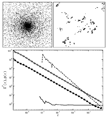
Figure 1: Top: left, $2d$ halo with $10000$ points and density given by eq. 1, with $\beta=1.5$; right, a fractal distribution with fractal dimension $D=1$ generated by a Levy-flight algorithm ($8000$ points). Bottom: Average conditional density for the set in the top left frame (empty circles) and the Levy flight fractal (filled circles). It is apparent that the two distributions have the same scaling in $\Gamma^{*}(r)$. The density profile of the halo with $\beta=1.5$ (dashed line) is steeper than the corresponding $\Gamma^{*}(r)$. The $\Gamma^{*}(r)$ for a halo with $\beta=0.5$ is shown by the solid line.

For $\beta>d/2$, instead, the second term dominates and the average conditional density is a power law with exponent $d-2\beta$ at any scale. This behavior appears therefore identical to the one of a fractal sample with dimension $D=2d-2\beta$. In fig. 1 we show that a halo and a fractal can have precisely the same scaling in $\Gamma^{*}(r)$, even though they are completely different systems.

In the light of this result, however, there has been little effort to clarify the difference between the two possibilities in the analysis of LSS data and in N-body computer simulations

In principle, a distinction between different sets of points with the same two point correlation properties could be obtained using box counting methods [28]. For the system described by eq. (1), we have:

$$\chi(q)=\lim_{l\rightarrow 0}\sum\mu_{i}^{q}=\lim_{l\rightarrow 0}(B_{1}(\beta,q)l^{q(d-\beta)}+B_{2}(\beta,q)l^{d(q-1)}),$$ (3)

where $l$ is the box size, $\mu_{i}$ is the mass inside the box $i$ and the sum extends over all the boxes; $B_{1}(\beta,q)$ and $B_{2}(\beta,q)$ are constants, depending on $\beta$ and $q$, but not on $l$ and $\chi(q)$ is the partition function. From eq. (1) it is easy to find the multifractal spectrum for the system: for $q<\frac{d}{\beta}$, $\alpha=d$ and $f(\alpha)=d$; for $q>\frac{d}{\beta}$ $\alpha=d-\beta$ and $f(\alpha)=0$. The exponent $\alpha$ describes the scaling of the mass inside a box of size $l$ as $l\rightarrow 0$, and $N\propto l^{-f(\alpha)}$ is the number of such boxes. Such results reveal a homogeneous ($f(\alpha)=d$) distribution of boxes whose average density $\rho(l)\propto l^{\alpha}/l^{d}=l^{d}/l^{d}$ is constant and a finite ($f(\alpha)=0$) set of boxes (in this case only one), whose average density scales as $\rho(l)\propto l^{\beta-d}$.

The multifractal analysis, therefore, correctly detects the presence of the central singularity and of an analytic distribution everywhere else. However, if we consider a system described by eq. (1), but made of discrete set of points, the identification of scalings by box counting analysis is no more straightforward. Since the system is not uniform, the local interparticle distance $\lambda$ is a function of the distance from the center $r$: $\lambda(r)=\left(A^{-1}r^{\beta}\right)^{1/d}$. It is easy to see that, if one considers boxes of size $l>l_{o}=A^{-1/d}$ (where $A$ is the amplitude in eq. (1)), they are occupied on average. If, on the other hand, $l<l_{o}$, one can define a characteristic distance $r_{o}$ from the center by the equation $\lambda(r_{o})=l$. The boxes at distances $r>r_{o}$ contain on average one or no particles, while the boxes at $r<r_{o}$ are on average occupied. In other words, there is a $l$-dependent scale $r_{o}$ below which the system is analogous to the continuum case, and above which the system looks intrinsically discrete.

A major difference between a fractal (or a multifractal) and a halo described by eq. (1) is the fact that, in the fractal, the density fluctuations are large at any scale. In the halo, instead, the density varies smoothly. A valid candidate to quantify such fluctuations is the conditional variance, defined as the mean square density fluctuation in spheres centered on points of the system, normalised to the average conditional density (eq. (2)) [29]:

$$\sigma_{c}^{2}(r)=\frac{\langle\rho_{R}(r)^{2}\rangle_{c}-\langle\rho_{R}(r)\rangle^{2}_{c}}{\langle\rho_{R}(r)\rangle^{2}_{c}},$$ (4)

where $\rho_{R}(r)$ is the density in a sphere centered in $R$ with radius $r$, and the subscript $c$ means that the corresponding quantities are “conditional”. In particular, $\langle\rho_{R}(r)^{2}\rangle_{c}$, where the average $\langle...\rangle_{c}$ is performed over all occupied points, can actually be rewritten as $\langle\rho_{R}(r_{0})\rho_{R}(r)\rho_{R}(r)\rangle$ where the average $\langle...\rangle$ is performed over all the $\vec{r_{0}}$ in the volume. In turn, $\langle\rho_{R}(r_{0})\rho_{R}(r)\rho_{R}(r)\rangle$ is actually the three point correlation function $\langle\rho_{R}(r_{i})\rho_{R}(r_{j})\rho_{R}(r_{K})\rangle$ with $r_{i}=r_{j}$. This shows that $\langle\rho_{R}(r)^{2}\rangle_{c}$ is in fact closely related to the three-point correlation function

In general, for a point distribution, $\sigma_{c}^{2}(r)$ will be given by the sum of two terms: $\sigma_{c}^{2}(r)=\sigma^{2}_{P}(r)+\sigma^{2}_{i}(r)$, where $\sigma^{2}_{P}(r)=(\langle\rho_{R}(r)\rangle_{c}V(r))^{-1}$ is the variance due to Poissonian noise and $\sigma^{2}_{i}(r)$ is the intrinsic variance of the system, which depends on its specific properties.

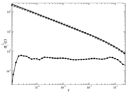
Figure 2: Normalized conditional variance $\sigma_{i}^{2}(r)$ for the samples described in fig. 1. Solid line with squares: fractal; empty circles: halo. Solid line: theoretical result from eq. (5)

It is possible to compute $\sigma^{2}_{i}(r)$ for a cluster described by eq. (1):

$$\sigma^{2}_{i}(r)=\frac{1}{d-\beta}\cdot\frac{\left[\frac{1}{d-3\beta}\left(1-r^{d-3\beta}\right)+\frac{d^{2}r^{d-3\beta}}{(d-\beta)^{3}}\right]}{\left\{\frac{1}{d-2\beta}+r^{d-2\beta}\left[\frac{d}{(d-\beta)^{2}}-\frac{1}{d-2\beta}\right]\right\}^{2}}-1.$$ (5)

From eq. (5) it is easy to see that for $\beta>d/2$, $\sigma^{2}_{i}(r)\propto r^{\beta-d}$. On the contrary, since a fractal is a scale invariant structure, $\sigma^{2}_{i}(r)$ (often referred to as lacunarity [29, 30, 31]) is constant. In fig. 2 we plot $\sigma^{2}_{i}(r)$ for a fractal and a halo, together with the analytic result of eq. (5).

In addition to the conditional variance we introduce a new statistical concept, the “scaling gradient” $\Delta$, which permits also a local analysis of the fluctuations.

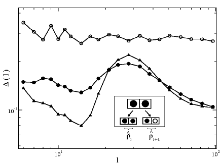
Figure 3: Measure of the scaling gradient $\Delta(l)$ as a function of the box size $l$ for different samples in $3d$. Empty circles: a fractal with dimension $D=2$ generated by a Levy flight algorithm. Filled circles: a halo with $\beta=2$. Triangles: a homogenous set. In the inset, the procedure followed to measure $\Delta(l)$ in $1d$: two adjacent occupied boxes (the boxes with filled circles) are divided in two offsprings each. The offsprings of the left box are both occupied ($\hat{\rho}=1$); while just one of the offsprings of the right one is occupied ($\hat{\rho}=1/2$). The resulting $\Delta$ is $1/2$.

Consider a point distribution in $d$ dimensions extending over a finite volume. The volume is divided in $N_{box}$ identical boxes of size $l$, with the number of occupied boxes being $N_{occ}(l)$.

We identify all the adjacent pairs of occupied boxes $N_{i}(l)$, where $i$ runs over all the occupied adjacent boxes, $N_{adj\_occ}$. Each box i of the occupied ones is divided in $N_{s}(i)$ identical boxes (offsprings); some of these will be occupied and we denote them as $N_{s\_occ}(i)$. $N_{s\_occ}(i)$ is the number of occupied offsprings in the box i and let us define $\hat{\rho}_{i}=N_{s\_occ}(i)N_{s}(i)^{-1}$ as the fraction of occupied offsprings of the box $i$.

The scaling gradient of the system is defined as:

$$\Delta(l)=\frac{1}{N_{occ}(l)}\sum_{i=1}^{N_{adj\_occ}}|\hat{\rho}_{i}(l)-\hat{\rho}_{i+1}(l)|,$$ (6)

where the sum extends over all pairs of adjacent occupied boxes $N_{adj\_occ}$. This measure has the following properties:

(i) it is a conditional measure, since it only considers occupied adjacent pairs;

(ii) it considers the occupation density $\hat{\rho}$, which is a measure of how the occupation of the boxes scales in the system;

(iii) it is sensitive to local fluctuations of $\hat{\rho}$, although it is averaged over the whole system.

In other words, the scaling gradient measures the fluctuations of the fragmentation properties of the system.

The results of a measure of $\Delta(l)$ in three different $3d$ samples are shown in fig. 3. While the measure of $\Delta(l)$ for the homogeneous set and the halo shows a peak at a characteristic scale, the fractal distribution has a flat $\Delta(l)$.

The behavior of $\Delta(l)$ for the halo can be explained as follows. For $l$ such that $r_{o}(l)=(Al^{3})^{1/\beta}>>1$ all boxes and their “offsprings” are occupied: in this case, $\Delta(l)\simeq 0$. When $l$ is such that $r_{o}(l)$ $\stackrel{{\scriptstyle<}}{{\scriptstyle{\sim}}}$ $1$, all the boxes are occupied, but some of their “offsprings” (with distance from the center $r\simeq 1$) will be empty. Therefore $\Delta(l)$ grows. Eventually, when $l$ is such $r_{o}(l)\simeq 1$, all the boxes will be occupied on average. Consider now the generation of box offsprings in this case: their size is such that a large number of them is empty. In particular, it is the maximum number of empty boxes deriving from occupied boxes. For this reason, $\Delta(l)$ reaches a maximum. This is apparent in fig. 3. On the contrary, since a fractal is a scale invariant structure, $\Delta(l)$ is constant at all scales larger than the lower cut-off. The scaling gradient is therefore able to detect unambiguously the scaling properties of different systems characterised by the same two-point correlations.

In summary, N-body simulations provide evidence for the formation of halos, clusters which are not really fractals, but still are characterized by power law correlations. The galaxy distribution, instead, appears more compatible with the fractal behaviour in a range of scales. We have addressed the fundamental issue of the discrimination between the two distributions in such a way to offer a series of tools which permit clarification of this problem. This requires going beyond the two point correlations, although with a careful critical analysis. For example, we show that the multifractal approach is not suitable in this respect. The conditional variance is more appropriate for the global properties at large scales, but for the more relevant case of local scaling, we introduce the new concept of “scaling gradient”. These methods and their critical analysis will represent a crucial element for extracting the relevant statistical properties in future large galaxy catalogues and N-body simulations.

- [1] \NameG. de Vaucouleurs, \REVIEWScience 167 1970 1203.
- [2] \NameR. M. Soneira, P.J.E. Peebles \REVIEWAstrophys. J. 211 1977 1S.
- [3] \NameB.B. Mandelbrot \REVIEWC. R. Acad. Sci. A 280 1975 1551.
- [4] \NameP.H. Coleman, L. Pietronero, R.H. Sanders \REVIEWAstron. Astrophys. 200 1988 32.
- [5] \NameL. Pietronero \REVIEWPhys. A, 144 1987 257.
- [6] \NameP.J.E. Peebles \REVIEWPhys. D 38 1989 273.
- [7] \NameP.Coleman, L.Pietronero \REVIEWPhys. Rep. 213 1992 311.
- [8] \NameR. L. Carpenter \REVIEWBull. Am. Astron. Soc. 18 1986 971 .
- [9] \NameZ.G. Deng, Z. Wen, Y. Z. Liu \REVIEWIAUS 130 1988 555.
- [10] \NameV. J. Martinez et al. \REVIEWAstrophys. J. 357 1990 50.
- [11] \NameX. Luo, D. N. Schramm \REVIEWScience 256 1992 513.
- [12] \NameA. Provenzale, L. Guzzo, G. Murante \REVIEWMon. Not. R. Astron. Soc. 266 1994 524.
- [13] \NameL. Guzzo \REVIEWNew Astr. 2 1997 517.
- [14] \NameF. Sylos Labini, M. Montuori, L. Pietronero \REVIEWPhys. Rep. 293 1998 61.
- [15] \NameR. Scaramella et al. \REVIEWAstron. Astrophys. 334 1998 404.
- [16] \NameK.K.S. Wu, O. Lahav, M.J. Rees \REVIEWNature 397 1999 225.
- [17] \NameV. J. Martinez \REVIEWScience 284 1999 445.
- [18] \NameJ. Pan, P. Coles \REVIEWMon. Not. R. Astron. Soc. 330 2002 719.
- [19] \NameR. Valdarnini, S. Borgani, A. Provenzale \REVIEWAstrophys. J. 394 1992 422.
- [20] \NameP.J.E. Peebles \REVIEWAstron. Astrophys. 32 1974 197.
- [21] \NameB. Moore et al. \REVIEWAstrophys. J. 524L 1999 19.
- [22] \NameN. Bahcall \REVIEWAnn. Rev. Astron. Astrophys. 26 1988 631.
- [23] \NameI. Zehavi et al. \REVIEWastro-ph/03012802003.
- [24] \NameG. Murante et al. \REVIEWMon. Not. R. Astron. Soc. 291 1997 585.
- [25] \NameJ.McClelland, J.Silk \REVIEWAstrophys. J. 217 1977 331 .
- [26] \NameA. Cooray, R. Sheth \REVIEWPhys. Rep. 372 2002 1.
- [27] \NameJ. Navarro, C. Frenk, S. D. M. White \REVIEWAp.J. 462 563 1996 .
- [28] \NameJ. Feder \BookFractals \PublPlenum Press, New York \Year1988.
- [29] \NameY. Gefen, B. B. Mandelbrot, A. Aharony \REVIEWPhys. Rev Lett. 45 1980 855.
- [30] \NameB.B. Mandelbrot \REVIEWProgress in Probability 37 1995 15.
- [31] \NameR. Blumenfeld , R.C. Ball \REVIEWPhys. Rev E 47 1993 2298. \NameV. J. Martinez, E. Saar in SPIE Proceedings ”Astronomical Data Analysis II \EditorJ.-L. Stark, F. Murtagh 4847, \Page86\Year2002.