Distributions of the Baryon Fraction on Large Scales in the Universe

Abstract

The nonlinear evolution of a system consisting of collisional baryons and collisionless dark matter is generally characterized by strong shocks and discontinuities in the baryon fluid. The baryons slow down significantly at postshock areas of gravitational strong shocks, which can occur in high overdense as well as low overdense regions. On the other hand, the shocks do not affect the collapse of the dark matter. Consequently, the baryon fraction would be nonuniform on large scales. We studied these phenomena with simulation samples produced by the weighted essentially nonoscillatory (WENO) hybrid cosmological hydrodynamic/$N$-body code, which is effective at capturing shocks and complex structures with high precision. We find that the baryon fraction in high mass density regions is lower on average than the cosmic baryon fraction, and many baryons accumulate in the regions with moderate mass density to form a high baryon fraction phase (HBFP). In dense regions with $\rho/\bar{\rho}>100$, which are the possible hosts for galaxy clusters, the baryon fraction can be lower than the cosmic baryon fraction by about 10%–20% at $z\simeq 0$. We also find that at $z<2$, almost all the HBFP gas locates in the regions with mass density $0.5<\rho/\bar{\rho}<5$ and temperature $T>10^{5}$ K, and conversely, almost all the gas in the areas of $0.5<\rho/\bar{\rho}<5$ and with temperature $T>10^{5}$ K has high baryon fraction. Our simulation samples show that about 3% of the cosmic baryon budget was hidden in the HBFP at redshift $z=3$, while this percentage increases to about 14% at the present day. The gas in the HBFP cannot be detected either by Ly$\alpha$ forests of QSO absorption spectra or by soft X-ray background. That is, the HBFP would be missed in the baryon budget given by current observations.

1 Introduction

Although the universe is dominated by dark matter and dark energy, the observed luminous universe exists in the form of baryonic matter. The primordial nucleosynthesis predicts $0.015<\Omega_{b}h^{2}<0.021$ (Walker et al. 1991; Esposito et al. 2000) The best fitting of cosmological parameters with the temperature fluctuations of the cosmic microwave background (CMB) radiation and large-scale structure clustering shows that the mass density of baryonic mater is $\Omega_{b}=0.0224\pm 0.0009$ $h^{-2}$ and the total matter density $\Omega_{m}=0.135^{+0.008}_{-0.009}$ $h^{-2}$ (Bennett et al. 2003). Therefore, the cosmic baryon fraction is $f_{c}\equiv\Omega_{b}/\Omega_{m}=0.166^{+0.012}_{-0.013}$.

In the linear evolution of gravitational clustering perturbations, the density and velocity distributions of the baryonic gas (or intergalactic medium [IGM]) are the same as those of the dark matter field point-by-point on scales larger than the Jeans length. Even if the IGM is initially distributed differently from the dark matter, a linear growth mode will lead to the same distribution of the IGM as of dark matter (Bi et al. 1992; Fang et al. 1993; Nusser 2000; Nusser & Haehnelt 1999). Thus, in the linear regime, although the density distributions of both IGM and dark matter are inhomogeneous, the baryon fraction is uniform on scales larger than the Jeans length. However, observations show that the distribution of the baryon fraction probably is not uniform. X-ray measurements have revealed that the baryon fraction in galaxy clusters is less than the prediction of primordial nucleosynthesis (Ettori & Fabian 1999). This discrepancy is more serious in the cores of clusters (Sand et al. 2003). Even considering a depletion of baryons at the virial radius, the baryon fraction in galaxy clusters is still less than the predicted value (Ettori 2003). This indicates that in the nonlinear evolved fields, the baryon fraction distribution $f_{b}({\bf x})$ is spatially dependent, not equal to $f_{c}$ everywhere.

In this paper, we explore the formation and evolution for the nonuniform distribution of baryon fraction. On large scales, the nonuniformity of the baryon fraction is a result of the statistical discrepancy of baryonic gas from the underlying dark matter during nonlinear evolution. Recently, the statistical decoupling between baryonic gas and dark matter fields has been studied, both theoretically and numerically (Feng et al. 2003; He et al. 2004; Pando et al. 2004). These studies found that, although in both the linear and the nonlinear regimes the evolution of the IGM is dynamically governed by the gravity of the underlying dark matter field, the effects of the gravity in different regimes are very different. In the former, the gravity of the dark matter ensures that baryonic gas follows dark matter point-by-point, while in the latter, the gravity of the dark matter will inevitably lead to the decoupling of the baryonic gas from the dark matter on scales larger than the Jeans length. That is to say, the linear dynamical behavior of the baryonic matter can be simply obtained from the dark matter field via a similarity mapping (e.g., Kaiser 1986), while in the nonlinear regime, the similarity is broken. Obviously, a direct consequence of the baryon – dark matter discrepancy is the inhomogeneity of the baryon fraction distribution. We follow this clue to study the properties of the deviation of $f_{b}({\bf x})$ from $f_{c}$.

The outline of this paper is as follows. In §2 we describe the dynamical mechanism leading to the deviation of the baryon fraction from the cosmic value, together with the predictions from this mechanism. In §3 we present the samples used to numerically study the baryon fraction. In §4 we investigate the statistical features of the field $f_{b}({\bf x})$, and compare them with the predictions. Finally, conclusions and discussions are given in §5.

2 The mechanism leading to non-uniform distribution of baryon fraction

A dynamical mechanism of separating baryonic gas from dark matter was addressed in the early study of structure formation (Shandarin & Zel’dovich 1989). Because the dark matter particles are collisionless, the velocities of the dark matter particles are multivalued at the intersection of the dark matter particle trajectories. On the other hand, the IGM, as an ideal fluid, has a single-value velocity field. Thus, discontinuities, such as shocks or complex structures, will develop in the density and velocity fields of gas at the intersection of the dark matter particle trajectories. This leads to the decoupling between the mass and velocity fields of the IGM and the dark matter. This feature can also be seen with the self-similar solution of spherical collapse under the self-gravity of baryonic gas and dark matter given by Bertschinger (1985). It shows that an outgoing shock is always formed during the infall of baryons.

A shock is actually a common feature of IGM fluid. Although the cosmic baryonic gas is a Navier-Stokes fluid, the dynamic behavior of the IGM is dominated by the gravity of the growth modes of the dark matter. It has been recognized that the growth mode dynamics of cosmic baryonic gas can be approximately described by the random-force–driven Burgers equation (Gurbatov et al. 1989; Vergassola et al. 1994; Berera & Fang 1994; Jones 1999; Matarrese & Mohayaee 2002; Pando et al. 2004; He et al. 2004). The dynamical behavior of a Burgers fluid depends on two characteristic scales: (1) the correlation length of the random force (in our case, the gravity of dark matter), and (2) the Jeans length. When the former is larger than the latter, Burgers turbulence develops in the baryonic gas in the non-linear regime. That is, for the cosmic initial perturbations, which contain fluctuations on small as well as larger scales, the Burgers turbulence will definitely develop in nonlinear regime. The Burgers turbulence is qualitatively different from Navier-Stokes’ turbulence. The latter generally consists of vortices on various scales, while the former is a collection of shocks (Polyakov 1995; Bouchaud et al. 1995; Yakhot 1998; Lässig 2000; Davoudi et al. 2001). These features arise because the velocity field is irrotational. Thus, the IGM velocity field in the nonlinear regime can be understood as a field consisting of shocks.

Gas should slow down after passing through shocks, and postshock gas should have higher density. On the other hand, dark matter is not affected by the shocks. The nonuniform distribution of baryon fraction is then caused by the postshock slowdown of gas. Consequently, $F_{b}$ will be larger than 1 in the regions of postshock, which can be in high-density ($\rho/\bar{\rho}>5$) and low-density ($\rho/\bar{\rho}\simeq$ 1 - 5) regions.

Since the initial density perturbations of dark matter contain components that have correlation scales larger than the Jeans length at low density regions, the Burgers turbulence and the shocks can happen in low as well as high overdense regions. This property has also been shown in simulation results of He et al. (2004), who found that the shock heating is significant in the density regions of $\rho/\bar{\rho}\simeq 1-5$ at redshift $z\simeq 0$. Therefore, the postshock slowdown mechanism will take place in both high and low overdense regions.

Considering gas is moving from low- to high-density regions, the postshock slowdown mechanism leads to the distributions of $f_{b}({\bf x})$ having the following features.

1. Since all massive halos, at whatever redshift, formed by gravitational collapse, the baryon shortage in high overdense regions should be common at low as well as high redshifts.

2. Since baryons are detained on the way from low-density to high-density (collapsed) regions, the $f_{b}({\bf x})>f_{c}$ regions should be located in the low or moderate overdense areas surrounding high overdense area, like massive halos.

3. Since baryons are detained in the postshock regions, the $f_{b}({\bf x})>f_{c}$ regions tend to be located in the higher temperature regions.

4. Since baryons are frequently hampered by shocks, the velocities of baryonic gas are statistically lower than those of dark matter.

The last point has been analyzed in Pando et al. (2004), who showed that the probability distribution of baryons with large peculiar velocities is much less than that of dark matter.

3 Simulation samples

The hydrodynamic equations of the baryonic gas in the universe is the typical Navier-Stokes equation (Feng et al. 2004). As discussed in the last section, the baryonic gas in the nonlinear regime is characterized by (1) regions with discontinuities and strong shocks and (2) regions with smooth and simple variations of the field between the discontinuities. Therefore, an optimal simulation scheme should be effective at capturing shock and discontinuity transitions and in the meantime, at calculating piecewise smooth functions with a high resolution.

For these reasons we do not use numerical schemes based on smoothed particle hydrodynamic (SPH) algorithms. It is well known that one of the main challenges to the SPH scheme is how to handle shocks or discontinuities, because the nature of SPH is to smooth the fields considered (e.g., Børve et al. 2001; Omang et al. 2003). Instead, we apply an Eulerian approach to simulate the IGM. Among the popular algorithms of high-resolution shock capturing are the total variation diminishing (TVD) scheme (Harten 1983) and the piecewise parabolic method (PPM; Collella & Woodward 1984). Both schemes start from the integral form of conservation laws of Euler equations and compute the flux vector based on cell averages (finite volume scheme). These methods are able to produce relatively sharp, nonoscillatory shock transitions. However, the TVD scheme generally degenerates to first-order accuracy at locations of smooth extrema (Godlewski & Raviart 1996), and this problem is serious in calculating the difference between hydrodynamic quantities on both sides of the shock when the Mach number of a gas is high. This is exactly the case that is encountered in the gravitationally coupled IGM and dark matter system.

Later, the essentially nonoscillatory (ENO) and then the weighted essentially nonoscillatory (WENO) schemes were proposed as an improvement over the TVD and PPM schemes (Harten et al. 1986; Shu 1998; Fedkiw et al. 2003; Shu 2003). It has been shown that for solving problems governed by the high Reynolds number Navier-Stokes equations, the WENO is more efficient than the TVD and PPM schemes (Shi et al. 2003; Zhang et al. 2003). The WENO has been successfully applied to problems of astrophysical hydrodynamics, including stellar atmospheres (Del Zanna et al. 1998), high Reynolds number compressible flows with supernovae (Zhang et al. 2003), and high Mach number astrophysical jets (Carrillo et al. 2003). In the context of cosmological applications, the WENO scheme has proved especially adept at handling the Burgers equation (Shu 1999). Hence, we believe that the WENO scheme would be effective at studying the problems sensitive to strong shocks during the cosmological gravitational clustering.

Recently, a hybrid hydrodynamic/$N$-body code based on the WENO scheme was developed and has passed typical reliability tests, such as the Sedov blast wave and the formation of Zel’dovich pancakes (Feng et al. 2004). The code has been tested with capturing gravitational shocks during the large-scale structure formation (He et al. 2004). The WENO algorithm on cosmological problems can be found in Feng et al. (2004).

For the purpose of this paper, we use the same simulation samples as in He et al. (2004). The simulations were performed in a periodic, cubic box of size 25 $h^{-1}$Mpc with a 192³ grid and an equal number of dark matter particles. We use the clouds-in-cell method for mass assignment and interpolation and adopt the seven-point finite difference to approximate the Laplacian operator. The simulations start at redshift $z=49$, and the results are output at redshifts $z$=6, 4, 3, 2, 1, 0.5, and 0. The atomic processes, including ionization, radiative cooling, and heating, are modeled similarly as in Cen (1992) in a plasma of hydrogen and helium of primordial composition ($X=0.76$, $Y=0.24$). Processes such as star formation and feedback due to SNe and AGN activities are not taken into account yet. A uniform UV background of ionizing photons is assumed to have a power-law spectrum of the form $J(\nu)=J_{21}\times 10^{-21}(\nu/\nu_{HI})^{-\alpha}$ergs s^-1cm^-2sr^-1Hz^-1, with parameters $J_{21}=1.0$ and $\alpha=1$. The photoionizing flux is suddenly switched on at $z>10$ to heat the gas and reionize the universe.

For statistical studies, we randomly sampled 500 one-dimensional fields from the simulation results at each redshift. Each one-dimensional sample, of size $L$=25 $h^{-1}$ Mpc, contains 192 data points. For each of these points, information about the mass density and peculiar velocity of dark matter, as well as the mass density, peculiar velocity, and temperature of the IGM, is recorded. We emphasize that, since we mostly focus on one-point statistics, our results are dependent only on the fair sampling of these data points, which is not relevant to the sample dimensions.

4 Statistical properties of the baryon fraction

4.1 An example of the baryon fraction distribution

Figure 1 is an example of the one-dimensional spatial distribution of $F_{b}(x)$, which is the normalized baryon fraction $F_{b}(x)=f_{b}(x)/f_{c}$, and $x$ is the comoving coordinate. We also show in Figure 1 the mass densities $\rho_{DM}$ and $\rho_{IGM}$ of dark matter and baryonic matter and the temperature $T$ of the baryons. The mass densities $\rho_{DM}$ and $\rho_{IGM}$ are in units of their $\overline{\rho}_{DM}$ and $\overline{\rho}_{IGM}$, respectively. Figure 1 clearly shows that $F_{b}(x)$ is significantly nonuniform. Some small-scale deviation of $F_{b}(x)$ from unity can be explained by the Jeans smoothing. However, there are deviations on scales of one to a few $h^{-1}$ Mpc, which is larger than the corresponding Jeans length of the baryonic gas.

In Figure 1 the mass density on the left side of the simulation box is higher than on the right side, and from the comparison of density distributions at $z=0.5$ and $0$, one can see that matter is infalling from the right to the left region. We see a shock at about $x=11$ $h^{-1}$ Mpc at $z=0.5$. The temperature of preshock gas is $\sim$10³ K and increases to $\sim$10⁷K after passing through the shock. That is, the temperature increases by a factor of $\sim 10^{4}$. According to the shock theory of a polytropic gas with index $\gamma$ (Landau & Lifshitz 1959), the Mach number should be $M\simeq\sqrt{10^{4}}\simeq 100$. This value is reasonable, since under such a strong shock, the density of baryons is enhanced by a factor of $\sim(\gamma+1)/(\gamma-1)=4$, while the mass density of dark matter is not affected by the shock. Therefore, $F_{b}(x)$ can be as high as 4. The positions of this shock at time $z=0.5$ and $0$ indicate that it is an outgoing shock with respect to the high-density area. At $z=0.5$, the peak of $F_{b}(x)$ is just located on the postshock side or high-temperature side. At $z=0$, more high peaks of $F_{b}(x)$ develop behind the shock. Namely, more baryonic matter is detained by the shock. This result is consistent with the picture of postshock slow down of the baryon flow described in §2.

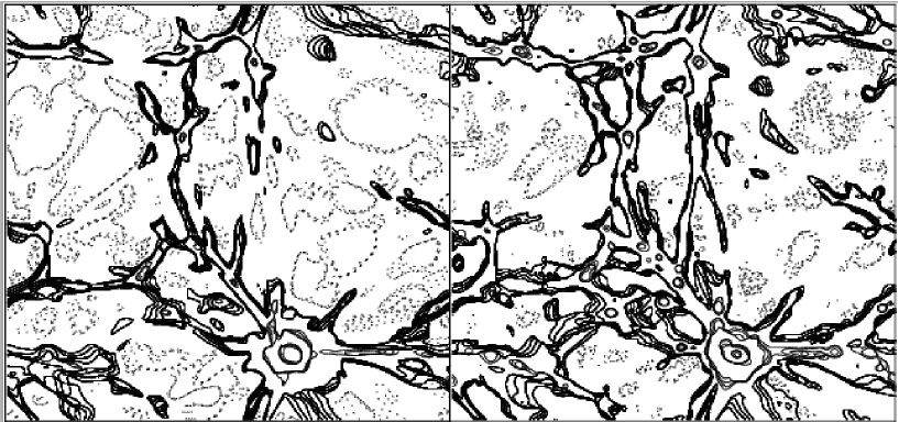
Figure 2: Density contour plots of dark matter (right panel) and baryonic gas (left panel) for a slice of 0.26 $h^{-1}$ Mpc thickness at $z=0$. The solid contours encompass the overdense regions with $\rho=e^{i/2}$, $i=0,1,2...$, ($\bar{\rho}$ is normalized to 1). The dotted lines represent the boundaries of the underdense regions with $\rho=e^{-i/2}$, $i=1,2...$.

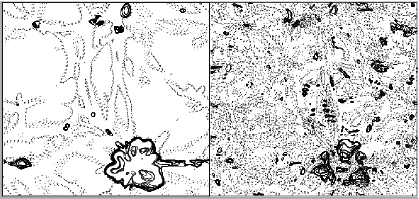
Figure 3: Contour plots of baryon-to-dark ratio $F_{b}$ (right panel) and temperature $T$ (left panel) for the same slice as in Fig. 2. The solid contours represent, respectively, the regions with $F_{b}=e^{i/3},i=0,1,2,...$ and $T=e^{i/2}\times 10^{5}$ K, $i=0,1,2,...$. The dotted lines represent $F_{b}=e^{-i/3},i=1,2,...$ and $T=e^{-i/2}\times 10^{5}$ K, $i=1,2,...$ regions.

This picture can be more clearly seen in Figures 2 and 3. Figure 2 presents two-dimensional contours of the baryonic gas and dark matter densities. One can see at the lower part of the plots that a massive halo on the scale of $\sim$5 $h^{-1}$ Mpc is formed. The $\rho_{IGM}>1$ region is obviously larger than the dark matter counterpart at $\rho_{DM}>1$. This means that more baryons remain in the low overdense area. This discrepancy cannot be caused by the Jeans diffusion. Figure 3 gives the two-dimensional contours of temperature and $\rho_{IGM}/\rho_{DM}$ (i.e., $F_{b}$) of the same slice in Figure 2. Figure 3 shows that the size of the high-temperature region is about the same as that of the $\rho_{IGM}>1$ region. From the right panel of Figure 3, we see that the contours of $F_{b}>1$ are located outside the center of the object. Conversely, the central part of this object, where the mass density is higher than that at the boundary, has only $F_{b}<1$. This feature is very common. All the clustered structures like the one in Figures 2 and 3 have $F_{b}<1$ in their center and are surrounded by $F_{b}>1$ regions. That is, baryons accumulate in low and moderate (dark matter) overdense areas.

4.2 Baryon fraction - density and baryon fraction - temperature relations

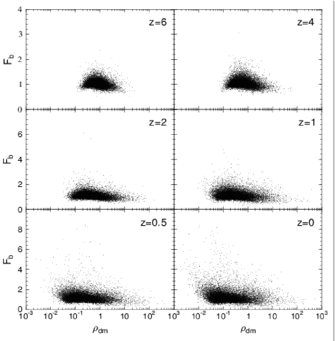
Figure 4: Relation between $F_{b}(x)$ and $\rho_{DM}(x)$ for each point $x$ at redshifts $z$=6, 4, 2, 1, 0.5, and 0. In each panel, the data consist of 19,200 points randomly drawn from the simulation samples. The density $\rho_{DM}$ is in units of ${\bar{\rho}}_{DM}$.

In Figure 4, we show the scatter plots between the baryon fraction and the dark matter density at redshifts $z$=6, 4, 2, 1, 0.5, and 0. Each panel in Figure 4 contains 19,200 data points of the randomly drawn 500 one-dimensional samples at each redshift. It is expected that, in each panel, most of the data points are distributed around $F_{b}\simeq 1$. If baryons underwent only linear evolution, all the points should be on the line of $F_{b}\simeq 1$ for all $\rho_{DM}$. However, the scatters around $F_{b}=1$ are significant, among which the relatively small scatters can be explained by the Jeans smoothing, while the points with $F_{b}\gg 1$ should be attributed to strong shocks or discontinuity transitions. These points are especially prominent in the regions of $\rho_{DM}<5$.

We can see from Figure 4 that the scatter of $F_{b}$ at redshifts $z\simeq 2$ is as significant as that at low redshifts. Only at $z\geq 4$ does the $F_{b}$ scatter become small. This is consistent with the prediction in §2 that the deviation of $F_{b}$ from 1 at early times should be as prominent as that at later times. This feature is much different from the virialization of baryons in collapsed massive halos. The virialization process generally takes place during the formation of the halos, while the shortage of baryons in massive halos proceeds prior to the formation of the halos.

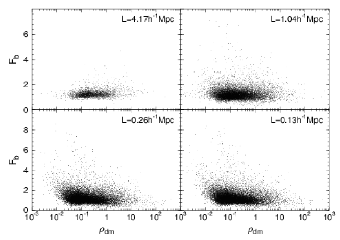
Figure 5: Relation between $F_{b}$ and $\rho_{DM}$ for data smoothed on scales 0.13, 0.26, 1.04, and 4.17 $h^{-1}$ Mpc at $z=0$.

Figure 5 gives the relation between the baryon fraction and the dark matter density at $z=0$ for baryon and dark matter fields smoothed on scales 0.26, 1.04, and 4.17 $h^{-1}$ Mpc, respectively (the method of smoothing is given in Appendix A). By this treatment, the linear size of each cell will increase by factors of $2$, $2^{3}$, and $2^{5}$, respectively. We see that the scatter of the smoothed $F_{b}$ on the scale 1.04 $h^{-1}$ Mpc remains nearly the same as that on the scale 0.13 $h^{-1}$ Mpc even when $\rho_{DM}<1$. Since the size of high-$F_{b}$ regions is generally larger than 1 $h^{-1}$ Mpc (see Figs 1, 2, and 3), the scatter cannot be erased by smoothing on scales of about 1 $h^{-1}$ Mpc. Therefore, the scatter is intrinsic.

As a quantitative comparison for the dependence of $F_{b}$ on the dark matter density, in Table 1 we list the mean baryon fraction in each density interval at several redshifts. We see from Table 1 that at all redshifts from 0 to 4, the mean $F_{b}$ is always in the range of 0.7 to 0.9 for the very high densities. Since such high-density areas are the possible sites for the formation of galaxy clusters, this result provides a cosmological explanation of the shortage of baryons in dense dark halos, like galaxy clusters. We can see that the baryon fraction of clusters can be as low as $\sim 0.8$ in general.

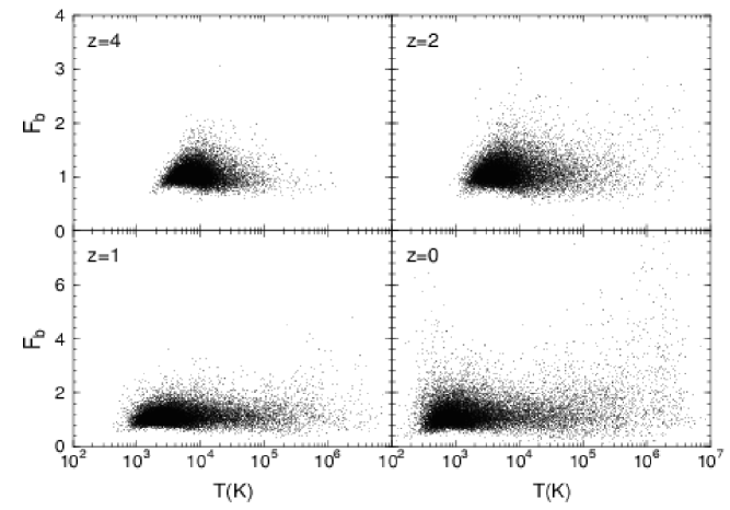
Figure 6: Relation between $F_{b}(x)$ and temperature $T(x)$ for each point $x$ at redshifts $z$=4, 2, 1, and 0. The data consist of 19,200 points randomly drawn from the simulation samples.

In Figure 6, we show the relations between baryon fraction and temperature of baryonic gas at redshifts $z$=4, 2, 1, and 0. Each panel in Figure 6 contains 19,200 data points of the randomly drawn 500 samples at each redshift. The $z$-evolution of $F_{b}$ in $T$-space is different from that of $\rho_{DM}$-space. In Figure 4 the high-$F_{b}$ points are always in the density range $0.5<\rho_{DM}<5$ for all redshifts considered, while in Figure 6, the high-$F_{b}$ points are mostly located at $10^{4}<T<10^{5}K$ for $z=4$ and $T>10^{5}$ K for $z=0$. That is, the baryonic gas with $F_{b}>1$ generally tends to lie in high-temperature ($T>10^{5}$ K) areas. This is consistent with the picture that strong shocks can reduce the flow of the baryons in postshock areas and meanwhile increase the gas temperature by a factor of $10^{2}$-$10^{4}$ (Fig. 1).

4.3 High baryon fraction phase (HBFP)

From Figures 4 and 6, we see that almost all the baryonic gas with $F_{b}>1$ is hot ($T>10^{5}$ K) and moderately dense ($\rho_{DM}<5$). From these results, we can define a special phase of baryonic gas with the indicator $F_{b}>1$: it can be called high baryon fraction phase (HBFP). Baryonic gas in the HBFP is characterized by two properties: (1) it is located mostly in the moderately dense regions with $\rho_{DM}<5$, and (2) its temperature is larger than $10^{5}$ K (see §4.2). Conversely, Figure 7 indicates that almost all the gas with $\rho_{DM}<5$ and $T>10^{5}$ K has mean $F_{b}$ larger than 1. Figure 8 is another version of Figure 7, which shows the $\rho_{DM}$-dependence of the mean baryon fraction for baryonic gas with $T<10^{5}$ K and $T>10^{5}$ K. It also indicates that almost all the gas with $T>10^{5}$ K and $\rho_{DM}<5$ are $F_{b}>1$. More precisely, 89% baryons in the $T>10^{5}$ K and $\rho_{DM}<5$ regions are $F_{b}>1$. Thus, the phase of $F_{b}>1$ is approximately equivalent to the thermodynamic condition $T>10^{5}$ K and $\rho_{DM}<5$. The HBFP is a special phase of baryonic gas formed as a result of the nonlinear evolution of baryon–dark matter systems.

Figure 9 is the same as the $z=0$ panel of Figure 8, but with data smoothed on scales 0.26, 1.04, and 4.17 $h^{-1}$ Mpc. All the basic features of Figure 9 are the same as those of Figure 8. That is, $\overline{F_{b}}<1$ is generally in regions with high density and high temperature, while $\overline{F_{b}}>1$ is mostly in $T>10^{5}$ K, but with lower $\rho_{DM}$. In the range $0.03<\rho_{DM}<1$, the curves of $F_{b}$ in Figure 9 are clearly less sensitive to smoothing scales. This shows that shot noise does not affect our conclusions about the mean baryon fractions (see Appendix B).

On large enough scales, the cosmic clustering can still remain in the linear regime, and therefore one may expect that the inhomogeneity of baryon fraction distribution would disappear on large scales. The mean baryon fraction within a large radial region around a cluster has to be asymptotically approaching 1. Figure 9 shows that $\overline{F_{b}}$ is still quite inhomogeneous even at a scale as large as 4.17 $h^{-1}$ Mpc. Therefore, the asymptotic radius for $F_{b}\rightarrow 1$ should be larger than 4 $h^{-1}$ Mpc.

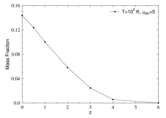
Figure 10: The $z$-evolution for the mass fraction of the HBFP (high baryon fraction phase) in the total baryonic matter.

In terms of observations, the HBFP is very different from other phases of the baryonic gas. As for the mass density, the HBFP is about the same as the IGM for Ly$\alpha$ forests, which is given by the absorption of HI in the regions $0.5<\rho_{DM}<5$ (Bi & Davidsen 1997). However, the HBFP cannot be detected by the Ly$\alpha$ forests of QSO’s absorption spectrum, because the fraction of $HI$ is too low to be seen when temperature $T$ is higher than $10^{5}$ K. As for the temperature, the HBFP is about the same as the so-called WHIM (warm hot IGM) (Cen & Ostriker 1999), which is generally defined as baryonic gas with temperature $10^{5}-10^{7}$ K, located in the regions close to the filaments, with mass density $5<\rho_{DM}<200$ (Davé et al. 2001). The WHIM would be a source of soft X-ray background. However, the number density of the HBFP gas is too low for it to be a source of soft X-ray emissions, and hence it cannot be detected via the soft X-ray observations either. For these reasons, the HBFP baryons are out of the baryon budget counted with the current observations. The contribution of the HBFP to the total cosmic baryon budget is given in Figure 10. The mass fraction of HBFP in the baryon budget is about 2.5% at $z=$ 3 and increases to 14.4% at the present day ($z=0$). Therefore, the HBFP would not be a negligible component of the missing baryons.

5 Conclusions and Discussions

In the nonlinear regime, a system consisting of collisional baryons and collisionless dark matter is generally characterized by strong shocks and discontinuities in the baryonic fluid. The shocks outgoing from high-density regions generally slow down the infall motion of baryons from low-density to high-density regions. Consequently, the baryon fraction in lower overdense areas is higher than the cosmic value, while in higher overdense areas it is lower than the cosmic value. We use $N$-body/hydrodynamic simulation samples produced by the WENO code to quantitate the deviation of the baryon fraction from cosmic value. We conclude that the overall baryon matter of massive halos like clusters is lacking by about 10%–20%. We also find that the HBFP is composed of the gas with $T>10^{5}$K and is located in moderate-density ($\rho_{DM}<5$) regions.

Thus, in terms of the baryon fraction, gas in massive halos, like clusters, is in the phase of low baryon fraction, while gas with $\rho_{DM}<5$ and $T>10^{5}$K is in HBFP. Both the low baryon fraction phase and HBFP are formed by the same mechanism of the shock-caused separation between the baryonic gas and dark matter. About 14% baryons in the universe today are presumably hidden in the HBFP. The HBFP can be traced neither by QSO absorption spectrum nor by X-ray emissions. However, the ionized electrons in the HBFP would be capable of scattering CMB photons and might generate secondary cosmic temperature fluctuations. The Sunyaev-Zel’dovich effects might be promising for detecting the existence of the HBFP.

We should point out that star formation and their feedback on the IGM evolution are not considered in our simulation. Generally speaking, there are two types of feedbacks: (1) photoionization heating by the UV emission of stars and AGNs and (2) injection of hot gas and energy by supernova explosions or other sources of cosmic rays. The photoionization heating actually can be properly considered, if the UV background is adjusted by fitting the simulation with the observed mean flux decrement of QSO Ly$\alpha$ absorption spectra (Feng et al. 2003). The effect of injecting hot gas and energy by supernovae is localized in massive halos, and thus it may change some results with clusters but does not affect the IGM in low- and moderate-density areas. Therefore, the features of the HBFP would not be significantly affected even if considering the effect of star formation.

Appendix A Smoothing with scaling functions

Consider a one-dimensional density fluctuation $\delta(x)$ on a spatial range from $x=0$ to $L$. We divide the space into $2^{j}$ segments labeled $l=0,1,...2^{j}-1$, each of size $L/2^{j}$. The index $j$ is a positive integer and gives length scale $L/2^{j}$. The larger the value of $j$, the smaller the length scale. The index $l$ represents the position and corresponds to the spatial range $lL/2^{j}<x<(l+1)L/2^{j}$. Hence, the space $L$ is decomposed into cells $(j,l)$.

The discrete wavelet is constructed such that each cell $(j,l)$ supports a compact function, the scaling function $\phi_{j,l}(x)$. In our calculations, the Daubechies 4 (D4) wavelet (Daubechies 1992) is used. The scaling function satisfies the orthogonal relation

$$\int\phi_{j,l}(x)\phi_{j,l^{\prime}}(x)dx=\delta^{K}_{l,l^{\prime}},$$ (A1)

where $\delta^{K}$ is Kronecker delta function. The scaling function $\phi_{j,l}(x)$ is a window function on scale $j$ centered at the segment $l$. The normalization of the scaling function is $\int\phi_{j,l}(x)dx=(L/2^{j})^{1/2}$.

For a field $\rho(x)$, its mean in cell $(j,l)$ can be estimated by

$$\rho_{j,l}=\frac{\int_{0}^{L}\rho(x)\phi_{j,l}(x)dx}{\int_{0}^{L}\phi_{j,l}(x)dx}=\left(\frac{2^{j}}{L}\right)^{1/2}\epsilon^{\rho}_{j,l},$$ (A2)

where $\epsilon^{\rho}_{j,l}$ is called the scaling function coefficient (SFC), given by

$$\epsilon^{\rho}_{j,l}=\int_{0}^{L}\rho(x)\phi_{j,l}(x)dx.$$ (A3)

A one-dimensional field $\rho(x)$ can be decomposed into

$$\rho(x)=\sum_{l=0}^{2^{j}-1}\epsilon^{\rho}_{j,l}\phi_{j,l}(x)+O(\geq j).$$ (A4)

The term $O(\geq j)$ in equation (A4) contains only the fluctuations of the field $F(x)$ on scales equal to and less than $L/2^{j}$. This term does not have any contribution to the window sampling on scale $j$. Thus, for a given $j$, the one-point variables $\rho_{j,l}$ or $\epsilon^{\rho}_{j,l}$ ($l=0,1...2^{j}-1$) give a complete description of the field $F(x)$ smoothed on scale $L/2^{j}$. As one-point variables the $\epsilon^{\rho}_{j,l}$ are similar to the measure given by count-in-cell technique. However, the orthonormality equation (A1) ensures that the set of $\rho_{j,l}$ or $\epsilon^{\rho}_{j,l}$ does not cause false correlations. When the “fair sample hypothesis” (Peebles 1980) holds, the average over the ensemble of the random field can be estimated by averaging over modes $(j,l)$.

Appendix B Errors of Poisson sampling

Consider a random field $\rho^{M}(x)=\bar{\rho}[1+\delta(x)]$, where $\delta(x)=[\rho(x)-\bar{\rho}]/\bar{\rho}$, and $\bar{\rho}$ is the mean. Obviously, $\langle\delta(x)\rangle=0$. The observed or simulated field $\rho(x)$ is considered to be a Poisson sampling of the field $\rho^{M}(x)$. The characteristic function of the $\rho(x)$ is

$$Z[e^{i\int\rho(x)u(x)dx}]=\exp\left\{\int dx\rho^{M}(x)[e^{iu(x)}-1]\right\},$$ (B1)

and the statistic of $\rho(x)$ is given by

$$\langle\rho(x_{1})...\rho(x_{n})\rangle_{P}=\frac{1}{i^{n}}\left[\frac{\delta^{n}Z}{\delta u(x_{1})...\delta u(x_{n})}\right]_{u=0},$$ (B2)

where $\langle...\rangle_{P}$ is the average for the Poisson sampling. We then have

$$\langle\rho(x)\rangle_{P}=\rho^{M}(x),$$ (B3)

and

$$\langle\rho(x)\rho(x^{\prime})\rangle_{P}=\rho^{M}(x)\rho^{M}(x^{\prime})+\delta^{D}(x-x^{\prime})\rho^{M}(x).$$ (B4)

Subjecting equations (B3) and (B4) to the transform equation (A2), we have

$$\langle\rho_{j,l}\rangle_{P}=\rho^{M}_{j,l}$$ (B5)

and

$$\langle\rho_{j,l}\rho_{j,l}\rangle_{P}=\rho^{M}_{j,l}\rho^{M}_{j,l}+\frac{2^{j}}{L}\int\rho^{M}(x)\phi_{j,l}(x)\phi_{j,l}(x)dx.$$ (B6)

Therefore, the Poisson sampling error of the measurement $\rho_{j,l}$ can be estimated by

$$\sigma^{2}_{j,l}\equiv\langle\rho_{j,l}\rho_{j,l}\rangle_{P}-\langle\rho_{j,l}\rangle^{2}_{P}=\frac{2^{j}}{L}\int\rho^{M}(x)\phi_{j,l}(x)\phi_{j,l}(x)dx.$$ (B7)

If we use the normalized density variable, equation (B7) gives

$$\sigma^{2}_{j,l}=\left\langle\frac{\rho_{j,l}}{\bar{\rho}}\ \frac{\rho_{j,l}}{\bar{\rho}}\right\rangle_{P}-\left\langle\frac{\rho_{j,l}}{\bar{\rho}}\right\rangle^{2}_{P}=\frac{2^{j}}{L}\frac{1}{\bar{\rho}}+\frac{2^{j}}{L}\int\frac{\delta(x)}{\bar{\rho}}\phi_{j,l}(x)\phi_{j,l}(x)dx.$$ (B8)

Since the Poisson samplings for different modes $(j,l)$ are uncorrelated, the Poisson sampling error of the measurement of $(1/N)\sum_{N}\rho_{j,l}$, which is the mean of $\rho_{j,l}$ over $N$ modes, is

$$\frac{1}{N}(\sum_{N}\sigma^{2}_{j,l})^{1/2}=\frac{1}{N}\left[N\frac{2^{j}}{L}\frac{1}{\bar{\rho}}+\sum_{N}\frac{2^{j}}{L}\int\frac{\delta(x)}{\bar{\rho}}\phi_{j,l}(x)\phi_{j,l}(x)dx\right]^{1/2}.$$ (B9)

Considering that $\langle\delta(x)\rangle=0$, the second term on the right-hand side generally is negligible, and we then have

$$\frac{1}{N}(\sum_{N}\sigma^{2}_{j,l})^{1/2}\simeq\frac{1}{\sqrt{N}}\left(\frac{1}{(L/2^{j})\bar{\rho}}\right)^{1/2},$$ (B10)

where $N$ is the number of modes. The factor $(L/2^{j})\bar{\rho}$ is the mean mass, or mean number of particles in the cell $L/2^{j}$. A smoothed field takes a larger $(L/2^{j})$. Thus, if a statistical result is weakly dependent on the $(L/2^{j})$-smoothing, the effect of Poisson error is negligible.

In some calculations, we only choose the modes for which the density is restricted to a given range. The average over these modes may not give $\langle\delta(x)\rangle=0$. In this case, the $\delta(x)$ term in equation (B8) is not negligible. For instance, if $\langle\delta(x)\rangle\simeq 100$, the error would be increased by a factor of 10. Nevertheless, the contribution of the $\delta(x)$ term is also proportional to $2^{j}/L$. If a statistical average over $500$ modes with mean number density is larger than $0.03$, the Poisson error will not be larger than 25%. Therefore, in Figures 7–9, the shot noise in the range of $\rho_{DM}>0.03$ are negligible.

Figure 1: Example of the one-dimensional distribution of $F_{b}(x)$ at $z$=0 and 0.5, where $x$ is the comoving coordinate. The corresponding temperature and density fields are also shown in the bottom panels.

Figure 7: Averaged $F_{b}$ vs. temperature $T$. The three curves are for (1) the total samples (solid lines), (2) the data with $\rho_{DM}<5$ (dotted lines), and (3) the data with $\rho_{DM}>5$ (dashed lines).

Figure 8: Averaged $F_{b}$ vs. $\rho_{DM}$. The three curves are for (1) the total samples (solid lines), (2) the data with temperature $T<10^{5}$ K (dashed lines), and (3) the data with $T>10^{5}$ K (dotted lines).

Figure 9: Same as Fig. 8, but only for $z=0$, and the data are smoothed on scales of 0.26, 1.04, and 4.17 $h^{-1}$ Mpc, respectively.

Table 1: Mean $F_{b}$ for Mass Density $\rho_{DM}$ and Redshift $z$

$\rho_{DM}$ ($\bar{\rho}_{DM}$)	$z$=0	z=0.5	z=1	z=2	z=3	z=4
0.03 – 0.5	1.23	1.20	1.17	1.12	1.09	1.06
0.5 – 5.0	1.17	1.11	1.07	1.05	1.04	1.03
5.0 – 100	1.11	1.00	0.99	0.96	0.92	0.89
100 – $\infty$	0.80	0.89	0.81	0.83	0.72	N/Aa
aData are not available for $\rho_{DM}>100$ at $z=4$.

References

- (1)
- (2) Bennett, C.L. et al. 2003, ApJS, 148, 97
- (3)
- (4) Berera, A., & Fang, L.Z. 1994, Phys. Rev. Lett., 72, 458
- (5)
- (6) Bertschinger, E. 1985, ApJS, 58, 39
- (7)
- (8) Bi, H.G., Börner, G., & Chu, Y.Q. 1992, A&A, 266, 1
- (9)
- (10) Bi, H.G., & Davidsen, A.F. 1997, ApJ, 479, 523
- (11)
- (12) Børve, S., Omang, M., & Trulsen, J. 2001, ApJ, 561, 82
- (13)
- (14) Bouchaud, J.P., Mézard, M., & Parisi, G. 1995, Phys. Rev. E, 52, 3656
- (15)
- (16) Carrillo, J.A., Gamba, I.M., Majorana, A., & Shu, C.W. 2003, J. Comput. Phys., 184, 498
- (17)
- (18) Cen, R. 1992, ApJS, 78, 341
- (19)
- (20) Cen, R., & Ostriker, J. 1999, ApJ, 514, 1
- (21)
- (22) Collella, P., & Woodward, P.R. 1984, J. Comput. Phys., 54, 174
- (23)
- (24) Daubechies, I. 1992, Ten Lectures on Wavelets (Philadelphia: SIAM)
- (25)
- (26) Davé, R., et al. 2001, ApJ, 552, 473
- (27)
- (28) Davoudi, J., et al. 2001, Phys. Rev. E, 63, 056308
- (29)
- (30) Del Zanna, L., Velli, M., & Londrillo, P. 1998, A&A, 330, L13
- (31)
- (32) Esposito, S., Mangano, G., Miele, G., & Pisanti, O., 2000, J. High Energy Phys., 9, 38
- (33)
- (34) Ettori, S. 2003, MNRAS, 344, L13
- (35)
- (36) Ettori, S., & Fabian, A.C. 1999, MNRAS, 305, 834
- (37)
- (38) Fang, L.Z., Bi, H.G., Xiang, S.P, & Börner, G. 1993, ApJ, 413, 477
- (39)
- (40) Fedkiw, R.P., Sapiro, G., & Shu, C.W. 2003, J. Comput. Phys., 185, 309
- (41)
- (42) Feng, L.L., Pando, J., & Fang, L.Z. 2003, ApJ, 587, 487
- (43)
- (44) Feng, L.L., Shu, C.W., & Zhang M.P. 2004, ApJ, 612, 1
- (45)
- (46) Godlewski, E., & Raviart, P.A. 1996, Numerical Approximation of Hyperbolic Systems of Conservation Laws, (New York: Springer)
- (47)
- (48) Gurbatov, S.N., Saichev, A.I., & Shandarin,S.F. 1989, MNRAS, 236, 385
- (49)
- (50) Harten, A. 1983, J. Comput. Phys., 49, 151
- (51)
- (52) Harten, A., Osher, S., Engquist, B., & Chakravarthy, S. 1986, Appl. Numerical Math., 2, 347
- (53)
- (54) He, P., Feng, L.L., & Fang, L.Z. 2004, ApJ, 612, 14
- (55)
- (56) Jones, B.T. 1999, MNRAS, 307, 376
- (57)
- (58) Kaiser, N. 1986, MNRAS, 222, 323
- (59)
- (60) Landau, L., & Lifshitz, E. 1959, Fluid Mechanics, (Oxford: Pergamon Press)
- (61)
- (62) Lässig, M. 2000, Phys. Rev. Lett., 84, 2618
- (63)
- (64) Matarrese, S., & Mohayaee, R. 2002, MNRAS, 329, 37
- (65)
- (66) Nusser, A. 2000, MNRAS, 317, 902
- (67)
- (68) Nusser, A., & Haehnelt, M. 1999, MNRAS, 303, 179
- (69)
- (70) Omang, M., Børve, S., & Trulsen, J. 2003, Comput. Fluid Dynamics J., 12, 32
- (71)
- (72) Pando, J., Feng, L.L., & Fang, L.Z. 2004, ApJS, 154, 475
- (73)
- (74) Peebles, P.J.E. 1980, The Large-scale Structure of the Universe (Princeton: Princeton Univ. Press)
- (75)
- (76) Polyakov, A.M. 1995, Phys. Rev. E, 52, 6183
- (77)
- (78) Sand, D., Treu, T., Smith, G., & Ellis, R. 2003, ApJ, 604, 88
- (79)
- (80) Shandarin, S.F., & Zel’dovich, Ya.B. 1989, Rev. Mod. Phys., 61, 185
- (81)
- (82) Shi, J., Zhang, Y.T., & Shu, C.W. 2003, J. Comput. Phys., 186, 690
- (83)
- (84) Shu, C.W. 1998, in Advanced Numerical Approximation of Nonlinear Hyperbolic Equations, ed. A. Quarteroni (Berlin: Springer), 325
- (85)
- (86) Shu, C.W. 1999, in High-Order Methods for Computational Physics, ed. T.J. Barth & H. Deconinck (New York: Springer), 439
- (87)
- (88) Shu, C.W. 2003, Int. J. Comput. Fluid Dyn., 17, 107
- (89)
- (90) Vergassola, M., Dubrulle, B., Frisch, U., & Noullez, A. 1994, A&A, 289, 325
- (91)
- (92) Walker, T.P., Steigman, G., Kang, H.S., Schramm, D.M., & Olive K.A. 1991, ApJ, 376, 51
- (93)
- (94) Yakhot, V. 1998, Phys. Rev. E, 57, 1737
- (95)
- (96) Zhang, Y.T., Shi, J., Shu, C.W., & Zhou, Y. 2003, Phys. Rev. E, 68, 046709
- (97)